Large-Eddy Simulation of Wind Turbine Flows: A New Evaluation of Actuator Disk Models

Abstract

Large-eddy simulation (LES) with actuator models has become the state-of-the-art numerical tool to study the complex interaction between the atmospheric boundary layer (ABL) and wind turbines. In this paper, a new evaluation of actuator disk models (ADMs) for LES of wind turbine flows is presented. Several details of the implementation of such models are evaluated based on a test case studied experimentally. In contrast to other test cases used in previous similar studies, the present test case consists of a wind turbine immersed in a realistic turbulent boundary-layer flow, for which accurate data for the turbine, the flow, the thrust and the power are available. It is found that the projection of the forces generated by the turbine into the flow solver grid is crucial for rotor predictions, especially for the power, and less important for the wake flow prediction. In this context, the projection of the forces into the flow solver grid should be as accurate as possible, in order to conserve the consistency between the computed axial velocity and the projected axial force. Also, the projection of the force is found to be much more important in the rotor plane directions than in the streamwise direction. It is found that for the case of a wind turbine immersed in a realistic turbulent boundary-layer flow, the potential spurious numerical oscillations originating from sharp force projections are not harmful to the results. By comparing an advanced model which computes the non-uniform distribution of the turbine forces over the rotor with a simple model which assumes uniform effects of the turbine forces, it is found that both can lead to accurate results for the far wake flow and the thrust and power predictions. However, the comparison shows that the advanced model leads to better results for the near wake flow. In addition, it is found that the simple model overestimates the rotor velocity prediction in comparison to the advanced model. These elements are explained by the lack of local feedback between the axial velocity and the axial force in the simple model. By comparing simulations with and without including the effects of the nacelle and tower, it is found that the consideration of the nacelle and tower is relatively important both for the near wake and the power prediction, due to the shadow effects. The grid resolution is not found to be critical once a reasonable resolution is used, i.e., in the order of 10 grid points along each direction across the rotor. The comparison with the experimental data shows that an accurate prediction of the flow, thrust, and power is possible with a very reasonable computational cost. Overall, the results give important guidelines for the implementation of ADMs for LES.

1. Introduction

Due to the continuous increase in the demand for energy, the scarcity of fossil fuels, and their effects on the climate, the development of renewable and clean energy is one of the most important and urgent tasks for the scientific community. In this context, wind energy is obviously an important part of the solution and the development of wind farms is growing very strongly. In wind farms, most of the turbines are operating in the wake of upstream turbines. In such conditions, the cumulated velocity deficit and added turbulence effects can be responsible for important power losses and structural loads. Therefore, the study of wind turbine flows and their complex interactions with the ABL is crucial to improve existing and future wind farms. Recent and comprehensive reviews on wind turbine flows can be found in [1,2].

Besides wind tunnel experiments, field measurements and analytical modelling, LES is playing an important role in providing insights for wind turbine flows. By resolving the largest and most energetic turbulent structures, LES is capable of providing the accuracy and the type of information required to improve our understanding of such flows. The use of LES for wind turbine flows has been recently reviewed in [3]. For more than a decade now, LES using actuator models has been used to study wind turbine flows. These types of models allow bypassing the explicit resolution of the flow over the turbine blades, reducing greatly the computational cost. Mainly three types of actuator models have been used with increasing complexity and computational cost: (1) actuator disk models (ADMs), (2) actuator line models (ALMs), and (3) actuator surface models (ASMs). Most of the actuator models implementations compute the forces generated by the turbine on a dedicated grid. Hereafter, this grid is called the blade element (BE) grid and the grid on which the flow is solved is called the Navier-Stokes (NS) grid. Most of the models are then based on the three following steps: (1) the flow is interpolated from the NS grid to the BE grid, (2) the forces are computed on the BE grid, and (3) the forces are smoothly projected from the BE grid to the NS grid. The different models mainly differ in the way they define the BE grid and actually compute the forces generated by the turbine. For large simulations or parameter studies, the less expensive method that still provides an acceptable accuracy is desirable. When designed properly, ADMs were found of similar accuracy for the main statistics than more advanced methods, with a much smaller computational cost [4,5,6]. It should be noticed however that ADMs do not capture the correct instantaneous flow structure, since the individual movement of the blades is not captured. For all these reasons, ADMs are often the preferred choice for simulations where the computational cost is a major concern but the instantaneous flow is not, e.g., to understand mean flow distribution and power losses in large wind farms.

Many different implementations of ADMs for LES were proposed in the literature and it is useful to review them. Here, the goal is not to detail exactly the implementations, but to emphasize the important elements that differentiate the various ADM implementations proposed. To the authors’ best knowledge, the first LES with an ADM was performed by Jimenez et al. [7]. In this simulation, the model imposes a set of axial forces reconstructed from the thrust coefficient of the turbine and the reference unperturbed velocity. The comparison of the predicted flow with field data, analytical considerations and other computations available at that time showed the potential of the approach. The model was further tested and the flow prediction was validated with field data in a subsequent study [8]. An important modification to the original model was made by Meyers and Meneveau [9]. First, they extended the model by imposing not only a set of axial forces reconstructed from the thrust coefficient, but also a set of tangential forces reconstructed from the power coefficient and the rotational speed of the turbine. Secondly, they proposed to use the local rotor velocity instead of the unperturbed velocity in the turbine forces reconstruction, thanks to an elegant reformulation of the thrust and power coefficients. This last point is especially important for more complex situations like wind farms, where a clear definition of the unperturbed rotor velocity becomes impossible for waked turbines. The model was used for example by Sharma et al. [10] to study the effect of time varying wind conditions on wind farms. In the original paper, Meyers and Meneveau [9] showed that the tangential forces were not of major importance for the main results, by comparing simulations with and without considering them. Therefore, a non-rotational version of the model, i.e., a model imposing a set of axial forces reconstructed from the thrust coefficient and the local rotor velocity, became popular, for example in several studies on fully developed wind farm flows [11,12,13]. Wu and Porte-Agel [14] proposed a different approach in order to compute the non-uniform distribution of both axial and tangential forces on the turbine rotor. Specifically, in this model, the turbine-induced forces are computed using blade element theory from the local flow and the aerodynamic characteristics of the turbine blades. As a consequence, the model does not rely on assumed thrust and power coefficients anymore and can be seen as an ALM for which the forces are averaged over one rotational period. The flow prediction was validated at the time for a stand-alone miniature wind turbine for which wind tunnel data were available and very good agreement was found. Also, the model was found to show better results for the near wake than the original model by Jimenez et al. The importance of the tangential forces and the force distribution was studied. It was shown that the non-uniform force distribution was more important than the tangential forces for the improved accuracy of the flow prediction. The model was further tested and the flow prediction validated for wind farms with field data [4] and wind tunnel data [15]. Also, a comparison with field data for the Horns Rev wind farm showed that the model can correctly capture the power losses associated with the accumulation of the velocity deficit due to the turbine wakes [16,17]. It should be mentioned that most of the ADMs used nowadays can be traced back to the ones presented above, even tough they are still following an intensive development. For example, Sørensen et al. [18,19] recently proposed an analytical model to compute the force distribution without the need for the turbine geometry details and the aerodynamic behavior of the turbine blades.

In the early validation of LES of wind turbine flows using actuator models, much attention has been paid to the validation of the flow prediction. This was natural since the main aspects studied were the velocity deficit and the enhancement of the turbulence due to the wake [4,7,8,14,15]. However, more recently, more attention has been paid to the validation of the direct power prediction from the models. For example, Martinez et al. [5] studied the sensitivity of ADMs and ALMs to their implementation details, based on simplified test cases with uniform non-turbulent inflows. It was found that the power prediction made by actuator models can be very sensitive to their implementation details. It was found for example that the smoothing parameter of the force projection is crucial for the power prediction. In particular, it was shown that the power prediction increases consistently with the smoothing parameter, with no sign of convergence. In this context, it was found that a very small smoothing parameter must be used to produce an accurate power prediction, which explains why the models generally overestimate the power prediction. It was also shown that the grid resolution should be chosen with respect to the smoothing parameter of the force projection, with the typical resolution smaller than the smoothing parameter. Therefore, in order to satisfy all the constraints, it was found that the typical resolution must be very fine, in the order of 100 points along the rotor diameter. Since the flow itself was found to require a resolution in the order of 10 points along the rotor diameter [4,14,15], this is very unfortunate. On the other hand, the authors showed that ADMs are less sensitive to the numerical parameters than ALMs, showing the effectiveness of such methods, especially at coarse resolutions. In order to solve the issue of the sensitivity to the force projection, Shapiro et al. [20] developed a correction factor for an ADM similar to the one used in [11,12,13]. The correction is based on the analytical modelling of the vorticity generated by ADMs with respect to the smoothing used. In practice, the correction scales down the local rotor velocity used in the force computation, which allows to correct the overestimation of the power prediction.

Most of the works on the sensitivity of actuator models in LES were performed based on simplified test cases with uniform non-turbulent inflows, e.g., [5,20]. Even though these studies have provided valuable insights, it has been shown in the literature that the inflow experienced by the turbine is critical [1,2]. Therefore, test cases with realistic inflow conditions are needed. In the specific case of LES, the effect of the numerical details is likely different for uniform non-turbulent inflows and realistic turbulent inflows, since the characteristics of the numerical problems of the two situations differ significantly. In addition, most of the previous sensitivity tests were done based on a comparison with other computations and not real measurements, e.g., [5,20]. In this context, test cases with realistic turbulent inflows, accurate measurements of the flow, thrust, and power, and an accurate description of the turbine geometry and aerodynamic behavior of the turbine blades, are needed. Finally, most previous works consider isotropic force projection (and grids), e.g., [5], which is not necessarily the optimal strategy, as it will be shown in this paper. In the following, a new evaluation of ADMs is proposed, with a special focus on the direct power prediction. In this context, numerical tests are performed based on the experiments performed recently by Bastankhah and Porté-Agel [21,22]. These wind tunnel experiments analyze the flow, the thrust and the power generated by the recently developed miniature wind turbine WiRE-01 when immersed in a realistic turbulent boundary-layer flow. The WiRE-01 was specially developed in order to reproduce the thrust and power coefficients of large scale wind turbines, which are very important features for the wake flow, and not easily achieved in wind tunnel experiments. The turbine is characterized by a diameter of $D=0.15$m and a hub height of $z_H=0.125$m. Additional details about the turbine, such as the chord and twist distributions can be found in the original papers [21,22]. In addition, the aerodynamic behavior of the airfoil used in the wind turbine has been recently characterized by Revaz et al. [23]. As a result, the selected case meets the desired requirements discussed. The numerical tests are designed to study the effect of the most important numerical details of ADMs and the simulations are compared with the experimental results. It should be noted that the test case not only allows a direct and realistic validation of the power prediction, but it also provides a more challenging case for the flow validation than older ones, since the turbine is expected to produce more complex flow features due to the stronger forces involved.

The rest of the text is structured as follows. In Section 2, the numerical method used in this research is briefly presented, with a special attention on the ADMs used. In Section 3, the effect of four of the most important numerical details of ADMs are evaluated: (1) the force projection (with the streamwise and the rotor plane directions evaluated separately), (2) the specific model formulation, (3) the effect of the nacelle and tower, and (4) the grid resolution. In all tests, the results are compared with the experimental results for the flow and the turbine thrust and power coefficients. Finally, a summary and concluding remarks are presented in Section 4.

2. Numerical Method

In this study, a modified version of WiRE-LES code is used. The code solves the filtered incompressible Navier-Stokes equations:

$$\begin{array}{cc}\hfill \frac{\partial {\tilde{u}}_i}{\partial x_i}& =0,\hfill \end{array}$$

(1)

$$\begin{array}{cc}\hfill \frac{\partial {\tilde{u}}_i}{\partial t}+{\tilde{u}}_j\frac{\partial {\tilde{u}}_i}{\partial x_j}& =-\frac{\partial {\tilde{p}}^{*}}{\partial x_i}-\frac{\partial {\tau }_{ij}}{\partial x_j}-f_i\hfill \end{array}$$

(2)

where $i=1,2,3$ represent respectively the streamwise, spanwise and vertical directions, $\tilde{u}$ the filtered velocity, ${\tilde{p}}^{*}$ the filtered modified kinematic pressure, $\tau$ the kinematic sub-grid scale (SGS) stress and f the additional effects such as an external forcing to drive the flow or the turbine forces. The code is based on pseudo-spectral schemes in the horizontal directions and 2nd order centered finite-difference scheme in the vertical direction. The code is dealiased by explicit filtering, and the grid is staggered in the vertical direction. The projection method is used to enforce incompressibility efficiently thanks to the discretization (Fast Poisson Solver). Finally, the 2nd order Adams–Bashforth explicit scheme is used for time advancement. The origin of the discretization method can be traced back to Moin et al. [24], Moeng [25], Albertson [26], and Albertson and Parlange [27,28]. As a consequence of the discretization, horizontal boundary conditions are periodic. However, with the use of a precursor simulation and a buffer layer, a turbulent inflow can be imposed. In addition, a flux-free boundary condition is used at the top and local application of Monin–Obukhov similarity theory is used at the bottom. The details of the bottom boundary condition implementation have been discussed by Stoll and Porté-Agel [29]. The SGS stresses are modeled with the Lagrangian scale-dependent dynamic model (LASD) [30]. The model is based on the generalization of the dynamic procedure of Germano et al. [31] to account for scale dependence of the model coefficient, as proposed by Porté-Agel et al. [32], and combined with the Lagrangian averaging procedure proposed by Meneveau et al. [33]. The code can also incorporate thermal stability or topography effects (not used here). The code has been used successfully to study wind turbine flows on flat terrain in neutral conditions, e.g., [4,14,15,16,17,34], to study the effect of thermal stability on wind turbine flows on flat terrain, e.g., [35,36,37,38,39,40], to study the effect of topography on wind turbine flows, e.g., [41,42,43], and to study the effect of yaw angles on wind turbine flows on flat terrain, e.g., [44].

Hereafter, the specific implementation of the ADMs used in this study is detailed. In particular, two different model formulations will be used. As already presented, the models are based on the three following steps: (1) the flow is interpolated from the NS grid to the BE grid, (2) the forces are computed on the BE grid, and (3) the forces are smoothly projected from the BE grid to the NS grid. Here, the BE grid is defined as a static polar grid with $N_r=30$ number of points in the radial direction and $N_{\theta }=40$ number of points in the tangential direction. Based on the models used in the literature, we propose to divide ADMs in two types of models: (1) simple ADMs, and (2) advanced ADMs. In simple ADMs, the turbine effects are assumed to be uniform over the rotor, and the applied turbine forces aim at representing the global effect of the turbine. These models can include the axial effect only, e.g., the model used by Jimenez et al. [7] or the axial and the rotational effects, e.g., the modified model used by Meyers and Meneveau [9]. In any case, the computations are based on assumed turbine aerodynamic coefficients and a computed characteristic rotor velocity. In complex terrain or wind farms, a clean definition of the unperturbed rotor velocity becomes difficult. In this context, some models permit the use of the local rotor velocity, e.g., the model used by Meyers and Meneveau [9]. Since the simple models assume the turbine aerodynamic coefficients, no other information about the turbine is needed, but they rely on the accuracy of the turbine aerodynamic coefficients assumed. In advanced ADMs, the turbine forces are computed using the blade element theory, i.e., using the local flow, the turbine geometry and the aerodynamic behavior of the turbine blades. Most of the time, these types of models include both axial and rotational effects, and use the local flow, e.g., the model used by Wu and Porté-Agel [14]. By construction, they capture the non-uniform distribution of the turbine forces over the rotor. These models require an accurate characterization of the turbine geometry and the aerodynamic behavior of the turbine blades, which is not always easy to obtain, but they do not rely on assumed turbines aerodynamic coefficients. It was found that advanced ADMs are the best compromise between accuracy and computational cost for most of the cases, e.g., [4,5,6]. With respect to simple ADMs, they were found more accurate, mainly due to the consideration of the non-uniform force distribution across the rotor, with only a very small increase in computational cost, e.g., [4,14,15].

In order to represent simple models, the model used by Meyers et al. [9,10] is chosen. The model computes the forces at the BEs as follows:

$$\begin{array}{cc}\hfill F_x& =\frac{1}{2}{u_{D,T}}^2{A}_{BE}{C}_T^{\prime },\hfill \end{array}$$

(3)

$$\begin{array}{cc}\hfill F_{\theta }& =\frac{1}{2}{u_{D,T}}^2\frac{u_D}{\omega r}{A}_{BE}{C}_P^{\prime },\hfill \end{array}$$

(4)

where $F_x$ and $F_{\theta }$ are the axial and tangential forces of the BE respectively, $u_{D,T}$ is the local velocity averaged over the rotor and time filtered with a one-sided exponential time filter, $u_D$ is the local velocity averaged over the rotor, $A_{BE}$ is the area of the BE, and $C_T^{\prime }$ and $C_P^{\prime }$ are the modified thrust and power coefficients, which account for the fact that the local rotor velocity is used to reconstruct the forces. For more details on the forces calculation, please refer to [9,10]. Following the experimental measurements, the modified thrust and power coefficients are set to $C_T^{\prime }=1.45$ and $C_P^{\prime }=0.95$, which corresponds to $C_T=0.78$ and $C_P=0.38$ [21,22].

In order to represent advanced models, the model used by Wu et al. [4,14,15,16,17] is chosen. The model computes the forces at the BEs as follows:

$$\begin{array}{cc}\hfill F_x& =\frac{1}{2}{u}_{rel}^2{A}_{BE}\frac{Bc}{2\pi r}(C_{L}cos\left(\varphi \right)+C_{D}sin\left(\varphi \right))\mathsf{\Phi },\hfill \end{array}$$

(5)

$$\begin{array}{cc}\hfill F_{\theta }& =\frac{1}{2}{u}_{rel}^2{A}_{BE}\frac{Bc}{2\pi r}(C_{L}sin\left(\varphi \right)-C_{D}cos\left(\varphi \right))\mathsf{\Phi },\hfill \end{array}$$

(6)

where $u_{rel}$ is the relative velocity experienced by the BE, B is the number of blades, c is the blade chord length at the location of the BE, r is the distance of the BE center to the rotor hub, $\varphi$ is the angle of the relative velocity at the BE, $C_L$ and $C_D$ are the lift and drag coefficients experienced by the BE, and $\mathsf{\Phi }$ is the Prandtl’s tip loss factor. For more details on the force calculation, please refer to [4,14,15,16,17]. The lift and drag coefficients are defined following the work from Revaz et al. [23].

In addition, the effects of the turbine nacelle and tower are included following a simple drag approach:

$$F_{x,add}=\frac{1}{2}{u}_0^2{A}_{SE}{C}_D^{\prime }$$

(7)

where $F_{x,add}$ is the additional axial force from the nacelle and tower elements, $u_0$ is the local velocity experienced by the nacelle and tower elements, $A_{SE}$ is the area of the nacelle and tower elements, and $C_D^{\prime }$ is the modified drag coefficient from the nacelle and tower elements, which accounts for the fact that the local velocity is used to reconstruct the forces. Here, a modified drag coefficient of $C_D^{\prime }=4.0$ is used, which corresponds to $C_D=1.0$ and is similar to the coefficient used in previous works [6,14,15].

Once the forces have been computed, the forces are smoothly projected on the NS grid, as follows:

$$f_{i,NS}=\frac{G·F_{i,EL}}{\Delta V},$$

(8)

where $f_{i,NS}$ are the forces on the NS grid, G is the Gaussian projection kernel, $F_{i,EL}$ are the different forces originating from the rotor, the nacelle and tower elements, and $\Delta V$ is the volume of the NS grid cell. The Gaussian projection kernel is defined as follows:

$$G=C·exp(-d^2/{ϵ}^2),$$

(9)

where C is a normalization factor which ensures the force conservation, d is the distance of the Navier-Stokes grid point to the BE grid point, $ϵ$ is a parameter called hereafter the smoothing parameter and is discussed in Section 3.1.

With both models, the power is directly computed from the tangential forces as follows:

$$P=\mathsf{\Omega }Q,$$

(10)

where P is the power of the turbine, $\mathsf{\Omega }$ is the rotational speed of the turbine, and Q is the aerodynamic torque reconstructed from the tangential forces computed at the BEs. It should be noted that in simple models, the power is very often computed with $P=F_x{u}_D$, where $F_x$ is the thrust force, e.g., [9,10]. This assumes implicitly that the modified power and thrust coefficients are equal, which is not the case for real turbines. Indeed, for real turbines the modified power coefficient is smaller than the modified thrust coefficient, and this leads to an overestimation of the power by construction. In the present study, in order to solve this issue and for consistency, the power is computed directly from the tangential forces, as for the advanced model. In the context of the simple model, this is equivalent to a reconstruction of the power from the assumed turbine coefficients and the computed local rotor velocity.

3. Results

Bastankhah and Porté-Agel [21,22] performed wind-tunnel experiments of a turbulent boundary-layer flow over the stand-alone miniature wind turbine WiRE-01 in flat terrain and neutral conditions. The incoming flow is characterized by a friction velocity of $u_{*}=0.21$m/s, an aerodynamic surface roughness length of $z_0=0.00002$m, and a boundary-layer height of $\delta =0.4$m. In the simulations, x, y and z directions correspond to the streamwise, spanwise and vertical directions, respectively, and the domain is taken as a rectangular parallelepiped with $L_x/D=32$, $L_y/D=8$, and $L_z/D=\delta /D=2.66$. A precursor simulation is used to enforce the inflow, following the method described in Section 2. In particular, the precursor simulation is setup with periodic boundary conditions and a constant mean pressure gradient along the streamwise direction. The mean pressure gradient and the aerodynamic roughness are chosen in order to match the experimental conditions. The reference simulation is defined with a resolution corresponding to $D/dx=4$, $D/dy=8$, and $D/dz=12$. The grid is non-isotropic, with an aspect ratio of $dx$:$dy$:$dz$ = 3:$1.5$:1 which was found optimal in terms of accuracy and computational cost (not shown here). The advanced ADM introduced in Section 2 is used if not stated otherwise. The results are normalized by the turbine diameter D and the incoming flow velocity at turbine hub height $U_H$, and the origin of the coordinate system is defined at the turbine hub. The statistics are computed based on an averaging time of $T=50·L_x/U_H$, which was found to be optimal after a sensitivity study (not shown here).

The vertical profiles of mean streamwise velocity and resolved streamwise turbulence intensity at the inflow are presented in Figure 1. The numerical results are consistent with the experimental ones, which means that the simulations are able to accurately represent the turbulent boundary-layer inflow conditions. In particular, the numerical results for the mean streamwise velocity fall between the experimental results and the theoretical log-law.

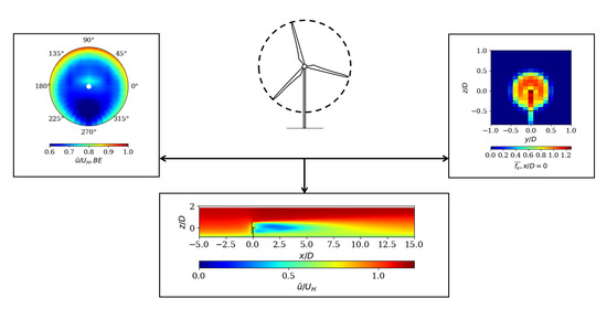
The general behavior of the flow around the turbine is characterized in Figure 2 and Figure 3. The effect of the turbine on the flow is clear. First, the turbine extracts energy from the flow, creating at the same time an induction region and a large wake region. The wake effect can be seen even at $x/D=15$ and is maximum around $x/D=2$. Secondly, the turbine modifies the turbulence of the flow, producing at the same time a strong increase of turbulence intensity at the turbine top tip level, and a reduction of turbulence intensity in the central and lower part of the wake, close to the turbine. The additional turbulence can be seen even at $x/D=15$ and the maximum appears around $x/D=4$. Overall, the general behavior of the flow is in agreements with previous studies [1,2,21,22].

3.1. Effect of the Force Projection Smoothing

In the following, the effect of the smoothing parameter is studied in detail by varying its value in the streamwise direction and the rotor plane directions independently. This leads to two independent smoothing parameters ${ϵ}_x$ and ${ϵ}_{yz}$ respectively (the turbine rotor is perpendicular to the x direction and aligned with $yz$ plane). Since Martinez et al. [5] showed that decreasing the smoothing parameter decreases the power, the reference simulation is defined with the smallest relevant smoothing parameter. In the x direction, the turbine is aligned exactly with the NS grid, which means that the BE grid points and the NS grid points are aligned in this direction. Therefore, the smallest possible smoothing parameter in this direction is ${ϵ}_x=0$. In the $yz$ directions, the BE grid points and the NS grid points are not aligned because the BE grid is polar and the NS grid is Cartesian. In these directions, the smallest relevant smoothing parameter is ${ϵ}_{yz}=R_{BE}$, where $R_{BE}$ is the radius of the corresponding BE, meaning that the turbine forces are projected from the BE grid to the NS grid with a smoothing parameter equal to the characteristic radius of the BE. It should be noted that this strategy is somehow different from the one used by Martinez and al. [5].

The effect of the x smoothing parameter is studied by taking ${ϵ}_x=0,1dx,2dx,3dx,$$4dx$. The vertical profiles of streamwise velocity deficit and added streamwise turbulence intensity downstream of the turbine are shown respectively in Figure 4 and Figure 5. It can be seen that the x smoothing parameter has almost no effect on the wake flow. The mean turbine aerodynamic coefficients and the mean rotor velocity are shown in

Table 1. Effect of the x-smoothing parameter on the turbine coefficients and rotor velocity. $C_T$ and $C_P$ are the mean thrust and power coefficients, respectively; $U_D$ is the mean rotor velocity; and $\delta \left(\right)$ is the relative difference with the default ${ϵ}_x=0$ case.

${\mathit{ϵ}}_{\mathit{x}}$	${\mathit{C}}_{\mathit{T}}$	$\mathit{\delta }\left({\mathit{C}}_{\mathit{T}}\right)\%$	${\mathit{C}}_{\mathit{P}}$	$\mathit{\delta }\left({\mathit{C}}_{\mathit{P}}\right)\%$	${\mathit{U}}_{\mathit{D}}$	$\mathit{\delta }\left({\mathit{U}}_{\mathit{D}}\right)$
exp	0.78		0.38
0	0.801		0.385		3.454
$1dx$	0.805	0.5	0.389	1.1	3.466	0.3
$2dx$	0.811	1.2	0.394	2.4	3.483	0.8
$3dx$	0.814	1.7	0.397	3.2	3.494	1.1
$4dx$	0.816	1.9	0.399	3.7	3.500	1.3

. It can be seen that the x smoothing parameter has a small effect on the rotor predictions. In particular, increasing the smoothing parameter increases the turbine coefficients and rotor velocity, with a larger increase for the power coefficient.

The effect of the $yz$ smoothing parameter is studied by taking ${ϵ}_{yz}=R_{BE},1dy,2dy,$$3dy,4dy$. The vertical profiles of streamwise velocity deficit and added streamwise turbulence intensity downstream of the turbine are shown respectively in Figure 6 and Figure 7. It can be seen that the $yz$ smoothing parameter has a clear effect on the wake flow. When the $yz$ smoothing parameter is increased, the velocity deficit is smoothed out in the near wake, with a smaller velocity deficit in the wake center and a larger velocity deficit away from the center. As a consequence, the shear at the wake edges is reduced. Consistently, the added streamwise turbulence intensity is globally reduced, and the peaks located around the wake edges are shifted towards the wake center. Interestingly, the differences decrease with the downstream distance, and the profiles are very similar at $x/D=8$. The mean turbine aerodynamic coefficients and mean rotor velocity are shown in

Table 2. Effect of the yz-smoothing parameter on the turbine coefficients and rotor velocity. $C_T$ and $C_P$ are the mean thrust and power coefficients, respectively; $U_D$ is the mean rotor velocity; and $\delta \left(\right)$ is the relative difference with the default ${ϵ}_{yz}=R_{BE}$ case.

${\mathit{ϵ}}_{\mathit{yz}}$	${\mathit{C}}_{\mathit{T}}$	$\mathit{\delta }\left({\mathit{C}}_{\mathit{T}}\right)\%$	${\mathit{C}}_{\mathit{P}}$	$\mathit{\delta }\left({\mathit{C}}_{\mathit{P}}\right)\%$	${\mathit{U}}_{\mathit{D}}$	$\mathit{\delta }\left({\mathit{U}}_{\mathit{D}}\right)$
exp	0.78		0.38
$R_{BE}$	0.801		0.385		3.454
$1dy$	0.822	2.7	0.404	4.8	3.515	1.7
$2dy$	0.870	8.6	0.445	15.5	3.685	6.7
$3dy$	0.911	13.7	0.477	23.9	3.871	12.1
$4dy$	0.941	17.5	0.502	30.5	4.035	16.8

. It can be seen that the $yz$ smoothing parameter has a very large effect on the rotor predictions. In particular, increasing the smoothing parameter increases the turbine coefficients and rotor velocity, with a larger increase for the power coefficient. Overall, it is clear that reducing the $yz$ smoothing improves the numerical results with respect to the experiment.

Overall, it is found that the effect of the smoothing parameter on the wake flow is much smaller than its effect on the rotor predictions, with the power being the most sensitive one. In addition, the effect of the smoothing parameter in the $yz$ directions is much stronger than the one in the x direction. These observations can be explained by looking carefully at the rotor predictions. For this, additional simulations were performed without including the effect of the nacelle and tower, to outline the raw effect of the ADM.

The non-dimensional axial forces, axial velocity and power distributions at the rotor when applying the reference smoothing, i.e., ${ϵ}_x=0,{ϵ}_{yz}=R_{BE}$, are shown in Figure 8. It can be seen that the axial force projected on the NS grid at the rotor plane is very close to the axial force computed on the BE grid. As a consequence, the axial velocity interpolated at the BE grid is consistent with the axial force computed at the BE grid. The axial force is found to be maximum in the mid-radius and upper part regions of the rotor and reduced in the large and small radius regions. The axial velocity at the rotor is found to be maximum in the upper part of the rotor. These elements are explained by the logarithmic profile of the incoming flow, the different contributions of the rotation to the relative velocity for different radius and the tip losses. The power distribution follows the axial force distribution with amplified differences in the distribution due to the stronger sensitivity of the power to the rotor velocity.

The non-dimensional axial forces, axial velocity, and power distributions at the rotor when applying a smoothing in the x direction of ${ϵ}_x=2dx$ are shown in Figure 9. In this case, the force is distributed (smoothed) on the neighboring grid points in the x direction. As a consequence, the axial force projected on the NS grid at the rotor plane is much reduced in comparison to the axial force computed on the BE grid (even though it is globally conserved). However, the distribution of the projected force on the NS grid is very similar to the one computed on the BE grid. In addition, the axial velocity distribution is consistent with the axial force computed at the BE and very close to the reference one. In this context, it can be concluded that the flow reacts to the additional smoothing similarly to the reference smoothing. This is due to the fact that the additional smoothing is performed in the streamwise direction, and therefore, the fluid feels a similar forcing on its trajectory. As a consequence, the axial force and power distributions computed at the BE are very close to the reference ones. This explains why the effect of the x smoothing on the flow and the turbine coefficients is small. However, since the force is not fully concentrated at the rotor plane, the force is slightly less effective at reducing the axial velocity at the rotor. This explains the small overestimation of the rotor velocity and the turbine coefficients. Also, the stronger sensitivity of the power to the rotor velocity with respect to the other rotor predictions explains the stronger sensitivity of the power on the x smoothing.

The non-dimensional axial forces, axial velocity, and power distributions at the rotor when applying a smoothing in the $yz$ directions of ${ϵ}_{yz}=2dy$ are shown in Figure 10. In this case, the force contribution of each BE is distributed (smoothed) on the neighboring NS grid points in the $yz$ directions. It can be seen that the axial force projected on the NS grid at the rotor plane follows a completely different distribution than the one computed on the BE grid (even though it is globally conserved). In particular, a larger part of the force is projected outside of the turbine rotor, the force is concentrated in the center of the rotor and the force is underestimated for mid-radius regions of the rotor. As a consequence, the axial velocity at the rotor is not consistent with the axial force computed at the BE, and the balance between the axial force and the axial velocity is broken. This means that the axial velocity is overestimated for locations with underestimated axial force (and vice versa). By comparing Figure 10 with Figure 8, it is found that the axial velocity is indeed largely overestimated in the mid-radius part of the rotor, corresponding to the underestimation of the projected axial force. By coupling effects, the axial force and power distribution computed at the BE are also different from the reference ones. These differences are explained by the differences in the axial velocity distributions. Overall, this explains the strong effect of the $yz$ smoothing on both the flow and the turbine coefficients. Also, the stronger sensitivity of the power to the rotor velocity with respect to to the other rotor predictions explains the stronger sensitivity of the power on the $yz$ smoothing.

One important aspect that has not been discussed here is the spurious numerical oscillations that can appear in the simulations due to sharp turbine forcing [5]. In the present case, when using some of the sharper smoothing configurations, some numerical oscillations have been noticed in the x and y directions, but not in the z direction (not shown here). In the code used in the present study, spectral methods are used in the x and y directions and 2nd order centered finite difference is used in the z direction. Since spectral methods tend to be more prone to develop oscillation than other methods, this result is not surprising. The fact that no spurious numerical oscillations were found on the z direction shows that these oscillations are a flow solver issue. Therefore, special care must be taken within the flow solver to control or avoid these numerical oscillations. In the present case, the observed results show that these oscillations are not harmful to the simulation results. However, more research should be conducted regarding this topic.

3.2. Effect of the Model Formulation

The effect of the model formulation is now studied in detail by comparing the results from the advanced ADM and the simple ADM presented in Section 2. Often, the implementations are slightly different between the models, which reduces the possible conclusions. For example, differences in the projection methods can lead to important differences in the results which are not directly related to the formulation of the model itself, as shown previously. Here, a strict equivalence of the implementations allow a rigorous comparison. In particular, the projection method is strictly equivalent, i.e., a Gaussian projection with ${ϵ}_x=0,{ϵ}_{yz}=R_{BE}$ is used in both cases. Also, both models consider the rotational effect of the turbine and compute the power from the tangential forces. The only difference between the two models is how the turbine forces are obtained on the BE grid. In the simple ADM, the turbine forces are reconstructed from the assumed turbine coefficients and a characteristic rotor velocity. As a consequence, the turbine effects are uniform over the rotor. In the advanced ADM, the turbine forces are computed using the blade element theory, i.e., using the local flow, the turbine geometry and the aerodynamic behavior of the turbine blades. As a consequence, a non-uniform distribution of the turbine forces over the rotor is applied.

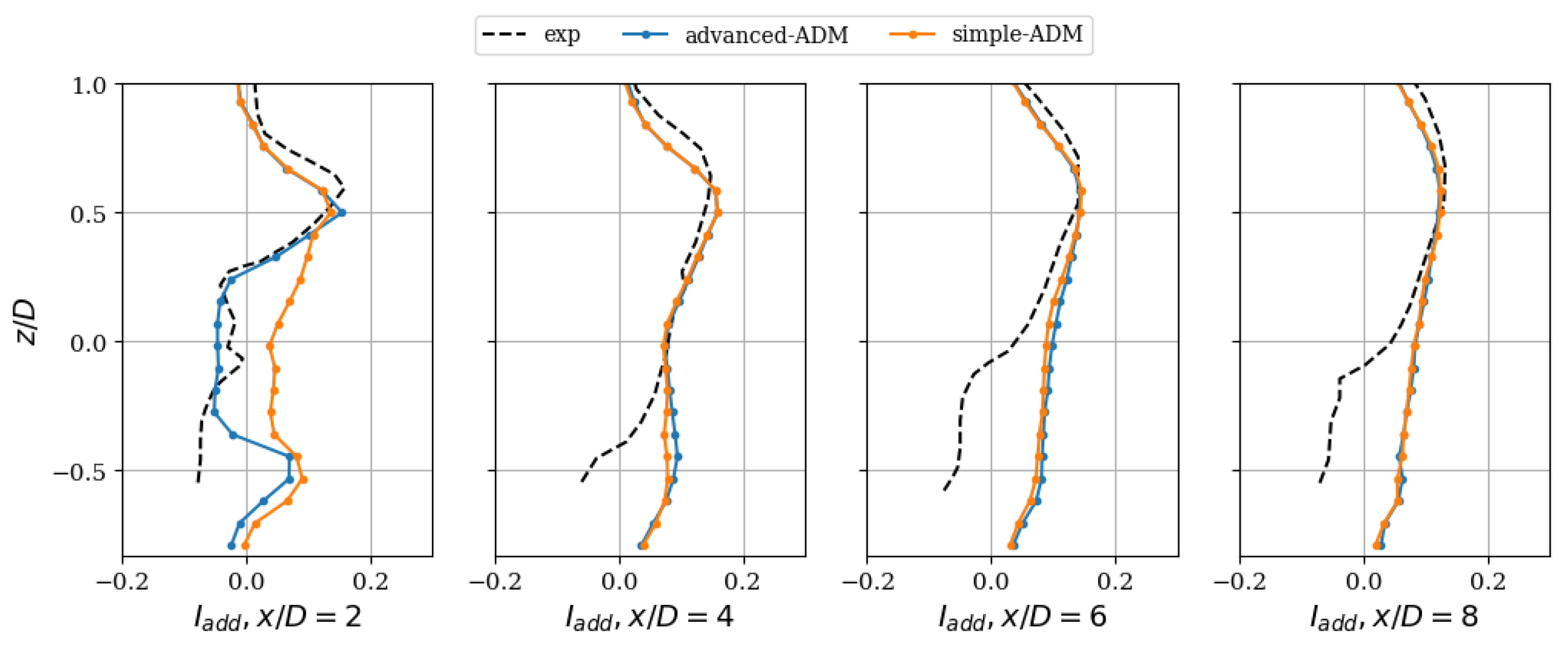
The vertical profiles of streamwise velocity deficit and added streamwise turbulence intensity downstream of the turbine are shown in Figure 11 and Figure 12, respectively. Some differences are evident for the profiles close to the turbine, for example at $x/D=2$ and 4, but the two models give very similar results after this. In the near wake, the simple model underestimates the streamwise velocity deficit and overestimates the added streamwise turbulence intensity with respect to the advanced model. The mean turbine aerodynamic coefficients and mean rotor velocity are shown in

Table 3. Effect of the ADM formulation on the turbine coefficients and rotor velocity. $C_T$ and $C_P$ are the mean thrust and power coefficients, respectively; $U_D$ is the mean rotor velocity; and $\delta \left(\right)$ is the relative difference with the default advanced ADM case.

	${\mathit{C}}_{\mathit{T}}$	$\mathit{\delta }\left({\mathit{C}}_{\mathit{T}}\right)\%$	${\mathit{C}}_{\mathit{P}}$	$\mathit{\delta }\left({\mathit{C}}_{\mathit{P}}\right)\%$	${\mathit{U}}_{\mathit{D}}$	$\mathit{\delta }\left({\mathit{U}}_{\mathit{D}}\right)$
exp	0.78		0.38
advanced	0.801		0.385		3.454
simple	0.790	−1.4	0.390	1.2	3.563	3.2

. The simple model correctly estimates the thrust and power coefficients, but overestimates the rotor velocity with respect to the advanced model. Overall, the advanced model improves the results in comparison to the experimental results.

The behavior of the simple model can be explained by its main assumptions (which are related together): (1) it computes the axial force from the rotor averaged velocity, and (2) it assumes a uniform axial force over the rotor. These assumptions do not allow for a local feedback between the axial force and the axial velocity. Therefore, when a non-homogeneity of the axial velocity exists, for example, because of the logarithmic profile of the inflow, the local force is underestimated for locations with a larger local velocity which will, in turn, increase the local velocity, and so on (and vice versa). This means that the distribution of the axial velocity across the rotor is not captured and, due to the non-linearities, this results here in an overestimation of the rotor velocity. Still, by construction, the simple model produces the correct thrust and power for this simple test case. This explains why the flow prediction is quite good once the local effects are reduced. However, for more complex cases where the local effects are important, e.g., in partial wake conditions, the simple model is expected to fail due to its inability to account for the local feedback between the axial velocity and axial force. In addition, the simple model relies on the power and turbine coefficients imposed, which therefore need to be accurate. Since those coefficients are only known for simple incoming flow conditions, it is expected that their use under complex flow conditions will further decrease the accuracy of the simple ADM model, e.g., due to topography or wake effects.

3.3. Effect of the Nacelle and Tower

The effect of the nacelle and tower is now studied in detail by comparing a simulation with the nacelle and tower included and one without these elements included. The vertical profiles of streamwise velocity deficit and added streamwise turbulence intensity downstream of the turbine are shown respectively in Figure 13 and Figure 14. Overall, the differences are small. The major differences are seen in the near wake in the hub and tower regions, where the velocity deficit is increased by the presence of the nacelle and tower. The mean turbine aerodynamic coefficients and mean rotor velocity are shown in

Table 4. Effect of the nacelle and tower on the turbine coefficients and rotor velocity. $C_T$ and $C_P$ are the mean thrust and power coefficients, respectively; $U_D$ is the mean rotor velocity; and $\delta \left(\right)$ is the relative difference of a given case with the case including the nacelle and tower.

	${\mathit{C}}_{\mathit{T}}$	$\mathit{\delta }\left({\mathit{C}}_{\mathit{T}}\right)\%$	${\mathit{C}}_{\mathit{P}}$	$\mathit{\delta }\left({\mathit{C}}_{\mathit{P}}\right)\%$	${\mathit{U}}_{\mathit{D}}$	$\mathit{\delta }\left({\mathit{U}}_{\mathit{D}}\right)$
exp	0.78		0.38
with nacelle and tower	0.801		0.385		3.454
without nacelle and tower	0.820	2.4	0.398	3.3	3.507	1.5

. It is found that the turbine coefficients and the rotor velocity are decreased when including the nacelle and tower, with a larger decrease for the power coefficient. Overall, it is clear that including the nacelle and tower improves the numerical results with respect to the experiment. However, it can be seen that the effect of the nacelle and tower is not fully captured. For example, the velocity deficit induced by the nacelle in the near wake is underestimated.

The effect of the nacelle and tower can be explained by looking carefully at the rotor predictions. The non-dimensional axial forces, axial velocity and, power distributions at the rotor are shown in Figure 15 for the simulation with the nacelle and tower included, and in Figure 8 for the simulation without these elements included. The additional forces from the nacelle and tower and their shadow effects are seen by comparing Figure 8 and Figure 15. When including the nacelle and tower, an additional drag force is included which reduces the axial velocity at the rotor plane around the corresponding locations. As a consequence, the axial force and power generated by the rotor are also reduced around these locations. The stronger sensitivity of the power to the rotor velocity with respect to the other rotor predictions explains the stronger sensitivity of the power on the nacelle and tower modelling.

3.4. Effect of the Grid Resolution

It is very important to study the sensitivity of the simulation results to the grid resolution. It is also very useful to know the coarsest resolution that can be used to obtain reasonably accurate results. This type of information can be used to optimize the use of computational resources, especially for large simulations. In this context, a grid resolution study is performed here by comparing four simulations with different grids. The different resolutions are presented in

Table 5. Definition of the grid resolutions used.

	$\mathit{D}/\mathit{dx}$	$\mathit{D}/\mathit{dy}$	$\mathit{D}/\mathit{dz}$
$G1$	3	6	9
$G2$	4	8	12
$G3$	5	10	15
$G4$	6	12	18

. Since ADMs are mostly preferred for coarse simulations, only relatively coarse grid resolutions are considered, i.e., in the order of 10 grid points along each direction across the rotor.

The vertical profiles of streamwise velocity deficit and added streamwise turbulence intensity downstream of the turbine are shown respectively in Figure 16 and Figure 17. The mean turbine aerodynamic coefficients and mean rotor velocity are shown in

Table 6. Effect of the grid resolution on the turbine coefficients and rotor velocity. $C_T$ and $C_P$ are the mean thrust and power coefficients, respectively; $U_D$ is the mean rotor velocity; and $\delta \left(\right)$ is the relative difference of a given case with its corresponding coarser case.

	${\mathit{C}}_{\mathit{T}}$	$\mathit{\delta }\left({\mathit{C}}_{\mathit{T}}\right)\%$	${\mathit{C}}_{\mathit{P}}$	$\mathit{\delta }\left({\mathit{C}}_{\mathit{P}}\right)\%$	${\mathit{U}}_{\mathit{D}}$	$\mathit{\delta }\left({\mathit{U}}_{\mathit{D}}\right)$
exp	0.78		0.38
$G1$	0.827		0.409		3.533
$G2$	0.801	−3.2	0.385	−5.6	3.454	−2.2
$G3$	0.794	−0.8	0.379	−1.5	3.450	−0.1
$G4$	0.793	−0.1	0.378	−0.3	3.454	0.1

. The convergence of the results is clear, with the results showing little resolution dependence when more than 8 and 12 grid points are used along the spanwise and vertical directions respectively. Overall, the agreement with the experimental data is quite good. In particular, the difference between the fine simulation and the experimental data for the thrust and power is in the order of $1\%$ which is well within the experimental uncertainty [21,22]. The major differences in the wake flow prediction are the underestimation of the velocity deficit near the hub in the near wake and the overestimation of the added turbulence in the lower part of the rotor in the far wake. Both of them can be related to the effect of the nacelle and tower which is not captured accurately. Indeed, with the coarse grid resolutions used, i.e., with grid resolutions in the order of 10 grid points across the rotor, the nacelle and tower elements are not well resolved. A proper resolution of these elements would require a much finer resolution that would be unpractical for many applications.

4. Summary

A new evaluation of ADMs with a special focus on the implementation details, and the power prediction has been performed. In contrast with previous similar studies, this evaluation is based on a case with a realistic boundary-layer inflow, and for which accurate data for the flow, thrust, power, turbine geometry and aerodynamic behavior of the turbine blades are available.

First, the effect of the force projection smoothing parameter has been studied in detail. Overall, it is found that the smoothing parameter has a strong impact on the rotor predictions and a moderate impact on the wake flow. Therefore, for studies focusing on the wake flow, the smoothing parameter is not as critical as for studies focusing on rotor predictions. In addition, it is found that increasing the smoothing parameter increases the rotor predictions, leading to an overestimation of these, and with the strongest increase/overestimation for the power prediction. By studying the effect of the smoothing parameter in the streamwise direction and the rotor plane separately, it is found that the smoothing in the streamwise direction has only a small effect on the results while the smoothing in the rotor plane has a strong effect. This means that non-isotropic projections and grids should be used to optimize the computational setup. Also, it is found that the effect of the smoothing parameter is directly related to the consistency between the axial force computed on the BE grid and the axial force projected on the NS grid. When an inconsistency exists, the feedback between the axial force and axial velocity at the rotor plane is broken. This leads to an overestimation of the axial velocity at the rotor plane which in turn leads itself to an overestimation of the thrust and power predictions. As a consequence, when designing ADMs, a projection method that conserves the force distribution on the rotor should be used if the rotor predictions are of interest. In contradiction with Martinez et al. [5], it is found that numerical oscillations originating from very sharp forces are not harmful to the results. Several factors could explain this difference, including the type of inflows, the numerical methods, and the smoothing definitions. Also, more research should be conducted regarding this topic.

Secondly, the effect of the model formulation has been studied in detail. In the literature, many different implementations of ADMs have been used. Here, it is proposed to divide these models into two categories: (1) simple ADMs, and (2) advanced ADMs. These two categories of models are defined based on how the models compute the turbine forces. In simple models, the turbine forces are reconstructed from assumed turbine coefficients and a characteristic rotor velocity. As a consequence, the effects of the turbine forces applied are uniform over the rotor. In advanced models, the turbine forces are computed using blade element theory, i.e., using the local flow, the turbine geometry and the aerodynamic behavior of the turbine blades. As a consequence, the turbine forces applied are non-uniform over the rotor. Here, a simple model is compared to the reference model (advanced model), and a fair comparison is ensured by a strict consistency between the implementations. Overall, both models reproduce quite well the far wake flow and provide accurate thrust and power predictions. However, it is found that the advanced model performs better than the simple model in the near wake. In particular, it is found that the simple model underestimate the velocity deficit and overestimate the added turbulence in the near wake in comparison to the advanced model and the experimental results. In addition, the simple model shows an overestimation of the rotor velocity in comparison to the advanced model although the thrust and power predictions are very similar. These elements are explained by the assumption of uniform axial force distribution over the rotor used in simple models. The assumption indeed does not allow for the local feedback between the axial force and the axial velocity, meaning that the local balance between the axial force and the axial velocity is broken. In addition, the dependence of these models on the assumed turbine aerodynamic coefficients can further decrease their accuracy under complex flow conditions, where the turbine aerodynamic coefficients are not known accurately.

Thirdly, the effect of the nacelle and tower has been studied in detail by comparing a simulation with the nacelle and tower included and a simulation without these elements included. It is found that, when including the nacelle and tower, the velocity deficit in the near wake is increased and the rotor predictions are reduced, due to the shadow effect of the nacelle and tower. Overall, the consideration of the nacelle and tower improves the near wake predictions and the rotor predictions. However, it is important to note that the flow around these elements cannot be captured in detail due to the coarse resolutions typically used for this type of simulation.

Finally, a grid convergence study has been performed. It is found that the simulations show a clear convergence, with the results showing little resolution dependence when around 10 grid points are used along each direction across the rotor. The simulations show very good agreement with available experimental data. In particular, the streamwise velocity and streamwise turbulence are well captured in the wake, and the turbine thrust and power are predicted accurately (within the experimental errors). Still, some small differences can be seen for the velocity deficit in the near wake around the nacelle, and for the added turbulence close to the ground. These differences are most likely due to the failure of the simulations to accurately capture the effect of the nacelle and tower, as discussed above. Interestingly, it is found here that in the convergence process, the power prediction is reduced when the grid is refined. This is in contradiction with the findings from Martinez et al [5]. Also, the results converge with a grid size that is much coarser with respect to the smoothing parameter than the guidelines proposed by Martinez et al. [5]. Again, several factors could explain these differences, as discussed above.

Overall, the comparison with the experimental data shows that an accurate prediction of the flow, thrust and power is possible with a very reasonable computational cost. In addition, the results of this work give general guidelines for the use of ADMs in the context of LES of wind turbine flows. They also contribute to further optimize and validate the present numerical framework. In particular, this LES framework will be used to study wind turbine wake flows in more complex conditions.