1. Introduction
In this paper, a prediction of solar irradiance was proposed based on a sky image that includes the sky, clouds and their movement, and sun coverage. The motivation for this research was to obtain a solar-based virtual power plant. In such a plant, the maximum production limit curve for a future period could be obtained from the long-term hourly irradiance forecast of the hydrometeorological institute. The production limit curve is essential for the power system dispatcher to ensure the stability of the power system. The irradiance forecast represents the average hourly irradiance. In order to achieve the planned average power generation, it is necessary to use energy storage to compensate for the deviation of the current irradiance from the average. Optimal use of energy storage devices with different efficiency, capacity, and response times can be achieved if the more accurate irradiance prediction for the time interval of the next hour is available.
The 1-h horizon forecast elaborated in this paper is based on cloud motion prediction and a wide-angle ground camera that takes a picture of the sky every 5 s. The direction of cloud movement is calculated from the movement of their centroids and the detected cloud edges within 1 min (after taking 12 consecutive images of the sky). Based on the visible clouds in the sky and their movement, the prediction of the clouds, the position of the sun, and the prediction of the solar irradiance are performed. The described method has proven to be simple since the shape of the clouds and the sun is approximated by a rectangular shape based on only four points, which does not depend on sophisticated algorithms and does not require the training of neural network models based on large data sets. The strength and novelty of this research are in its simplicity (it approximates the shape of the clouds with rectangles) that makes it practical and performant (the movement simulation of clouds and sun is based on moving only four points that define the rectangle shape). Additionally, it can be used in a virtual plant environment based on only one commercial camera and with the prediction of sun coverage level with clouds during the following hour period. Therefore, there is no need to use satellite images of the sky and gather data for training models based on machine learning.
Prediction of solar radiation has been the subject of many studies in recent years. Some studies have introduced artificial neural networks or deep learning with extensive data sets. Examples of solar radiation prediction based on machine learning [
1,
2,
3,
4,
5,
6] showed that solar radiation prediction could be affected by different input parameters for artificial neural networks and multilayer perceptrons. The other machine learning method based on publicly available weather reports showed the approach for a prediction horizon of 24 h [
7]. One of the methods described a prediction accuracy of 2 days in advance based on a dataset covering a period of 8 months [
8]. These methods allow the development of a system that operates autonomously but depends on collected data and the training of a model that must be retrained as parameters change over time. Moreover, if the prediction period is too long, the approach is not suitable for microgrid systems that support different types of energy storage [
9,
10,
11] based on dynamic adaptation and parameters of the system based on capacity, current load, and speed of energy storage. Compared to the method described in this paper, machine learning-based systems require a large set of historical data and time to train the models to make the prediction. Furthermore, the need to retrain the model after collecting new datasets after deploying the production system to improve it does not exist. The model described in this paper does not depend on existing historical data.
Other methods used cloud motion prediction based on satellite images and motion vectors to predict output power, but only 30 min in advance, which may be a limitation, especially when some power storage devices in the microgrid system need more time to change their operating mode from charging to discharging [
12]. A similar method has been used with several fisheye cameras but could predict up to 15 to 30 min of updates per minute [
13], but our method manages to predict solar coverage up to 1 h.
The development of cloud detection algorithms based on sky images has also received many variants. One of the approaches analyzed the way of reducing sunlight interference in ground-based sky images [
14]. It has been shown that HSV color space gives the best results, so the same approach is used in this work to accurately detect the cloud edges, cloud centroid, and cloud motion. Optimal HSV thresholds for best results in cloud edge detection can be determined by an artificial neural network-based system described in our previous work [
15] since the sky image often contains different parameters (number of clouds, cloud sizes, and histogram values) and colors that may require different settings for image processing. Other variants of cloud detection on sky/cloud images captured by ground-based cameras are based on cloud segmentation [
16], which is learning-based and not suitable for rapidly changing weather conditions. Some research involved artificial neural networks that depend on the datasets for a given area [
17,
18]. These approaches are only suitable for specific areas and often cannot be applied to all locations.
An Internet of Things-based solution for intra-minute cloud passing forecasting that uses the cloud’s center of gravity can also be used to control the reduction of the output power of photovoltaic systems [
19]. However, the proposed solution is focused on the short-term prediction of the moment when the clouds start to cover the sun, which may be too short to effectively control different types of energy storage devices in a microgrid system.
Satellite images, together with a support vector machine learning scheme, can also be used for solar power prediction as well [
20], but the approach is not suitable for solar systems that are located at a specific geographical location and depends on the position of the clouds and the sun.
Cloud motion estimation based on a block matching algorithm performs the motion of a pixel block over a region and searches for two blocks in two consecutive images that have the highest degree of similarity [
21], which proves that using sky images is a reliable method for cloud motion prediction. The only challenge with this approach is the longer processing time, making it challenging to use under real-time conditions.
This work is based on the assumption that the long-term irradiance forecast with hourly resolution from the hydrometeorological institute is accurate enough to be used as an upper bound reference for scheduling energy production for the power system dispatcher. To obtain the declared constant hourly interval production equal to the declared possible production based on the average hourly estimates, it is necessary to use an energy storage system. If the energy storage system consists of different storages with different capacities, efficiency, and response speed, the efficient use of these storages is possible if an accurate forecast of irradiation is available with a maximum of 1 min time sample in a 1-h forecast window. For this purpose, it is necessary to obtain a curve of the percentage of the uncovered sun with clouds for 1 h in the future. Normalizing the mean of this curve to the value predicted by the hydrometeorological institute should give the accurate curve of irradiance for that time. The curve of predicted irradiance, corrected with coefficients characteristic of the production facility, could serve as a basis for online optimization of the use of the power system. The solar coverage prediction is based on wide-angle camera images of the sky.
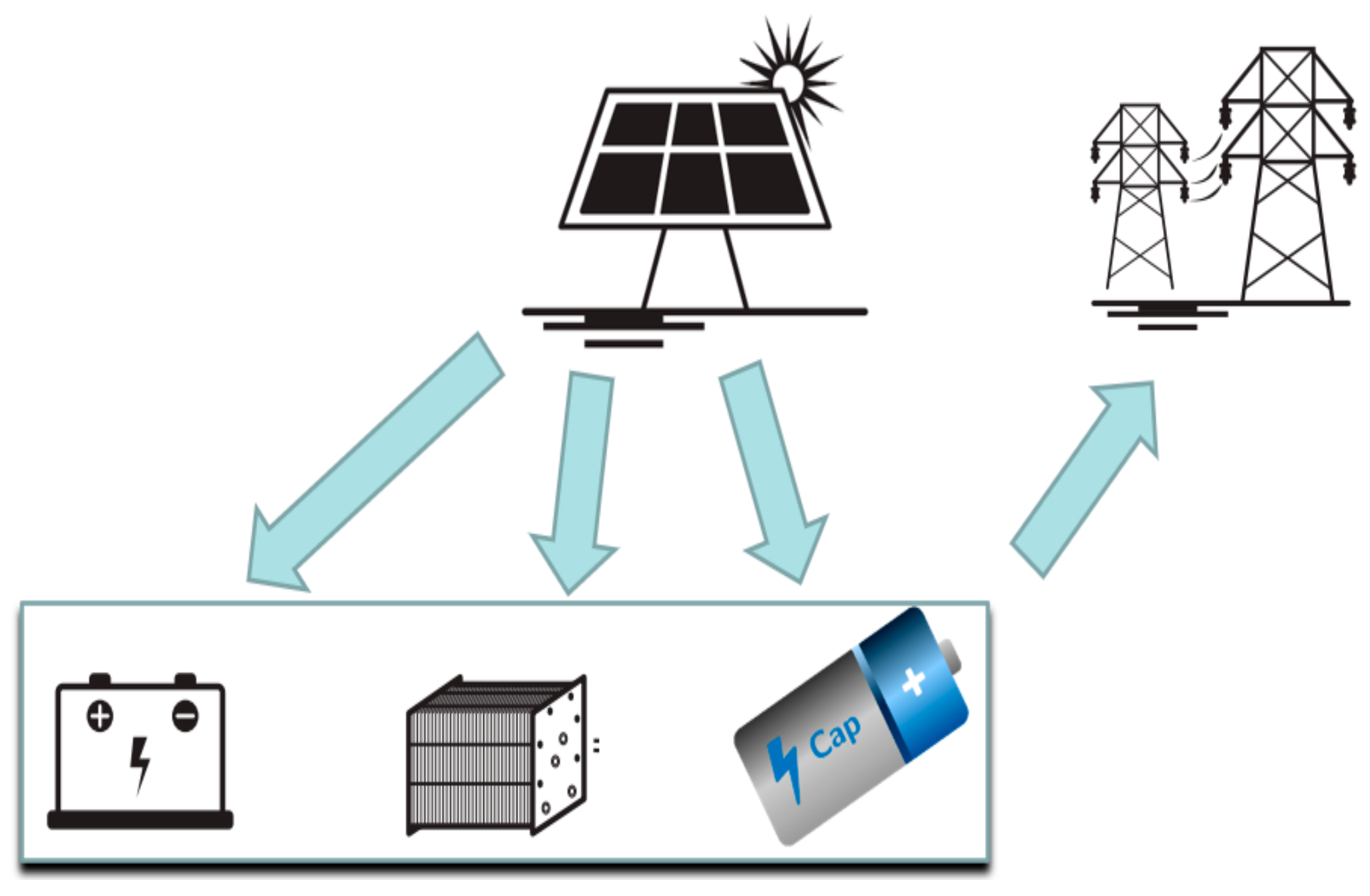
The possible utilization of this prediction model and the generated curve of predicted solar irradiance is in a virtual plant that consists of different storages and is based on integration with solar photovoltaic cells. Storages can be based on a battery [
22], hydrogen cell [
23], and supercapacitor [
24], each with different characteristics related to capacity, efficiency, and response speed. With the generated curve of predicted solar irradiance in the next hour, the amount of energy generated can be predicted. Depending on the energy storage condition in terms of their charge, efficiency, and response speed, it can be determined which storage should be used to store generated energy. If the sun is visible in the next period, the solar energy will be generated and stored in one of the storages, or if the sun is not visible, then the stored energy needs to be consumed. Among different storages, optimizing energy flows ensures the use maximization of stored energy [
25].
Section 2 describes the master control algorithm of sun un-coverage forecast in the hybrid storage system. It contains a flow diagram of the algorithm with a description of the sequence of steps.
The algorithm for detecting the sun and clouds is obtained in
Section 3, where camera calibration is described and contour and centroid detection of both the sun and clouds.
The list of clouds that are candidates for sun coverage according to their current position and velocity vector is obtained in
Section 4. The irradiance curve is obtained in the same section using subsequent calculation of cloud position and sun coverage with a determined time sample.
The results of sun un-coverage percentage prediction and real-time un-coverage percentage comparison are presented in
Section 5, while the concluding considerations and list of references are given in
Section 6, respectively.
3. Clouds and Sun Detection Algorithm
Ground-based sky images were captured from the site in Zagreb, Croatia, using the GoPro Fusion wide-angle camera with authors as photographers during the experiment. The sky images for the experiment were captured with a sampling time of 5 s, starting on 12 July 2020 at 10:28:50 h until 15 July 2020 08:25:20 h.
Figure 1 shows few examples of captured images that are cloud-free or contain different types of clouds. The east is on the left side of the images, the west on the right side, the north at the bottom of the image, and the south at the top of the image.
The image in
Figure 3a shows an example of an image with a clear sky without clouds (it was taken on 13 July 2020 at 08:09:09),
Figure 3b an image with many cumulus clouds (it was taken on 13. July 2020 at 13:26:20),
Figure 3c an image with cirrus clouds (it was taken on July 14 at 09:09:15), and
Figure 3d an image taken at the end of the day when the sun was setting over the horizon (it was taken on July 14 at 18:45:32).
From the images in
Figure 3, it can be seen that the wide-angle camera used distorts the image quite a bit. In order to obtain a linear motion of the cloud according to its velocity vector, it is necessary to undistort the image.
3.1. Camera Calibration
In order to correct the distorted image of the GoPro Fusion camera and define the parameters of the undistortion algorithm, a camera calibration was performed. For this purpose, the image of the checkerboard 100 cm × 90 cm with the size of the squares 2 cm × 2 cm is used.
Omni directional Camera Calibration Toolbox for Matlab [
26,
27,
28] is used for image undistortion. It allows the user to calibrate any omnidirectional camera in two steps: collecting multiple images of a checkerboard shown in different positions and orientations and extracting the vertices. After calibration, it provides functionalities to express the relationship between a given pixel point and its projection on the unit sphere. The calibration procedure starts with the selection of images with checkerboard patterns and continues with the detection of the checkerboard points using the method “detectCheckerboardPoints”. The image size is determined based on the first image read. In our case, the image resolution was 3104 × 3000 pixels. In the next step, the square size of the checkerboard is determined and the world coordinates of the corners of the squares are generated using the method “generateCheckerboardPoints”. After that, the calibration is performed based on the fisheye parameters using the method “estimateFisheyeParameters”. The last phase is the undistortion of the image using the method “undistortFisheyeImage”.
Figure 4a shows the distorted checkerboard used for camera calibration, and
Figure 4b shows the undistorted version after the described procedure has been performed.
Figure 4d,e show the distorted and undistorted version of the image with the clouds and the sun located in the center of the image,
Figure 4f,g show the distorted and undistorted version of the image with the sun located on the left side of the image (near the east).
Figure 4c shows the Matlab generated visualization of the extrinsic parameters after running the “show Extrinsics” function. It shows the rendered 3-D visualization of the extrinsic parameters by viewing the calibration patterns with respect to the camera. It plots the locations of the calibration pattern in the camera’s coordinate system that were taken during the calibration phase. Each enumerated location represents a different angle, position, and distance of the checkerboard from the camera taken during the calibration time. The location of the camera is shown in dark blue, and the positions of the board with checkerboards are shown in other colors in
Figure 4c. Different colors are used to make the image distinguishable more easily. Only those images with checkerboards are considered valid that contain a complete visible board [
29].
The obtained undistorted images allow the calculation of the cloud position and velocity.
After undistorted images of the sky were obtained, the next step is to recognize the contour and center of gravity of the sun, described in the following section.
3.2. Recognition of the Contours and the Center of Gravity of the Sun
The flowchart of the image processing algorithm mentioned in the previous section is shown in
Figure 5.
The first phase of the algorithm used is to undistort the image and then detect the contour of the sun, the centroid of the sun contour, and then the contours of all the clouds in the image and their corresponding centroids. To improve the detection results, only significant areas of the sun and cloud contours are considered. For the sun contour, the range of 5000 pixels is used as the threshold for detecting the sun. When a cloud starts to partially cover the sun, the area of the sun shrinks, and when the area is below the aforementioned 5000 pixels, the sun is considered to be covered by clouds. The threshold is based on the camera resolution (3104 × 3000 pixels) and the visible area of the sun in the clear or uncovered sky, as shown in
Figure 6c. It is determined by the calculated area of the sun during the period of taking pictures of the sky and using a minimum value of the area when the sun is visible and not covered by clouds.
As with the sun area threshold, only clouds with the significant area are considered since those with too small of an area do not significantly block the sun. The threshold for cloud area is set to 3000 pixels: clouds with an area less than 3000 pixels are simply ignored and not stored in the ArrayList structure in the Java programming language with other clouds that may significantly cover the sun. The cloud area threshold is based on the sun area threshold: if the calculated cloud area is 60% of the calculated sun area, it is considered a significant coverage level.
The first step is to detect the sun in the sky by performing morphological operations of erosion. To detect the sun, the following image processing operations must be performed first (as described in our previous work [
30]): converting the image from RGB (Red, Green, and Blue) to HSV (Hue, Saturation, and Value) color model, setting the size for structured elements for erosion, finding contours on the image that represent the sun, and finding the sun’s centroid.
Morphological operations on a binary image create a new binary image in which the pixels have a non-zero value only if the test succeeds at the location in the image. A structuring element is a binary image represented by a matrix of pixels that have values of zero or one. The dimensions of the matrix indicate the size of the structuring element. The erosion of a binary image is described with the following equation:
where
represents the new binary image after erosion operation,
is the initial binary image that was transformed, and
represents the structuring element.
In the resulting image, there are ones at the coordinates (x, y) of the origin of a structuring element where it matches the input image , (x, y) = 1 if the structuring element matches and zero otherwise. In the case of sun detection, erosion removes clouds from a binary image, and in the case of cloud detection, it removes very small clouds and reduces the size of clouds to emphasize the boundaries between clouds. The dilation operation has the opposite effect on erosion: it adds a layer of pixels to both the inner and outer boundaries of the contours.
The conversion from the RGB color model to the HSV color model can be done with the JavaCV library (based on the OpenCV library written in C++) using the method “cvtColor” from the class “Imgproc”. Since the images containing the sun consist of glittering segments, the minimum and maximum values for the H and S components can be set to 0 (this represents the filter that suppresses the H and S components), but the V component is set from a minimum value of 240 to a maximum value of 255.
Figure 6a shows the initial RGB image and the resulting HSV image afterward in
Figure 6b.
The structuring element used in erosion was set at the size of 50
× 50 pixels. The size was determined based on the image resolution (3104
× 3000 pixels) and the criteria for detecting the most glittering element on the image, namely the sun.
Figure 5 shows the steps that were performed to detect the sun:
Figure 6a shows the original image,
Figure 6b shows the sky image converted to HSV format using the minimum HSV components (0, 0, 240) and the maximum values (0, 0, 255),
Figure 6c shows the image after the erosion process (the white part represents the detected sun), and
Figure 6d shows the image with the detected contour, the centroid point as well as the rectangular approximation to the shape of the sun contour (drawn in red). The H and S components of the HSV minimum and maximum values are set to zero to ignore the color component portion of the model (with H component) and the amount of gray (with S component). The value for the V component is the only component used because it describes the brightness of the color. The minimum and maximum values, set to 240 and 255, respectively, give the best results for detecting the most glittering element in the sky, namely the sun.
After detecting the sun and applying the erosion operation, the only contour detected on the image was the contour of the sun. Using the “findContours” method available in the “Imgproc” class of JavaCV, the sun contour is accurately detected and drawn using the “drawContours” method in
Figure 6d. In addition to the sun contour, a minimum-area bounding rectangle enclosing the contour points is found using the “minAreaRect” method from the “Imgproc” class in the same figure.
As clouds are moving over the horizon, the sun is moving as well, although much slower than the clouds. To detect the sun movement, the centroid of the sun needs to be detected. Since the images were taken every 5 s, the sun movements are often very small, but the sun travels over the whole sky during the day. The sun’s centroids are calculated as the arithmetic mean of all the contour points as shown in Equation (2):
where
c is the centroid of the sun,
n is the number of points in the contour, and
are the coordinates of the points in the contour.
To find the center of gravity of the sun in JavaCV, moments must be used. A moment is a certain weighted average of the intensities of the image pixels that can be used to find some specific properties of an image, such as the centroid. In the case of a raster image, the spatial moments are calculated as [
31] shown in Equation (3). The central moments are calculated using Equation (4), where
is the centroid calculated using Equations (5) and (6).
where
represents the spatial moment,
is the array of 2D points of the image,
and
are coordinates of points,
is the central moments, and
represents the center of mass.
Figure 6d shows the detected centroid of the sun (the red circle inside of the sun contour).
3.3. Detection of the Contours and the Centroid of the Sun
After successfully locating the sun and detecting the centroid with contour, the next step was to detect clouds on the image. The process of cloud edge detection consists of converting the color model, applying the morphological operations erosion and dilation, and shape approximation with the bounding rectangle with minimum area. The images generated during the process are shown in
Figure 7.
The minimum and maximum values for the HSV components were set to (0, 0, 0) and (70, 70, 255) to obtain the best results. Compared to the parameters used for sun detection, where only the most glittering element on the image was in focus, cloud detection also focused on other colors, such as different shades of gray. The H-component is the color component of the model, and with values between 0 and 70, the dominant color is red (
Figure 7b). The S component describes the amount of gray in a given color, and reducing this component results in a more gray color, which is a very common color of clouds. The V component is not filtered, covers the entire range from 0 to 255, and in conjunction with saturation, describes the brightness of the color to cover all shades of gray. The original image is shown in
Figure 7a, and the image transformed to the HSV color model is shown in
Figure 7b.
The size of the structuring element for the morphological operation of erosion was set to the size of 20 × 20 pixels, and it was determined using the image resolution (3104 × 3000 pixels) and the criteria for the removal of very small clouds (with the calculated area below 3000 pixels). The resulting image after transformation is shown in
Figure 7c. In order to obtain the best results in cloud edge detection, after applying the erosion operation, a dilation operation was performed based on structural elements with the size of 30 × 30 pixels. The size was determined based on the image resolution and the criterion of filling small holes in clouds that appeared after applying the erosion operation. In the case of detection of the sun, the application of the dilation operation was not necessary since it is the most glittering element on the image, only erosion. The results of the transformation can be seen in
Figure 7d.
After the sun and cloud contours have been detected and saved, altogether with their centroid points, the next phase of our algorithm is to determine the sun coverage level based on cloud’s and the sun’s speed vectors, described in the following section.
5. Results
After the cloud motion simulation was performed, the degree of sun coverage was calculated for each time period in the future as long as the tracked clouds were present in the undistorted image. The comparison of the actual and predicted sun coverage level is shown in
Figure 12 and
Figure 13. The data shown covers the period on 13 July 2020. from 13:45 to 14:40 and from 12:00 to 12:45.
Figure 12,
Figure 13,
Figure 14,
Figure 15,
Figure 16,
Figure 17,
Figure 18 and
Figure 19 show the situation in the sky where several clouds were moving towards the sun and corresponding error levels. The red curve, which represents the real-time sun un-coverage level on images that compare the real-time and predicted sun-uncoverage level, shows that the visible area of the sun changes significantly in a nonlinear manner as the clouds begin to cover or uncover the sun. This effect is caused by the transparent nature of the clouds, which prevents the sun from being completely covered at the beginning of the cloud coverage process, while the rectangular shape approximation does not take this effect into account. The real-time sun un-coverage level is based on the detected area of the sun when it is covered with clouds compared to the area of the sun when there are no clouds. The corresponding error levels are marked with red curve, and standard error value with blue curve.
The predicted level of coverage, based on the rectangular shape approximation obtained by the described algorithm, covers and uncovers the sun region in a linear manner, as shown by the blue curve in
Figure 12,
Figure 14,
Figure 16 and
Figure 18, with corresponding prediction error levels shown on
Figure 13,
Figure 15,
Figure 17 and
Figure 19, respectively. The blue curve in
Figure 12,
Figure 14,
Figure 16 and
Figure 18 represents a prediction. It was performed at the beginning of the period of 1 h: in
Figure 12 at 13:47, in
Figure 14 at 12:03, in
Figure 16 at 10:34, and in
Figure 18 at 16:38. After the algorithm analyzed the position change of the clouds and the sun during the last minute (12 images were used, each image was taken every 5 s), the prediction was performed for the next hour. The prediction (blue curve) was compared to the real-time un-coverage level (red curve) that was measured after the prediction was performed to calculate the error level. The real-time curves and the predictions match in the critical areas where the sun is fully covered or fully exposed.
The obtained curve can be used to predict the amount of direct solar irradiance calculated according to the following equation:
where
represents estimated irradiance in
,
is the estimated sun un-coverage level measured in percentages (represented by the blue curves in
Figure 12,
Figure 14,
Figure 16 and
Figure 18),
represents predicted average irradiance estimation of direct solar irradiance based on the 1-h time period provided by the meteorological and hydrological service measured in
, and
represents the predicted average value of predicted sun un-coverage level (measured in percentage from 0 to 100%).
The standard error level shown in
Figure 13,
Figure 15,
Figure 17 and
Figure 19 shows that it is in range of 10–20%. The results show that it is the highest in periods when clouds start and with sun coverage, especially if the clouds are transparent and the sunlight can break through them.
In cases when the sun is positioned near to the horizon, with an orientation where the clouds come from to the horizon (for example, the east side is on the left part of the taken sky images) during the morning (as shown in
Figure 16), the prediction possibilities are limited. This is because of the short distance between the sun and the clouds. However, total irradiance is usually lower during the morning, so the absolute error related to the energy amount is lower as well. Therefore, optimal prediction is obtained when the sun is positioned further away from the cloud positions (for example, in the middle of the day, during noon).
The meteorological and hydrological service provides forecast values for direct solar irradiance for a selected area for the next 64 h and provides an average value of solar irradiance per hour. Based on the prediction of the sun coverage with clouds, the average value of direct solar irradiance can be estimated, as shown in
Figure 20,
Figure 21,
Figure 22 and
Figure 23.
Since the minimum-area bounding rectangle shape approximations were used for the cloud and solar contours, the algorithm proved to be very simple and requires an average time for estimating the sun coverage between 5 and 6 s. The simulations were run on a personal computer with the Intel Core i7-8750 processor (2.20 GHz) with 24 GB of RAM (1 GB was used for the integrated development environment for Java) with an SSD disk drive with sequential reading up to 2800 MB/s.
6. Conclusions
The results show that the cloud positions can be determined with respect to the position of the sun if the contour shapes are approximated with a minimum-area bounding rectangle. The shape approximation has no significant effect on the estimation of the beginning and end of the cloud shadow over the sun. The simplicity and speed of the described algorithm make our approach for estimating direct solar irradiance suitable for use in solar-based virtual power plants. Error measured between the predicted and real-time un-coverage can be used as a security limit when designing the storage systems. The predicted amount of generated energy can be decreased to avoid wrong optimistic predictions that can affect the stability of a virtual power plant. The error cannot be determined online, but based on experience gained through the measurements and different periods during the day.
The presented results show that a short-term prediction based on a ground camera and the use of the estimated degree of sun coverage in combination with the hourly average solar irradiance forecast provided by the meteorological and hydrological service can be used to predict the amount of direct solar irradiance. The short-term prediction is performed as soon as a cloud appears on the sky image captured by the camera so that after a fixed period of time has elapsed (1 min or 12 images captured every 5 s), the estimation process can be automatically started. The only limitation is based on solar visibility. The estimation process can begin when the initial position of the sun has been captured.
Future work will include comparison with measurement data collected with a pyranometer instrument and will include all periods of the year, including fall, winter, spring, and summer, to cover all possible types of clouds. The options, such as adapting the system to different seasons and cloud types, can be upgraded with a machine learning component that replaces manual human work and improves the autonomy of the system. In addition, the direct solar irradiation curve obtained by prediction could be used to optimize the energy flows in a microgrid with a photovoltaic system, including energy storage devices.
The article shows one of the methods for short-term solar irradiance prediction based on cloud motion prediction. The study involved the installation of a manual camera placed on the roof of the residential building and offline processing of the images. The results prove that a microgrid system based on different energy storage devices with different parameters (such as the capacity, the delay between the change of mode from charging to discharging, etc.) is suitable for short-term prediction, focusing on the period from half an hour to 1 h.


