
MPC Based Coordinated Active and Reactive Power Control Strategy of DFIG Wind Farm with Distributed ESSs

Abstract
:1. Introduction
2. Coordinated Active and Reactive Power Control Structure
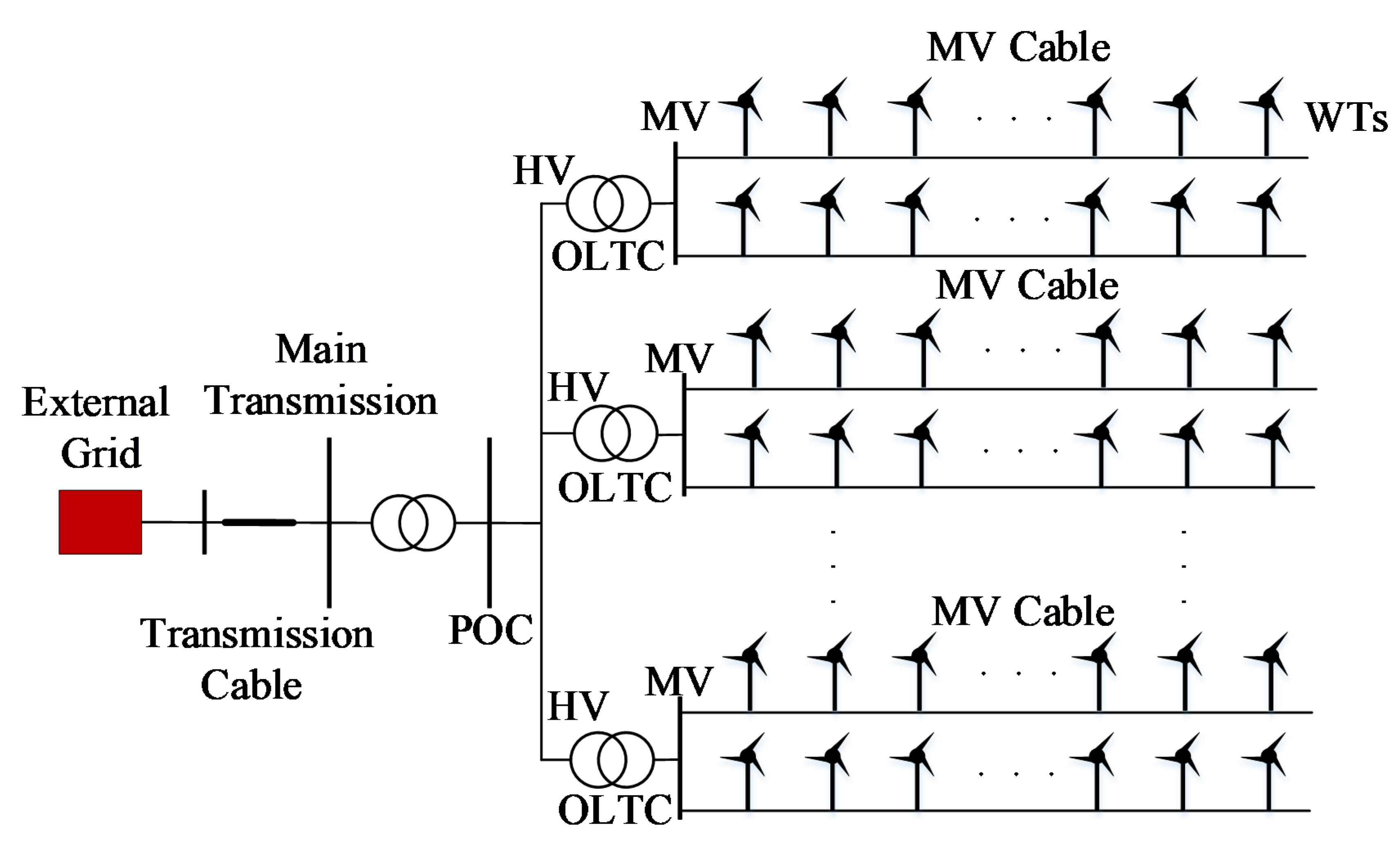
2.1. Configuration of DFIG Wind Farm
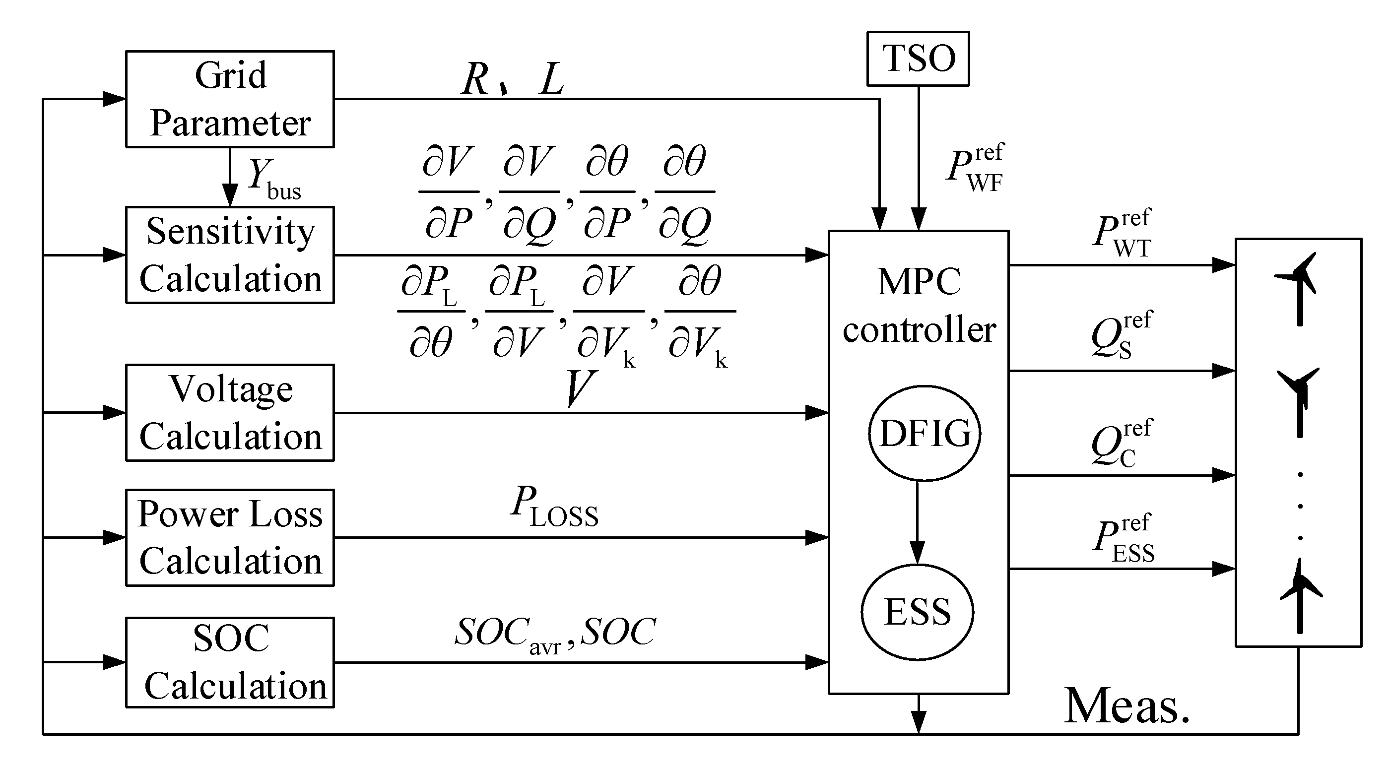
2.2. Concept of Coordinated Power Control Scheme
3. WF Model
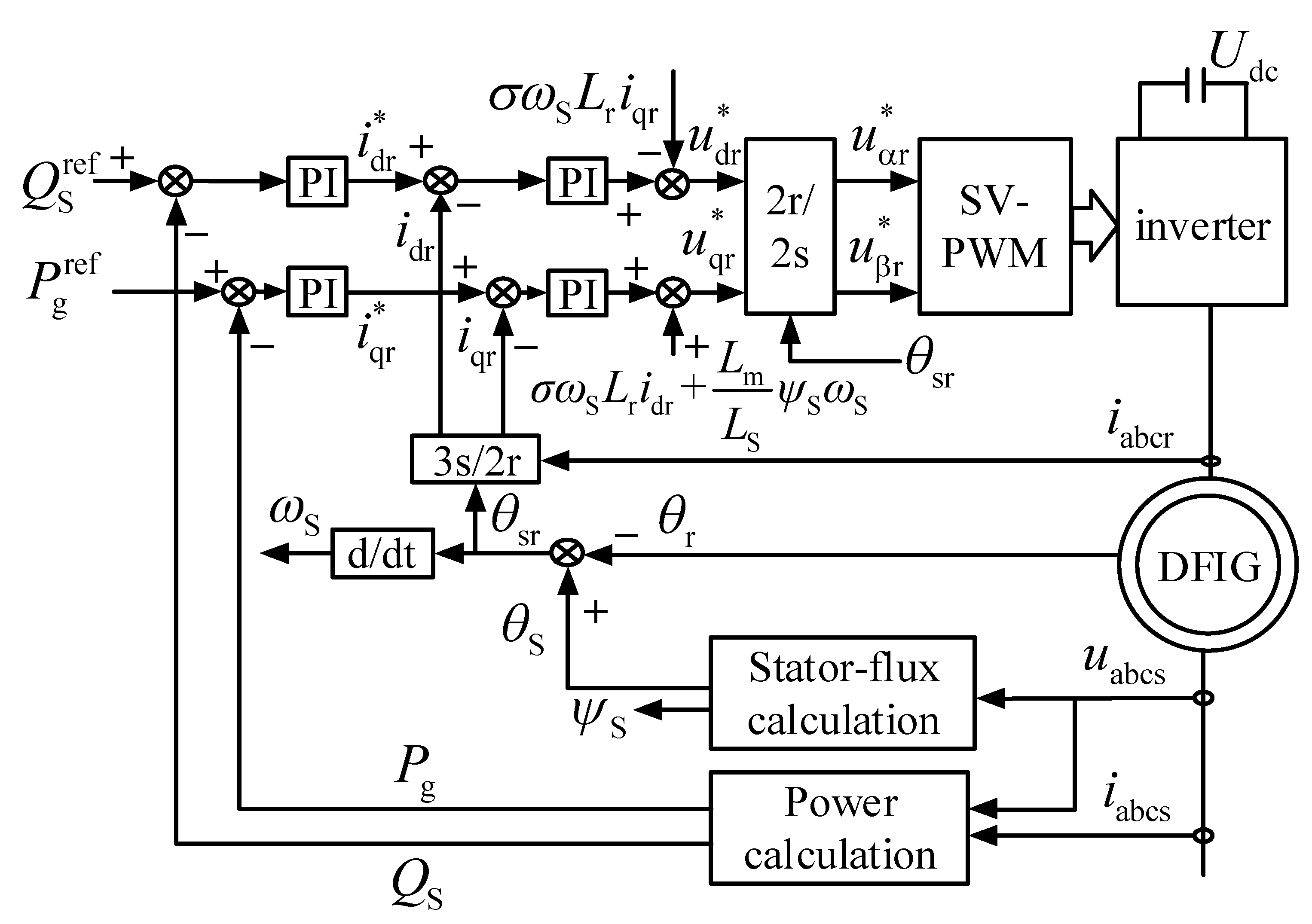
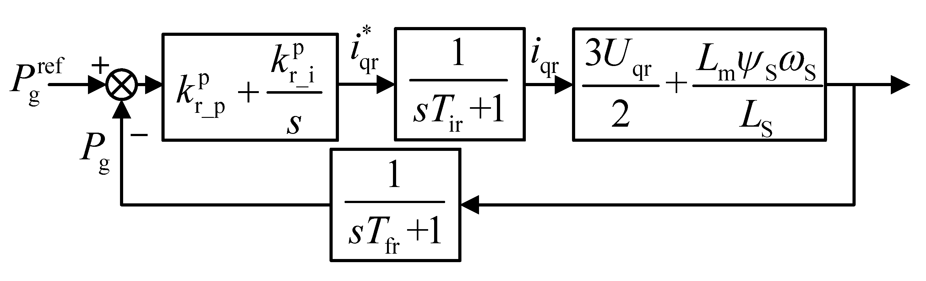
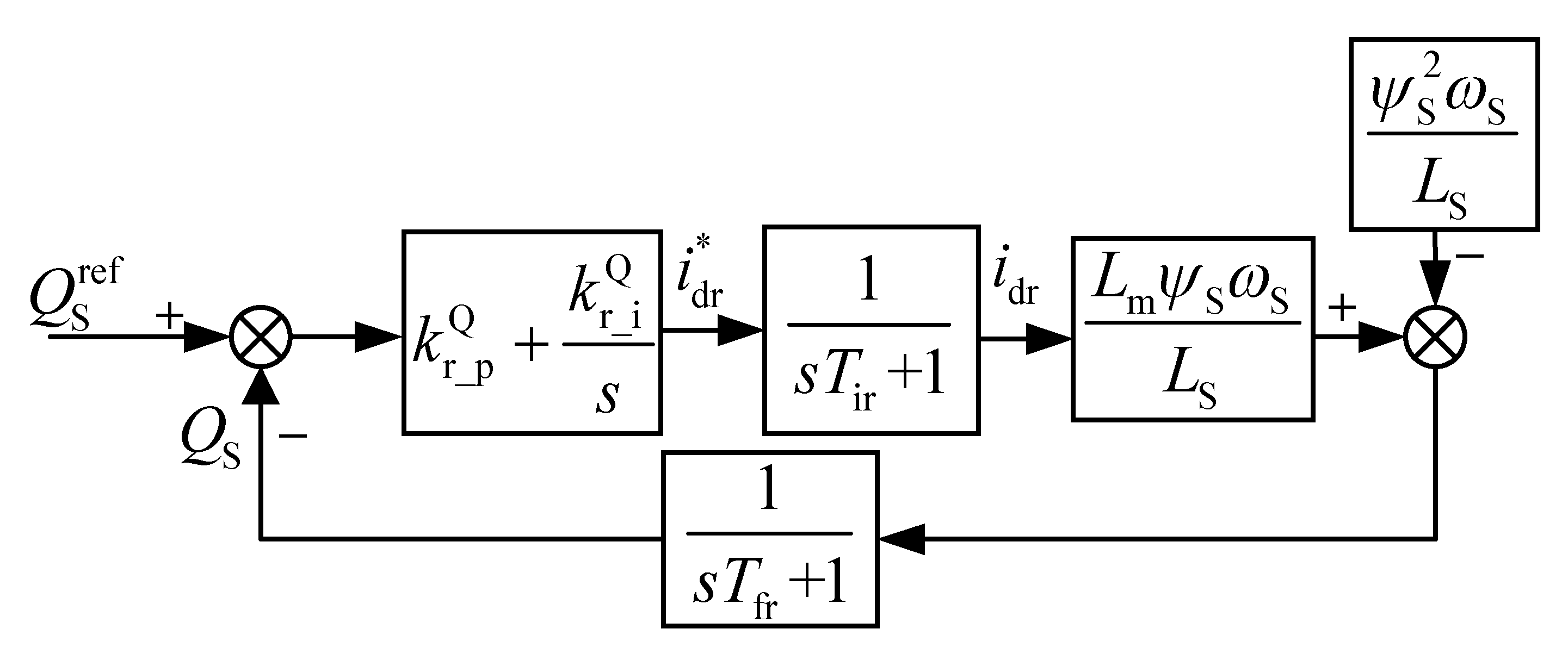
3.1. RSC Model
3.2. GSC Model
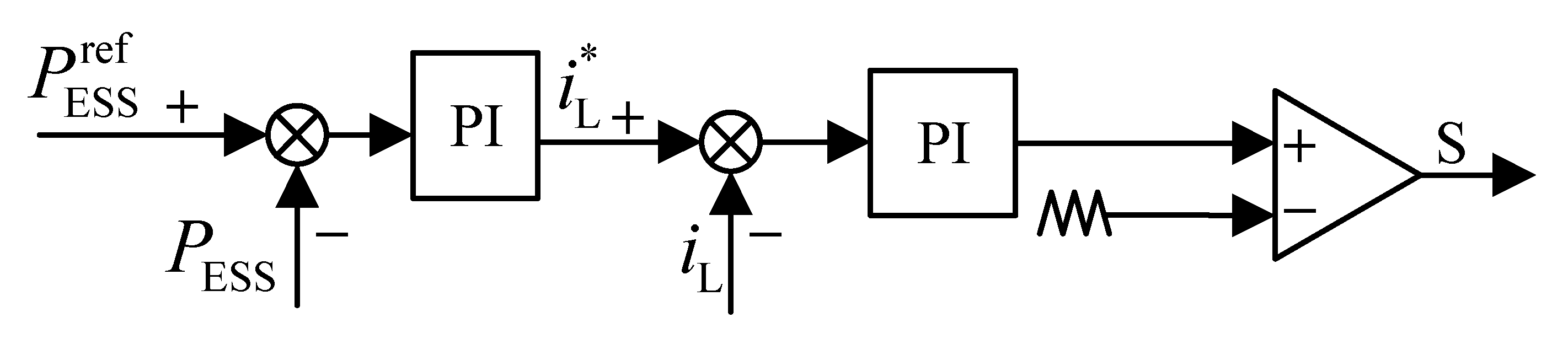
3.3. ESS Model
3.4. WT Model
3.5. Whole System Model
4. MPC Based Coordinated Active and Reactive Power Control for Wind Farm with ESSs
4.1. The First Stage Control
4.1.1. Objective Function
4.1.2. Constraints
4.2. The Second Stage Control
4.2.1. Objective Function
4.2.2. Constraints
5. Case Study
5.1. Test System
5.2. Control Performance
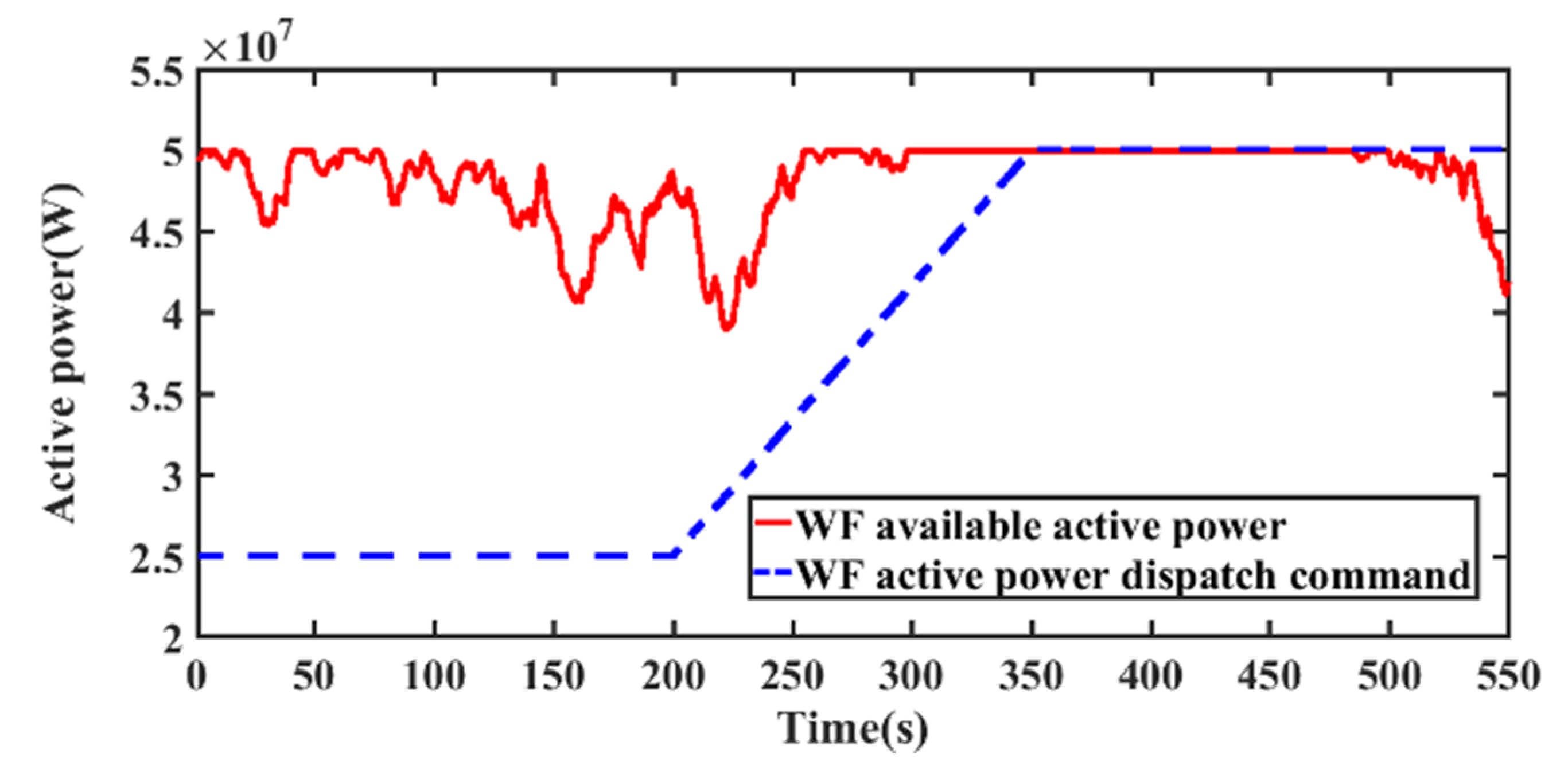
5.2.1. The First Stage Control Performance
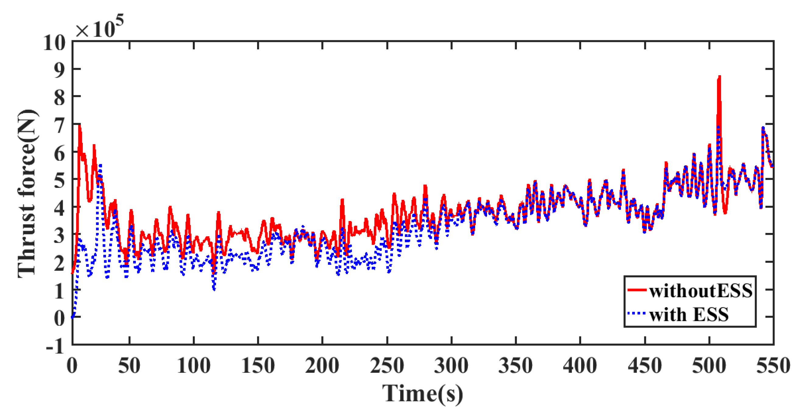
5.2.2. Simulation Analysis of the Second Stage
6. Conclusions
Author Contributions
Funding
Institutional Review Board Statement
Informed Consent Statement
Data Availability Statement
Conflicts of Interest
Nomenclature
| Abbreviations | |
| DFIG | Doubly fed induction generator |
| MPC | Model predictive control |
| WT | Wind turbine |
| WF | Wind farm |
| ESS | Energy storage system |
| GSC | Grid-side converter |
| TSO | Transmission system operator |
| POC | Point of connection |
| RSC | Rotor-side converter |
| SOC | State-of-charge |
| OLTC | On-load tap changer |
| ESU | Energy storage unit |
| Variables | |
| DFIG active power output | |
| QS | DFIG stator reactive power |
| mutual inductance | |
| stator flux | |
| ωS | supply angular speed |
| LS | DFIG stator inductance |
| Uqr | q-axis rotor voltage |
| iqr | rotor q-axis current |
| , , , | proportional gain and integral gain of PI controllers |
| Tir | time constant of current loop |
| Tfr | denote filter time constant |
| Pint | error integral of and Pg, |
| error between and QS. | |
| Qc | GSC reactive power |
| Um | grid phase voltage amplitude |
| , | proportional gain and integral of PI controller |
| Tig | current loop time constant |
| Tfg | GSC filter time constant. |
| error between and QC. | |
| CESS | ESS stored energy |
| CESS,0 | initial energy |
| PESS | charge/discharge power of ESS |
| , | proportional gain and integral of the PI controller |
| UESS | ESU voltage |
| Tid | current loop time constant |
| Tfd | ESS filter time constant |
| ΔCESS, ΔiL, ΔPESS, Δ and Δ | as the incremental value between its current value and the initial value at the operation point |
| error of and PESS | |
| θ | pitch angle |
| K0,K1 | constants |
| Tθ | time constant of pitch servo function |
| Ta | aerodynamic torque |
| Tg | generator torque |
| Kp,Ki | proportional gain and integral gain of pitch controller |
| ωf | generator speed |
| ωg | low-pass filter |
| Tf | filter time constant |
| ηγ | gear box ratio |
| Jr | rotor mass |
| Jg | generator mass |
| Jt | equivalent mass |
| μg | generator efficiency |
| TS | shaft torque |
| Ft | thrust force |
| KβT, KωT, KβF and KωF | are the coefficients obtained the Taylor expansion of TS and Ft at the operating point |
| NP | MPC predictive steps, |
| intermediate level of total ESS capacity | |
| λC,λT,λF | weighting coefficients for the total ESSs energy management variations of TS and Ft |
| NMV | is the number of MV bus |
| predictive incremental voltage of MV bus and WT terminal bus | |
| predictive value of network power losses | |
| λV, λL, λS | weighting coefficients for ObjV, ObjL, ObjS, |
| , | ESS available charging/discharging power |
| / | minimum Var capacity of the DFIG stator and GSC |
| / | maximum Var capacity of the DFIG stator and GSC |
References
- Zhang, D.; Zhang, X.; He, J.; Chai, Q. Offshore wind energy development in China: Current status and future perspective. Renew. Sustain. Energy Rev. 2011, 15, 4673–4684. [Google Scholar] [CrossRef]
- Menezes, D.; Mendes, M.; Almeida, J.A.; Farinha, T. Wind Farm and Resource Datasets: A Comprehensive Survey and Overview. Energies 2020, 13, 4702. [Google Scholar] [CrossRef]
- Hanifi, S.; Liu, X.; Lin, Z.; Lotfian, S. A Critical Review of Wind Power Forecasting Methods—Past, Present and Future. Energies 2020, 13, 5707. [Google Scholar] [CrossRef]
- Perveen, R.; Kishor, N.; Mohanty, S.R. Off-shore wind farm development: Present status and challenges. Renew. Sustain. Energy Rev. 2014, 29, 780–792. [Google Scholar] [CrossRef]
- Mohseni, M.; Islam, S.M. Review of international grid codes for wind power integration: Diversity, technology and a case for global standard. Renew. Sustain. Energy Rev. 2012, 16, 3876–3890. [Google Scholar] [CrossRef]
- Karthikeya, B.R.; Schütt, R.J. Overview of wind park control strategies. IEEE Trans. Sustain. Energy 2014, 5, 416–422. [Google Scholar] [CrossRef]
- Munteanu, I. Optimal Control of Wind Energy Systems: Towards a Global Approach; Springer: London, UK, 2008. [Google Scholar]
- Gasparis, G.; Lio, W.H.; Meng, F. Surrogate Models for Wind Turbine Electrical Power and Fatigue Loads in Wind Farm. Energies 2020, 13, 6360. [Google Scholar] [CrossRef]
- Zhao, H.; Wu, Q.; Guo, Q.; Sun, H.; Xue, Y. Optimal active power control of a wind farm equipped with energy storage system based on distributed model predictive control. IET Gener. Trans. Distri. 2016, 10, 669–677. [Google Scholar] [CrossRef] [Green Version]
- Kim, C.; Muljadi, E.; Chung, C.C. Coordinated Control of Wind Turbine and Energy Storage System for Reducing Wind Power Fluctuation. Energies 2018, 11, 52. [Google Scholar] [CrossRef] [Green Version]
- Yan, G.G.; Wang, Z.B.; Li, J.H.; Li, H.B.; Yang, Y.L. Optimization of Large Scale Energy Storage System for Relaxing Wind Power Centralized Transmission Bottlenecks. Adv. Mater. Res. 2014, 1070, 243–246. [Google Scholar] [CrossRef]
- Meghni, B.; Dib, D.; Azar, A.T. A second-order sliding mode and fuzzy logic control to optimal energy management in wind turbine with battery storage. Neural Comput. Appl. 2016, 28, 1417–1434. [Google Scholar] [CrossRef]
- Qu, L.; Qiao, W. Constant power control of DFIG wind turbines with supercapacitor energy storage. IEEE Trans. Ind. Appl. 2011, 47, 359–367. [Google Scholar] [CrossRef] [Green Version]
- Sarrias, R.; Fernández, L.M.; García, C.A. Coordinate operation of power sources in a doubly-fed induction generator wind turbine/battery hybrid power system. J. Power Source 2012, 205, 354–366. [Google Scholar] [CrossRef]
- Fortmann, J.; Wilch, M.; Koch, F.W.; Erlich, I. A novel centralised wind farm controller utilising voltage control capability of wind turbines. In Proceedings of the 16th PSCC, Glasgow, UK, 14–18 July 2008; pp. 914–919. [Google Scholar]
- Zhao, H.; Wu, Q.; Guo, Q.; Sun, H.; Huang, S.; Xue, Y. Coordinated voltage control of a wind farm based on model predictive control. IEEE Trans. Sustain. Energy 2016, 7, 1440–1451. [Google Scholar] [CrossRef] [Green Version]
- Schönleber, K.; Collados, C.; Pinto, R.T.; Ratés-Palau, S.; Gomis-Bellmunt, O. Optimization-based reactive power control in HVDC-connected wind power plants. Renew. Energy 2017, 109, 500–509. [Google Scholar] [CrossRef] [Green Version]
- Sakamuri, J.N.; Rather, Z.H.; Rimez, J.; Altin, M.; Göksu, Ö.; Cutululis, N.A. Coordinated voltage control in offshore HVDC connected cluster of wind power plants. IEEE Trans. Sustain. Energy 2016, 7, 1592–1601. [Google Scholar] [CrossRef]
- Zhang, B.; Hou, P.; Hu, W.; Soltani, M.; Chen, C.; Chen, Z. A Reactive Power Dispatch Strategy with Loss Minimization for a DFIG Based Wind Farm. IEEE Trans. Sustain. Energy 2017, 7, 914–923. [Google Scholar] [CrossRef]
- Guo, Q.; Sun, H.; Wang, B.; Zhang, B.; Wu, W.; Tang, L. Hierarchical automatic voltage control for integration of large-scale wind power: Design and implementation. Electr. Power Syst. Res. 2015, 120, 234–241. [Google Scholar] [CrossRef]
- Sguarezi Filho, A.J.; de Oliveira Filho, M.E.; Ruppert Filho, E. A predictive power control for wind energy. IEEE Trans. Sustain. Energy 2011, 2, 97–105. [Google Scholar]
- Liu, X.; Kong, X. Nonlinear model predictive control for DFIG based wind power generation. IEEE Trans. Automat. Sci. Eng. 2014, 11, 1046–1055. [Google Scholar] [CrossRef]
- Hu, J.; Zhu, J.; Dorrel, D. Predictive direct power control of doubly fed induction generators under unbalanced grid voltage conditions for power quality improvement. IEEE Trans. Sustain. Energy 2014, 6, 687–695. [Google Scholar] [CrossRef]
- Zhao, H.; Wu, Q.; Wang, J.; Liu, Z.; Shahidehpour, M.; Xue, Y. Combined active power and reactive power control of wind farms based on model predictive control. IEEE Trans. Energy Convers. 2017, 32, 1177–1187. [Google Scholar] [CrossRef] [Green Version]
- Huang, S.; Wu, Q.; Guo, Y.; Lin, Z. Bi-level decentralised active power control for large-scale wind farm cluster. IET Renew. Power Gener. 2018, 12, 1486–1492. [Google Scholar] [CrossRef]
- Guo, Y.; Gao, H.; Wu, Q.; Zhao, H.; Østergaard, J.; Shahidehpour, M. Enhanced Voltage Control of VSC-HVDC Connected Offshore Wind Farms Based on Model Predictive Control. IEEE Trans. Sustain. Energy 2017, 9, 474–487. [Google Scholar] [CrossRef] [Green Version]


Publisher’s Note: MDPI stays neutral with regard to jurisdictional claims in published maps and institutional affiliations. |
© 2021 by the authors. Licensee MDPI, Basel, Switzerland. This article is an open access article distributed under the terms and conditions of the Creative Commons Attribution (CC BY) license (https://creativecommons.org/licenses/by/4.0/).
Share and Cite
Cui, H.; Li, X.; Wu, G.; Song, Y.; Liu, X.; Luo, D. MPC Based Coordinated Active and Reactive Power Control Strategy of DFIG Wind Farm with Distributed ESSs. Energies 2021, 14, 3906. https://doi.org/10.3390/en14133906
Cui H, Li X, Wu G, Song Y, Liu X, Luo D. MPC Based Coordinated Active and Reactive Power Control Strategy of DFIG Wind Farm with Distributed ESSs. Energies. 2021; 14(13):3906. https://doi.org/10.3390/en14133906
Chicago/Turabian StyleCui, Hesong, Xueping Li, Gongping Wu, Yawei Song, Xiao Liu, and Derong Luo. 2021. "MPC Based Coordinated Active and Reactive Power Control Strategy of DFIG Wind Farm with Distributed ESSs" Energies 14, no. 13: 3906. https://doi.org/10.3390/en14133906