Optimization of Costs and Self-Sufficiency for Roof Integrated Photovoltaic Technologies on Residential Buildings

Abstract

It is common practice, in the production of photovoltaic energy to only use the south-exposed roof surface of a building, in order to achieve the maximum production of solar energy while lowering the costs of the energy and the solar technologies. However, using the south-exposed surface of a roof only allows a small quota of the energy demand to be covered. Roof surfaces oriented in other directions could also be used to better cover the energy load profile. The aim of this work is to investigate the benefits, in terms of costs, self-sufficiency and self-consumption, of roof integrated photovoltaic technologies on residential buildings with different orientations. A cost-optimal analysis has been carried out taking into account the economic incentives for a collective self-consumer configuration. It has emerged, from this analysis, that the better the orientation is, the higher the energy security and the lower the energy costs and those for the installation of photovoltaic technologies. In general, the use of south-facing and north-facing roof surfaces for solar energy production has both economic and energy benefits. The self-sufficiency index can on average be increased by 8.5% through the use of photovoltaic installations in two directions on gable roofs, and the maximum level that can be achieved was on average 41.8, 41.5 and 35.7% for small, medium and large condominiums, respectively. Therefore, it could be convenient to exploit all the potential orientations of photovoltaic panels in cities to improve energy security and to provide significant economic benefits for the residential users.

1. Introduction

The energy transition toward more sustainable and resilient energy management, through the use of renewable energy sources, has become one of the principal challenges of cities today [1,2,3]. In densely built cities, the only renewable energy source that can be exploited is often solar energy [4]. North-facing roof areas are usually excluded from roof integrated photovoltaic (PV) technologies in the analysis of the technical potential [5]. Moreover, the various criteria used to evaluate the suitability of roofs can lead to significantly different results [6]. Geographic information systems (GISs) are tools that are commonly used to evaluate the PV potential, and they are able to investigate the solar potential from the building scale to the city scale [7,8,9,10,11,12]. One of the limits to the promotion of solar technologies is related to the investment costs [13,14]. With the introduction of the concept of energy community, it is possible to promote the use of PV technologies as a collective self-consumption means as it reduces the investment and energy costs [15]. Italian legislation has recently introduced two configurations for sharing renewable electricity: the collective self-consumer configuration and the renewable energy community one. Economic incentives have been introduced for the promotion of energy communities, and have also been extended to the installation of such technologies as storage systems [16]. Benefits are obtained from the establishment of energy communities, not only due to the smaller amount of energy that is taken from the grid, but also to the amount of energy that can be produced and consumed simultaneously at the local level. Through the configuration of a collective self-consumer, these incentives can promote the use of solar technologies in cities. Two indicators that are used to investigate the technical-economic feasibility of an energy community are the self-consumption index (SCI) and the self-sufficiency index (SSI) [16,17,18]. In this work, these indicators have been used to assess the balance between electrical consumption and PV production.

1.1. Research Gap

For many years, studies that have investigated solar energy in cities have usually only considered the south-facing roof surfaces of buildings for producing energy from PV technologies [13,19,20,21,22,23,24]. Since the only renewable energy source available in densely built cities is usually solar energy, there is a need to exploit the full potential of a roof, but the question is whether this is convenient from an economic point of view.

There are relatively few studies regarding the use of different orientations for the production of energy from PV panels. Azaioud et al. [25] investigated the benefits of PV installations using different orientations, and not only the southern (S) one. They confirmed that energy benefits can be achieved, such as the reduction of the electricity peak and improvements to the SCI and SSI, by resorting to multiple orientations. In [26], the authors analyzed the combination of East (E) and West (W) orientations for PV production with respect to the S one. The authors found that it is possible to reach a higher level of self-consumption and a greater degree of self-sufficiency for an E-W orientation, while the electricity costs are lower for E-W and SE-SW combinations. Lahnaoui et al. [27] confirmed that since the optimum PV orientation depends to a great extent on the hourly load profile of the users, the best solution is not always the use of South-exposed roof surfaces. Mainzer et al. [28] analyzed the PV potential for residential users, taking into account a quota of north-facing roof areas that did not reduce the technical potential (even though the yield from these surfaces is lower). In [29], the authors evaluated the share of solar radiation from differently oriented surfaces. They found, regarding their seasonal analysis, that the north-facing surface had higher daily average solar radiation energy than the south-facing plane. Collectively, these studies outline a potential for the use of non-south oriented surfaces.

1.2. Research Objective

This work critically examines not only the energy benefits of using different orientations for PV technologies, but also investigates the economic costs. It provides new insights into the optimization of the costs and self-sufficiency of roof integrated PV technologies on residential buildings by using multiple orientations of roofs, and it has found, thanks to the economic incentives for collective self-consumer configurations [16], that it is possible to promote the use of PV technologies with low energy costs and a high level of the self-sufficiency index (SSI).

The research focuses on whether energy and economic benefits can be achieved by using two directions for PV installation on gable roofs for residential users configured as collective-self consumers. The presented methodology was applied to the city of Turin, Italy. In this city, only the roof areas with a predominantly south facing orientation (i.e., better-exposed roof surfaces) have generally been used for PV production. Given that the only renewable source that can be exploited is solar energy, this paper investigates whether it is possible to improve energy security and increase self-sufficiency by also using north-exposed roof surfaces (e.g., north, northeast or northwest facing orientations, considered as poorly-exposed roof surfaces). The residential sector has been analyzed in this work, since the hourly load profile is compatible with PV production. Seven residential buildings have been investigated and the impact of the use of two directions for PV installation has been evaluated considering and not considering the space cooling load.

The remaining part of the paper proceeds as follows: Section 2 describes the input data and the methodology used to investigate the PV potential and hourly load profile; Section 3 presents the case study and the residential buildings selected for the analysis; the main findings on SCI, SSI and a cost-optimal analysis are highlighted in Section 4; and the last two sections are dedicated to the discussion, conclusion and future developments.

2. Materials and Methods

This section shows the procedure that was used to assess the energy productivity from solar technologies (Section 2.1), the models used to quantify the hourly load profile of residential buildings (Section 2.2) and the cost-optimal analysis applied to identify the optimal configuration of PV technologies, in terms of costs and self-sufficiency (Section 2.3). The main phases of this work were:

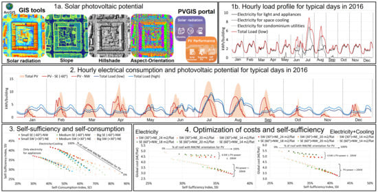
• The processing of input data: the solar PV potential and the annual load profiles with hourly resolution were assessed for seven typical residential users through the use of GIS tools and the PVGIS portal.
• An assessment of the energy balance and the energy performance through two indicators: the SCI and SSI.
• Different scenarios were investigated for the cost-optimal analysis considering investment costs and energy costs. The economic incentive for the ‘collective self-consumer’ configuration was taken into account. Such a configuration considers producing renewable electricity for the residents’ own consumption and storing or selling the overproduced amount to the grid.

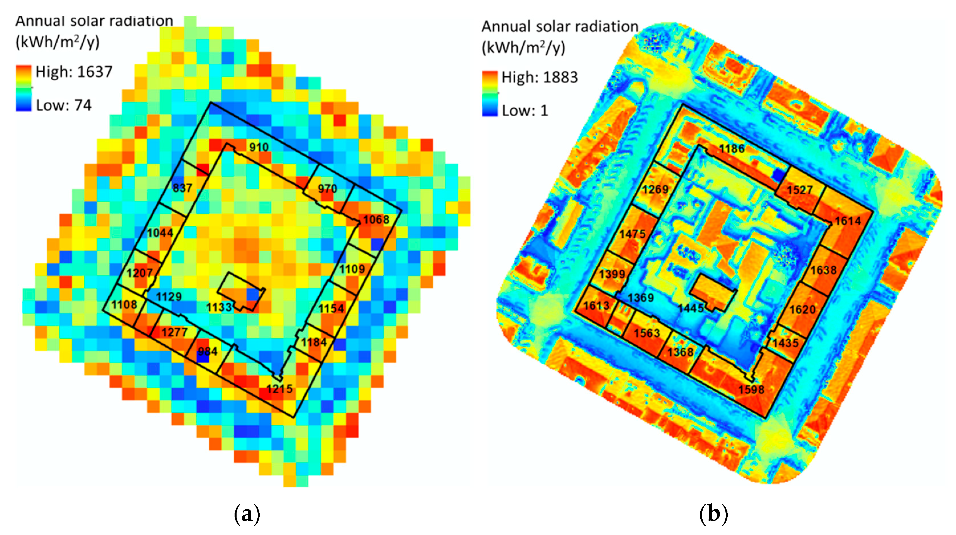
2.1. Solar Photovoltaic Potential

This section shows the methodology used to assess the energy productivity from solar technologies (photovoltaic modules) at an urban level using GIS tools and the PVGIS portal (https://re.jrc.ec.europa.eu/pvg_tools/en/#PVP (accessed on June 2021)). The solar PV potential of roofs was quantified at a building level for a neighborhood in the city of Turin by analyzing the available roof area, taking into account several criteria [8,30,31,32,33]: the shape of the roof (i.e., area and slope), the presence of disturbing elements, the roof orientation, the quota of solar radiation, as a function of the local climate conditions, and the built environment, energy and environmental regulations, heritage and aesthetic criteria.

With the support of GIS tools–ArcGIS 10.7 (ESRI) was used in this work–the geometrical characteristics of residential buildings and the shape of the roofs were assessed using the footprint area (from the Municipal Technical Map of the city of Turin) and a Digital Surface Model (DSM), which represents the earth’s surface and includes buildings and vegetation. The average slope of the roofing elements of the buildings was calculated with the ‘Slope’ tool. The disturbing elements (i.e., dormers and antennas) were identified using the ‘Zonal Statistics’ tool, which calculates statistic values of raster data for each roof surface. The disturbance percentage of each roof was identified from the standard deviation using orthophotos, an annual solar radiation analysis and a hillshade analysis. The orientation of the roofs was analyzed using two tools:

• The ‘Aspect’ tool, which uses the DSM as input data and is able to identify the downslope direction. The simulation times vary according to the accuracy of the DSM, and the times are quite long, for a DSM of 0.5 m (high precision level), to do a city-scale analysis. However, it is possible to reduce the times by using a DSM of 5 m (medium precision level), but the results are obviously less accurate. The output values range from 0° to 360°, where 0° and 360° correspond to the North direction and 180° to the South direction (flat areas with no downslope direction are given a value of −1). In this work, the outputs were processed and the roof surfaces were classified according to the orientation.
• The ‘Calculate Polygon Main Angle’ tool, which uses a footprint area as input data. This tool is able to calculate the dominant angles of input buildings and assign a value to them. In this case, the simulation times are much shorter than those of the ‘Aspect’ tool, because it only returns the prevailing orientation. It is good practice to choose the correct tool, depending on the type of data that are needed, to optimize and make the methodology easily applicable. In this work, both tools were used to evaluate the exposed surface of the roof.

The annual, monthly and hourly solar radiation values were calculated at a building level with ArcGIS using the ‘Area Solar Radiation’ tool (‘Points solar radiation’ is a similar tool) to establish the solar PV potential. In this work, input data of different accuracy levels were considered in order to evaluate the simulation precision and the simulation time. The urban built environment was assessed using two DSMs with different accuracies: the first one was less accurate, with a precision of 5 m (duration of the simulation time for a block of buildings with a dimension of 150 m × 150 m: 7 s), while the other one was more accurate, with a precision of 0.5 m (duration of the simulation time for a block of buildings: 25 s). The local climate radiation refers to two parameters: (i) the atmospheric transparency assessed according to the linke turbidity factor (τ, -), elaborated using Meteonorm software (https://meteonorm.com/en/ (accessed on April 2021)); (ii) the ratio of diffuse radiation to global radiation (ω, -), released from the PVGIS portal (https://ec.europa.eu/jrc/en/pvgis (accessed on June 2021)). The solar analysis was performed for a whole year at a monthly interval (the year 2016 was considered a typical meteorological year according to the period from 2010 to 2020 [18]). The solar analysis considered three different models of sun and sky more or less precise in terms of time periods: with annual, seasonal (three intervals) and monthly characteristics.

Table 1. Sun and sky data to evaluate the solar energy radiation (year 2016—Turin, Italy).

Months	Monthly Analysis		Seasonal Analysis		Annual Analysis
	ω	τ	ω	τ	ω	τ
January	0.58	0.29	0.58	0.32	0.54	0.47
February	0.68	0.31
December	0.48	0.35
March	0.69	0.44	0.57	0.47
April	0.63	0.51
May	0.60	0.53
September	0.41	0.57
October	0.42	0.51
November	0.65	0.28
June	0.58	0.54	0.44	0.60
July	0.39	0.62
August	0.35	0.63

shows the solar radiation parameters for these three levels of analysis according to the year 2016. For the simulations the ‘Area solar radiation’ tool of ArcGIS was used with the following parameters: 8 zenith divisions, 8 azimuth divisions and a ‘Standard overcast sky’ for the diffuse model (i.e., diffuse radiation varies with zenith angle).

Figure 1 shows the annual solar radiation (kWh/m²/year) obtained at a block of building scale using a DSM with a precision of 5 m and annual average radiation parameters (one simulation to analyze the whole year, with a monthly interval output), and using a DSM with a precision of 0.5 m and monthly average sun and sky data (12 simulations to analyze the whole year, one per month). In this type of analysis, the more accurate the input data, i.e., DSM of 0.5 m and monthly sky and sun data, the better the results describe the real conditions. In Figure 1 the average numerical value of annual solar radiation incident on the roof of the buildings has been represented. The accuracy of the outputs was improved by using more accurate input data (Figure 1b). It is possible to observe that with a coarser grain (e.g., DSM of 5 m) the sunniest areas are together with areas that receive less solar radiation, and therefore, for example, roofs are generally less sunny (because the grid includes not only the roof but also part of the surrounding areas). In general, using a DSM with low precision and annual parameters, simulations are less accurate and tended to underestimate the solar radiation values (especially during the summer months).

These solar radiation data processed in ArcGIS were compared with the data developed from the PVGIS portal and with data recorded by a weather station located in the city of Turin. Figure 2 compares the monthly horizontal irradiation data (kWh/m²/month) produced using different input data and different types of simulation and tools (ArcGIS vs. PVGIS). The data indicated in the table show the number of simulations made as a function of the input data, the simulation times, and the annual mean absolute percentage error (MAPE). The MAPE was calculated using as reference data the more accurate simulations made with the DSM of 0.5 m and monthly sun and sky data. The ArcGIS simulations, made with monthly climatic data (12 simulations), showed a higher monthly variation than those made with the seasonal (three simulations) or annual (one simulation) sun and sky data.

The solar irradiation values resulting by the 0.5 m DSM were higher than those of the 5 m DSM. The data developed from PVGIS were sufficiently accurate, compared with the ArcGIS results. The MAPE shows that the PVGIS results are reasonably accurate with a MAPE of 11%.

In summary, the simulations made in ArcGIS allowed more accurate results to be obtained with higher solar irradiation values during the summer and lower ones during the winter. This is because the analysis was performed considering the monthly climatic conditions and the real characteristics of the territory with a very high precision (DSM of 0.5 m). Less accurate data were obtained from the simulations that used seasonal/annual climatic conditions (without monthly variation), PVGIS data (which refers to solar energy models and data from weather stations) and weather station measurements (with climatic data records referring to a single point on the territory).

Subsequently, an analysis was carried out to evaluate the solar radiation according to the different orientations and inclinations of the rooftop of the buildings in Turin. Figure 3 shows an example of the comparison of the monthly solar radiation (kWh/m²/month) considering four orientations: SE, with an azimuth of −60° (Figure 3a), SW, with an azimuth of +30° (Figure 3b), NW, with an azimuth of +120° (Figure 3c), and NE, with an azimuth of −150° (Figure 3d).

These are the typical orientations of buildings in Turin. The monthly data produced using DSMs of 0.5 and 5 m and monthly radiation parameters were compared with data developed from the PVGIS portal. The annual relative error (RE) in the graphs is indicated to compare the PVGIS data with ArcGIS data.

In general, it can be observed a more significant difference between the months using the monthly sun and sky data. Furthermore, depending on the orientation, the solar radiation values are greater, with azimuths of +30° and −60°, and this trend is obtained for all the analyses. PVGIS data are able to capture the differences as a function of orientations and are reasonably accurate, although are less sensitive to monthly variation. However, compared PVGIS data to the data processed using ArcGIS tools, have an average relative error of ±20%.

Therefore, several methods and tools of various degrees of accuracy that can be used to evaluate the solar PV potential of roofs are available. The simulation times and data processing times of ArcGIS are quite high, depending on the extent of the analyzed area and on the accuracy of the input data (i.e., DSM precision and radiation parameters). Processing with PVGIS is fast and simple, and it is possible to collect both hourly solar radiation and PV performance values.

One of the main strengths of ArcGIS tools is that they provide outputs which describe the real conditions on a city scale with greater accuracy with respect to other tools, such as PVGIS. The only real weakness is that, in carrying out this type of analysis, the more precise the input data are (a DSM of 0.5 m and monthly climatic conditions), the more expensive the data processing is and the longer the time required for simulations, and especially for processing the outputs, is, too. The results presented in this section refer to a small area of the city of Turin (with a dimension of 150 m × 150 m), if the analysis was carried out for the whole city, the collection and processing of the data would have required a significant effort. This is the main reason why other tools such as PVGIS are often used. They have limitations in terms of the correctness of the data, but are still reasonably accurate and the processing is very simple and fast. As for the data from weather stations, they are real data measured at a specific point in the territory, therefore, depending on the location of the weather station, very different results may be obtained. This can significantly affect city-scale analyses.

In this work, ArcGIS tools were used to accurately describe each surface of the urban environments, and the resulting characteristics were used as input data in PVGIS. Then, hourly data processed from the PVGIS portal were considered accurate enough to perform the analysis. A georeferenced database was created in this work, using GIS tools, in order to evaluate the rooftop area that could be used for the installation of PV technologies, considering different orientations, inclinations and the presence of disturbing elements on the roofs. The analysis was performed on seven residential buildings located in a neighborhood in Turin.

Since the energy production with the PVGIS portal is considered sufficiently accurate, the hourly solar PV potential was quantified for one year using this portal, considering an inclination of PV modules of 25°. For these simulations, polycrystalline silicon modules were used with a module energy conversion efficiency in standard test conditions of 26.7% ± 0.5 [34]; PVGIS calculates the efficiency variation according to solar radiation intensity and spectrum, module temperature and wind speed. Moreover, PVGIS considers also an average value of 14% of energy losses by the cables and the inverter, and due to dirt and snow on the modules. Different scenarios were investigated, according to the maximum installable power for each roof, to identify the optimal dimension of PV modules.

2.2. Hourly Load Profile

This section shows details of the methodology that was used to assess the hourly load profile of residential buildings. The energy consumption is composed of: electricity for light and appliances, electricity for space cooling, and electricity for condominium utilities (i.e., elevators).

2.2.1. Electricity for Light and Appliances

The hourly electricity consumptions for light and appliances of the residential users were calculated considering monthly electrical data measured for two consecutive years (2016 and 2017) for over 100 residential buildings located in a neighborhood in Turin [18]. The normal distributions were investigated in order to evaluate the frequency distribution of the annual consumption of the residential users for the year 2016. Two statistical tests were run in conjunction with the distributions to observe the trend of the annual consumption of the buildings and to discard any anomalous data: the Kolmogorov-Smirnov (KS) and chi-squared (χ²) tests.

Figure 4 shows the normal distribution of the annual measured data of 107 residential users analyzed for the year 2016, and both KS and χ² were verified. The median annual electricity consumption in this neighborhood is 1917 kWh/user/year, and two types of residential consumers were identified: low-consumer with 1652 kWh/user/year (median minus the standard deviation) and high-consumer with 2182 kWh/user/year (median plus the standard deviation). In this work, the number of users in each building being known, it was possible to quantify the total electrical consumption for low-consumption and high-consumption users.

The seasonal hourly profile was identified using the hourly profiles of some typical days in the winter, spring, summer and autumn periods as a reference, and distinguishing between working and non-working days. The hourly profiles refer to over 400 families in the Piedmont Region with 2.15 components per family [35]. Therefore, from the monthly measured data, and the hourly profiles for one year being known, it was possible to calculate the hourly electricity for light and appliances for the year 2016 for each residential building.

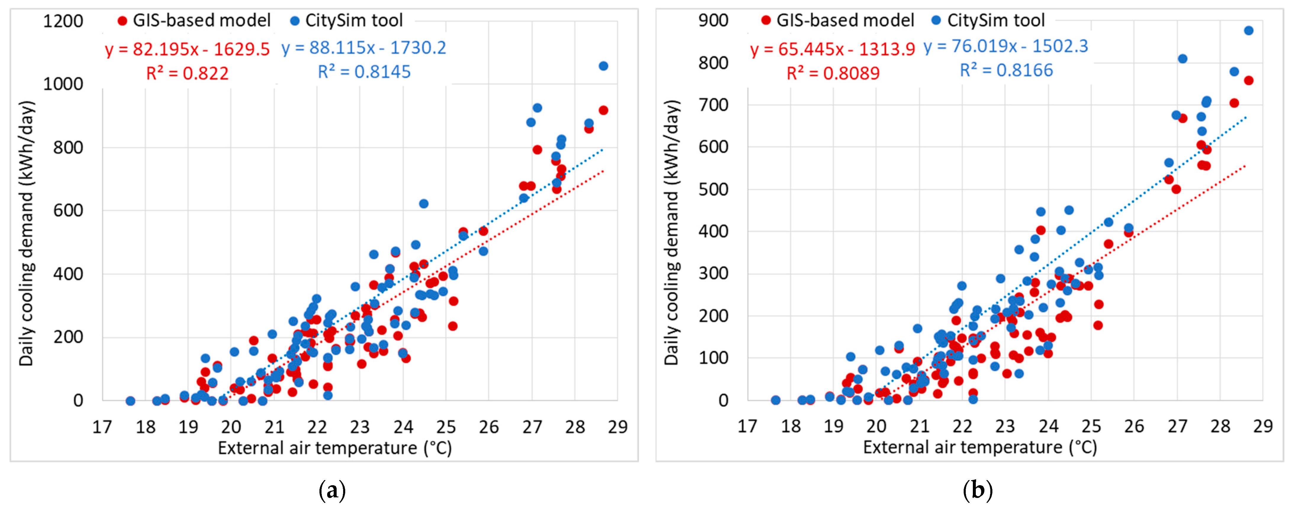
2.2.2. Electricity for Space Cooling

The hourly electricity for space cooling of the residential buildings was quantified by applying a GIS-based engineering model. This model is a dynamic thermal balance of buildings that was adapted to a neighborhood scale. This GIS-based model is a lumped parameter model, based on three thermodynamic systems: the opaque envelope, the glazing components, and the inside part of the building (internal structures, air, occupants and furniture) [36]. The model was validated, according to a previous work [37], through a comparison of the results, using the CitySim tool and the ISO 52016 standard [38].

Figure 5 shows an example of the hourly cooling demands for the five typical summer days, simulated for two residential buildings in the neighborhood analyzed in this work. It can be observed that the hourly cooling profiles (continuous line) have a similar trend related to the solar irradiation (dashed line). The results of the GIS-based model and the CitySim tool are very close to each other. However, the hourly ISO 52016 method simulates a higher consumption than the other two tools, especially for May and September. The daily absolute relative error for these selected days, according to the CitySim data, is on average 14% (median 7%).

Figure 6 shows the daily energy demand for space cooling of the two buildings described in Figure 5. As expected, the daily energy demand (kWh/day) increases as the daily external air temperature increases. However, as these models are tools that are used to perform simulations at a district scale, and not at a building scale, a 20% margin of error is compatible with neighborhood-scale analyses.

The hourly electricity for space cooling was quantified by assuming an air-to-air electric heat pump of 35 kW with an energy efficiency ratio (EER) that varies from 6.3 (when the external air temperature is 20 °C) to 4.3 (when the outdoor air temperature is 35 °C).

According to the EER requirements indicated in Italian Ministerial Decree 26/6/15 “Application of energy performance calculation methods and definition of the prescriptions and minimum requirements of buildings" (and subsequent amendments and additions), the correlations between EER and the external air temperature were identified using heat pumps of 25 and 35 kW, which are typical characteristics of the heat pumps available on the market (

Table 2. Correlations between EER (considering a load factor of 100%) and the external air temperature (T_ae, °C) of a typical air-to-air electric heat pump available on the market.

Heat Pump Power	EER Linear Correlation	R2
25 kW	−0.1616 ∙ Tae + 10.774	0.998
35 kW	−0.1356 ∙ Tae + 8.989	0.998

).

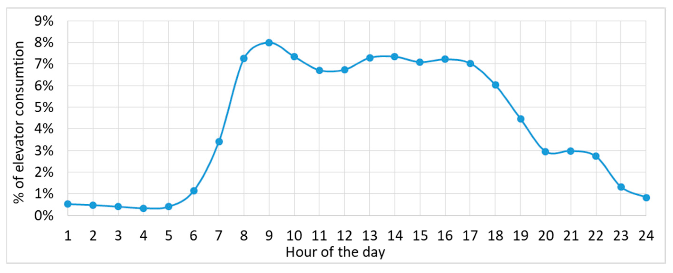
2.2.3. Electricity for Condominium Utilities

In order to calculate the total load of a typical residential building, the electricity consumption of the condominium was also considered in addition to the electricity consumption for light, appliances and space cooling of the flats. The quota of energy used by the elevators was quantified for residential users to calculate the electricity consumed for condominium utilities. In Europe, elevators typically use 3–8% of the overall electricity consumption of a building [39]. This percentage mainly depends on the type of users and on the shape of the building (e.g., the number of floors and number of flats) [40,41].

In this work, taking into account the typology of the residential buildings, an average value of 5.5% was used to quantify the consumption of elevators. Following [42], the daily demand profile with a one-hour resolution was used to identify the hourly load profile of the elevators in the residential buildings. The differences in these energy consumptions between weekdays and holidays are minimal, therefore, only one profile was considered for the entire week. A typical hourly profile of a residential building is shown in Figure 7.

2.3. Energy Indexes and Cost-Optimal Analysis

Firstly, the balance between the electrical consumption and PV production was investigated in order to examine the self-consumption and the self-sufficiency of residential users utilizing all the potential PV surfaces oriented in different directions. The variables considered to analyze the energy balance were:

• Total production (TP), which is the local energy production from new renewable energy source power plants, in our case PV plants;
• Total energy consumption (TC), which is the total energy demand of all the consumers, according to a collective self-consumer configuration;
• Uncovered demand (UD), which is the share of energy consumption that is not satisfied by the produced local energy and which must be withdrawn from the national grid;
• Over-production (OP), which is the share of energy that is not instantly self-consumed as the produced energy is greater than the energy demand: OP = TP − TC);
• Self-consumption (SC), which is the share of energy instantly self-consumed by each user (called prosumer) or, in other words, the energy produced that is used locally: SC = TP − OP or TC − UD or min (TP; TC).

Self-consumption and self-sufficiency were investigated by two indexes considering the annual data with an hourly time step calculation: (i) SCI, which is the ratio between SC and TP; (ii) and SSI, which is the ratio between SC and TC.

Secondly, a cost-optimal analysis was performed to optimize the costs and self-sufficiency of roof integrated PV technologies on residential buildings, taking into account the economic incentives for the collective self-consumer configuration [16,18]. The global cost ($C_G$) of the cost-optimal analysis was calculated for different PV configurations according to Equation (1). In this work, the cost-optimal analysis was performed considering a period of 20 years.

$$C_G=C_I+{\displaystyle \sum }_{i=1}^{\tau }\left(C_{E,i}·R_{d\left(i\right)}\right)$$

(1)

where:

• $C_I$ is the initial investment cost, and in this work it refers to a cost of PV installation equal to (https://www.solareb2b.it/documenti/ (accessed on March 2021), in Italian):

  -

  1000 €/kW_p, if the installed PV power (P) > 20 kW;

  -

  1600 €/kW_p, if 6 kW ≤ P ≤ 20 kW;

  -

  2000 €/kW_p, if P < 6 kW.

• $C_{E,i}$ is the annual energy cost at year $i$, and it was calculated taking in account all the expenses for the energy taken from the grid (i.e., UD), as well as all the revenues generated by the sale of the energy to the grid (i.e., SC and OP). The average cost of the electricity taken from the grid was 0.22 €/kWh for residential users and it was applied to the UD share to calculate the expenses. The revenues were calculated considering the economic incentive for the collective self-consumer configuration in a condominium, which lasts 20 years, and were described as follows:

  -

  +0.10956 €/kWh to be applied to the SC share;

  -

  +0.1 €/kWh to be applied to the OP share.

• $R_{d\left(i\right)}$ is the discount factor at year $i$ was considered and is equal to the 2%.

3. Case Study

The methodology presented in Section 2 was applied to seven typical residential buildings with different dimensions and orientations located in a neighborhood in Turin, Italy. The climate is continental and temperate, with 2648 °C heating degree days at 20 °C and 84 °C cooling degree days at 26 °C mainly concentrated in June, July and August (according to the UNI 10349-3:2016 Standard). About 80% of the buildings in the city are residential, and are mainly large and compact condominiums [32]. The orientation of the buildings was analyzed with GIS tools using a DSM with a precision of 0.5 m and the building footprint according to Section 2.1.

Figure 8 shows the roof surfaces (m²) as a function of the orientation, distinguishing between all the users (i.e., residential, industrial, municipal and tertiary) and residential users. A large number of the roofs are gable roofs with two prevalent orientations: SE, with the azimuth of −60° (16% of the total roof areas) and SW, with the azimuth of +30° (19% of the total roof areas). The prevalent roof pitch angle of the residential buildings is 25° and ranges from 45° to 15° for the gable and pitched roofs.

3.1. Selection of the Residential Buildings

About 90% of the buildings in the analyzed neighborhood are compact residential condominiums, the number of components per family is 2.03 and the average annual electrical consumption for light and appliances is 1928 kWh/user (according to the data measured for 2016). Seven condominiums were selected according to their orientations, dimensions (i.e., small, medium or large condominiums) and the geometrical characteristics (e.g., roof slope). In Turin, there are about 37,700 residential buildings with gable and pitched roofs and the slope of the roofs is mainly 25°, with a standard deviation of 3.77°. The seven selected residential buildings have a slope that varies between 23 and 27°. These buildings are typical of the building heritage of the historical center of the city.

Table 3. Characteristics of the seven typical residential buildings in the considered area.

Building ID	Azimuth	Dimension	No. of Flats	No. of Floors	Roof Area	Total PV Area *	PV Area by No. of Flats
	(°)	(-)	(-)	(-)	(m2)	(m2)	(m2/Flat)
30	SE = −60; NW = +120	Small	10	5	210	SE = 91; NW = 87	18
91		Medium	12	5	283	SE = 156; NW = 149	20
211		Large	22	6	359	SE = 150; NW = 144	14
140	SW = +30; NE = −150	Small	10	5	285	SW = 122; NE = 120	24
258		Medium	12	5	280	SW = 125; NE = 113	20
199		Large	22	6	379	SW = 150; NE = 172	14
153	SE = −45; NW = +135	Medium	12	4	275	SE = 104; NW = 130	20

* The total photovoltaic (PV) area considers a presence of disturbing elements equal to 15% of the roof area.

shows the main characteristics of the selected buildings:

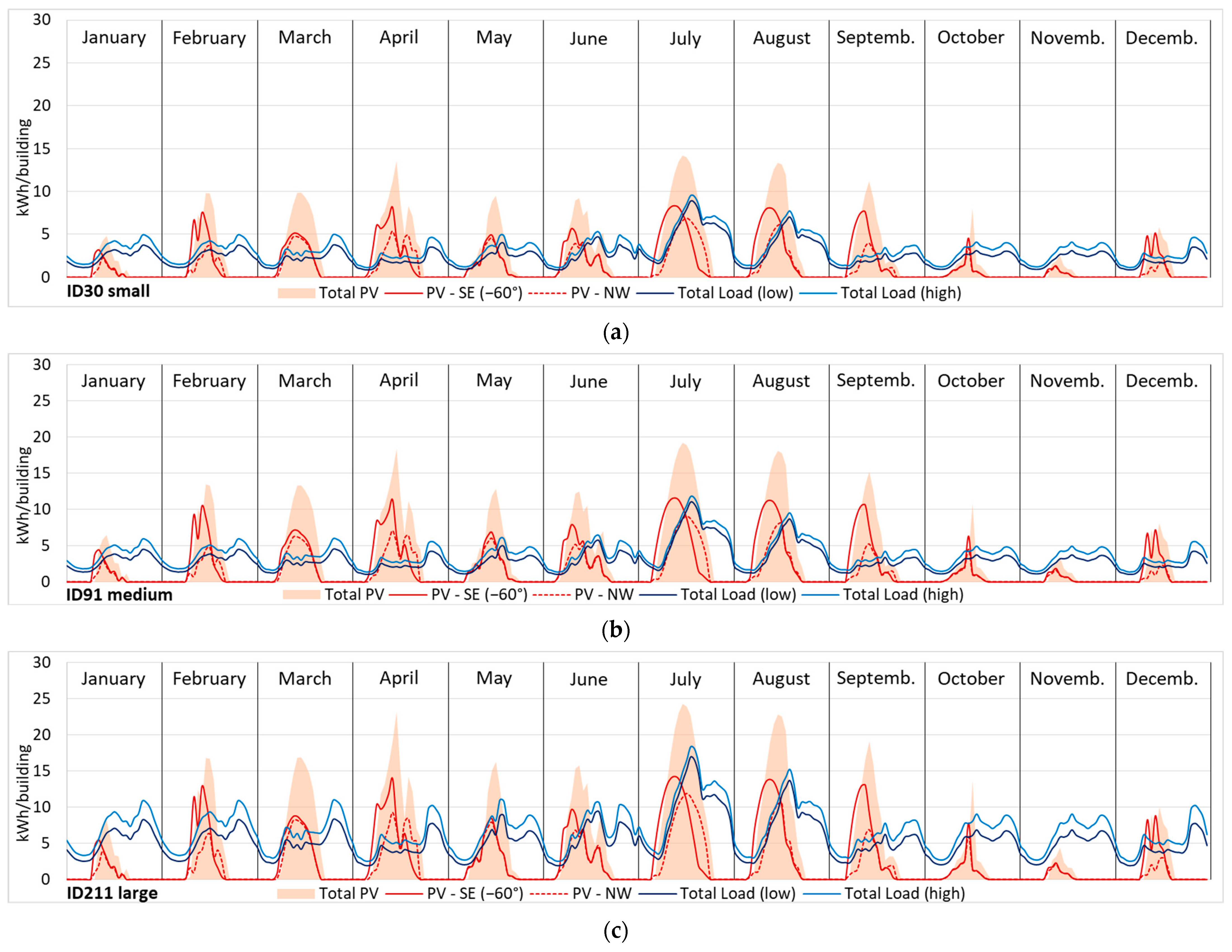
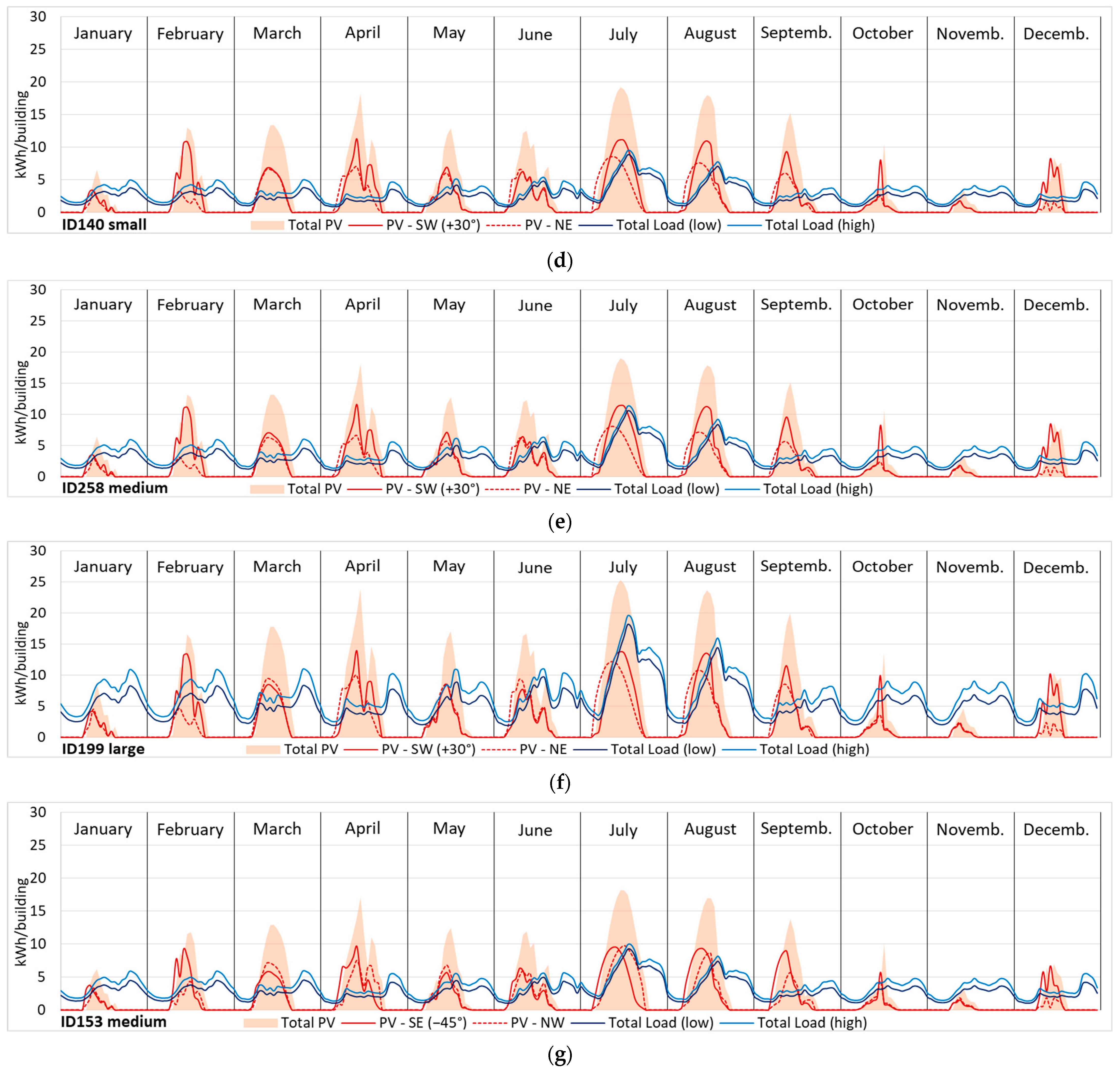
• Small condominiums with 10 flats per building over 5 floors, and the PV area per number of flats varies from 18 to 24 m²/flat;
• Medium condominiums with 12 flats per building over 4–5 floors, a total roof area of about 280 m² and a PV area of 20 m²/flat;
• Large condominiums with 22 flats per building over 6 floors, a total roof area of about 370 m² and a PV area of 14 m²/flat.

The PV area per number of flats is an interesting indicator to describe the maximum PV potential for each family.

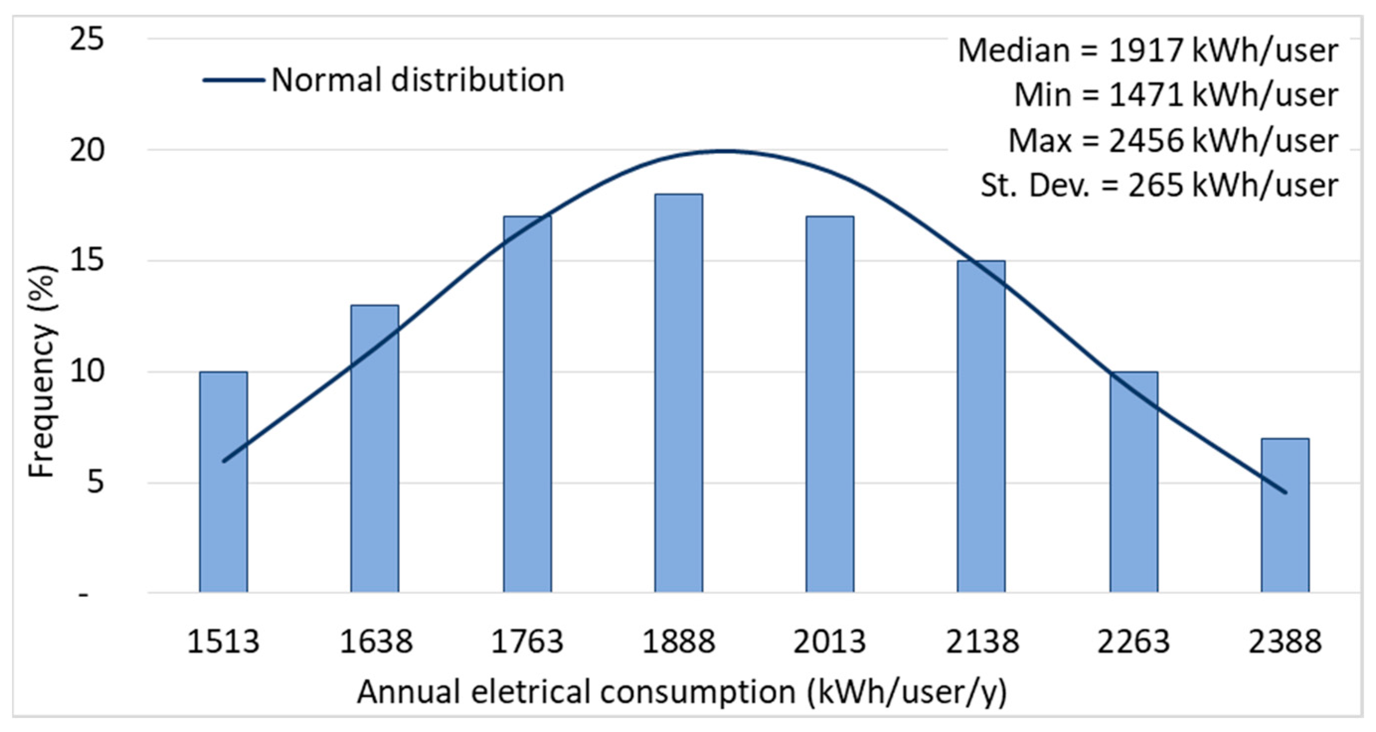
3.2. Electrical Consumption and Photovoltaic Potential

As mentioned in Section 2.2, the hourly load profile takes into account the quota for light and appliances, the quota for space cooling, and the quota for condominium utilities. Two types of residential consumers were investigated regarding the electricity for light and appliances: a low-consumer with 1652 kWh/user/year and a high-consumer with 2182 kWh/user/year. The electricity for space cooling was quantified for each building by applying the GIS-based engineering model taking into account the local climate conditions for the year 2016. The electricity for condominium utilities was quantified considering that the elevator uses 5.5% of the overall electricity consumption of the condominium.

Figure 9 shows the hourly profiles of the total load, distinguishing between low-level consumers and high-level consumers, and the total PV production distinguishing between the two orientations for 12 typical days, each of which is representative of a specific month for the year 2016. It can be observed that in all the cases analyzed, the PV production on the South and North orientations allows to produce energy for more hours during the day and this allows to increase generally self-consumption and energy self-sufficiency. The typical profile of the residential user is compatible with the PV production one, even if the higher consumptions of the residential user are during the evening. Then, it could be useful to consider both rooftop orientations, especially for the roof with SE-NW orientations with higher PV production in the afternoon.

Regarding the hourly load, the electricity consumption from October to April is for light, appliances and elevators with an adding quota from May to September due to space cooling consumption. The space cooling consumption allows to reach higher levels of energy self-consumption and self-sufficiency in the summer months. Thanks to the low consumption of the residential users, these consumers are suitable for a spread production of low-power PV systems.

3.3. Scenarios

The electrical consumption and the PV production being known, several scenarios were analyzed. The results of this analysis depend on the typical energy demand of the residential users with a higher consumption during the evening. Different levels of PV production were investigated using the south-facing roof area (SE −60°, SW +30° or SE −45°) plus a quota of the north-facing roof area (NW +120°, NE −150° or NW +135°) that varied from 0 to 100%. Four electricity consumption scenarios were investigated:

• Scenario 1 (S1), which only considers electricity for light and appliances of a typical low-consumer and condominium utilities as the load (S1);
• Scenario 2 (S2), which only considers electricity for light and appliances of a typical high-consumer and condominium utilities as the load (S2);
• Scenario 3 (S3), which considers electricity for light and appliances of a typical low-consumer, condominium utilities and space cooling consumption as loads (S3);
• Scenario 4 (S4), which considers electricity for light and appliances of a typical high-consumer, condominium utilities and space cooling consumption as loads (S4).

Table 4. Electricity consumption and PV power at a building level for different scenarios.

Building ID	Electricity (kWh/Building/Year)				PV Power, 100% of South + 0–100% of North Roof Area (kW)
	S1	S2	S3	S4	0%	10%	20%	30%	40%	50%	60%	70%	80%	90%	100%
30	17,429	23,017	20,982	26,570	11	13	14	15	16	17	18	19	20	21	22
91	20,914	27,621	25,007	31,714	16	17	19	20	22	23	24	26	27	29	30
211	38,343	50,638	44,401	56,696	20	21	23	25	27	29	31	33	34	36	38
140	17,429	23,017	20,883	26,472	15	17	18	20	21	23	24	26	27	29	30
258	20,914	27,621	24,747	31,454	16	17	18	20	21	23	24	26	27	28	30
199	38,343	50,638	44,851	57,147	19	21	23	25	27	30	32	34	36	38	40
153	20,655	27,012	24,065	30,422	13	15	16	18	19	21	23	24	26	28	29

describes the electricity consumption, at a building level, for the year 2016 for the four scenarios and the PV power installed with reference to different percentages of used North-facing surfaces. As expected, large condominiums have a higher annual consumption (ID 211 and ID 199) and the number of installable PV panels is also greater than that of small condominiums, given that a higher roof area is available (see Table 3). The maximum PV power that can be installed over two orientations of roofs varies from 22 kW for small condominiums to 40 kW for large condominiums. The quota of solar energy that can be produced from PV technologies was quantified, for the year 2016, using the PVGIS portal. Crystalline silicon modules with an efficiency of 26.7% in standard test conditions, energy losses of 14%, and an average inclination of 25° were considered.

Starting from these data, SCI and SSI were performed, changing the building dimensions and roof orientations, in order to evaluate how energy security can be improved. The economic benefits were quantified, at a building level, by applying the cost-optimal model, taking into account the existing incentives for the collective self-consumer configuration.

4. Results

This section shows the main findings of the SCI, SSI and cost-optimal analyses. Different values of SCI and SSI were investigated, according to the orientations, dimensions and PV productions of the residential buildings. The energy and economic benefits were quantified through a cost-optimal analysis considering a period of 20 years.

4.1. Self-Sufficiency and Self-Consumption Indexes

The first set of analyses examined the impact of the use of two directions for PV installation on SCI and SSI. These two indexes were calculated with hourly details for the year 2016. The results obtained from this first analysis are presented in Figure 10. For the roof North-facing surfaces, different scenarios were considered, using various percentages of surfaces occupied by PV modules from 0 to 100%. It can be seen that the residential buildings with low-consumers can achieve higher values of SSI and SCI than those with high-consumers. The building orientation affects both indexes, especially the SCI. For example, the maximum achievable SCI for small condominiums, according to S2, is 57% for the building with SE orientation (azimuth of −60°) and 53% for the building with SW orientation (azimuth of +30°). These values become 66% and 61% when considering high-level consumers and the consumption for space cooling (S4). The maximum SSI values are 42 and 44% for S2 and 39 and 42% for S4. The variation in the SCI indicator is greater than in SSI. In addition, buildings with SW orientation (azimuth of +30°) have higher SSI values for buildings with the same SCI. This phenomenon is particularly evident for large condominiums (Figure 10). As far as the building dimension is concerned, it is possible to confirm that small condominiums can achieve higher SSI levels than large ones and, inversely, have lower SCI values, since the SC share is lower than large condominiums that have a higher consumption. In general, increasing the amount of installed PV increases SSI, but at the same time lower SCI values can be seen. This is due to the fact that no storage systems were hypothesized in this study. In fact, it is possible to increase the installed PV power, through the use of storage systems, thereby improving not only SSI but also SCI [18].

4.2. Cost-Optimal Analysis

The second part of this section shows the results of the cost-optimal analysis that was performed considering a period of 20 years. The initial investment cost was calculated according to the PV installation costs. This cost varies as a function of the installed PV power (P). In our case, the costs that were applied are: 1600 €/kW_p for 6 kW ≤ P ≤ 20 kW and 1000 €/kW_p for P > 20 kW. The annual energy cost was calculated considering the UD expenses and the SC and OP revenues to which they have been applied the economic incentives that last 20 years.

Figure 11 and Figure 12 show the SSI values as a function of the global cost per flat, considering different levels of installed PV power and electricity consumption for low-level consumers (S1 and S3) and high-level consumers (S2 and S4).

In general, as the share of installed PV increases, the SSI indicator increases. The question is whether it is also convenient, in terms of costs, to use two rooftop orientations for the production of solar energy. The size of the PV panels influences the results of the cost-analysis to a great extent. In fact, it is possible to observe that for a lower P than 20 kW, the costs are higher than for a higher P of 20 kW. The use of the north-facing roof surface is always convenient, from an economic point of view, for a higher P of 20 kW, with an improvement in energy self-sufficiency. Instead, the use of the north-facing roof surface is convenient for a lower P than 20 kW, where the cost of PV installation is 1600 €/kW_p more than in the other case, if about 15% of the total surface is used. This percentage varies as a function of the type of electrical consumption (S1, S2, S3 or S4) and of the dimension and orientation of the condominiums. It is possible to observe from Figure 11 that:

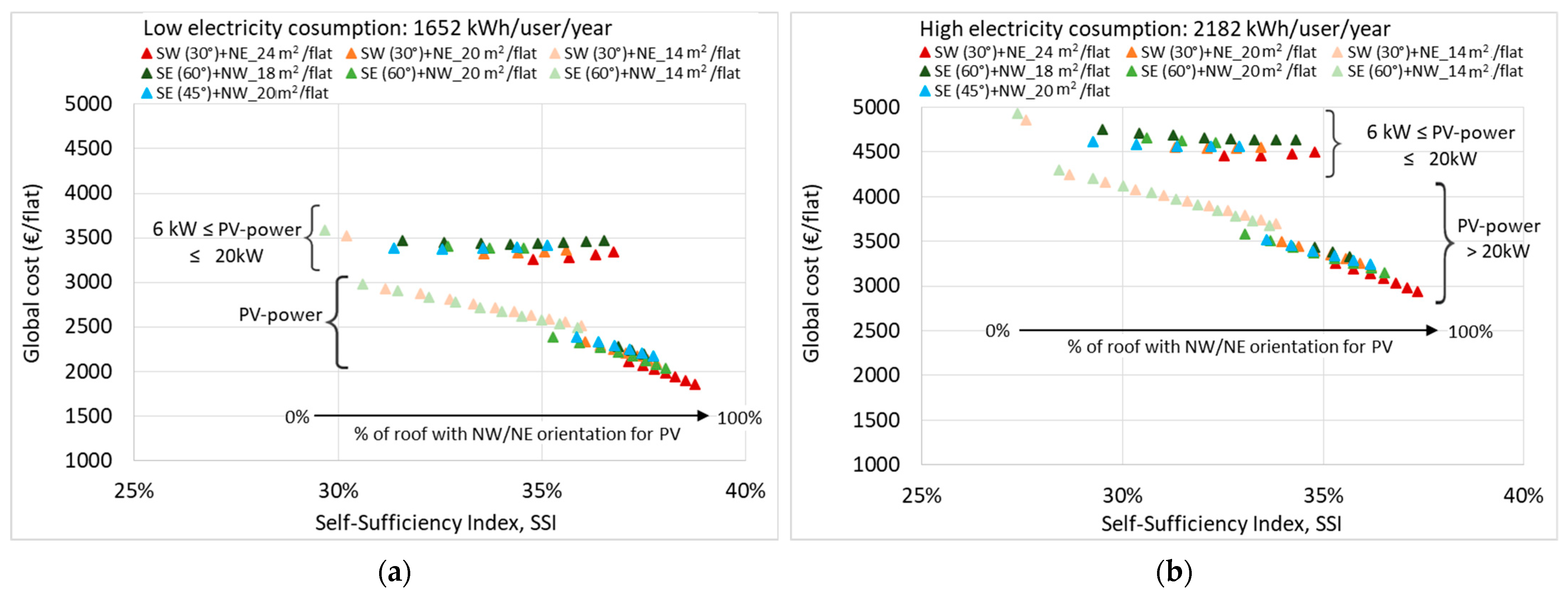
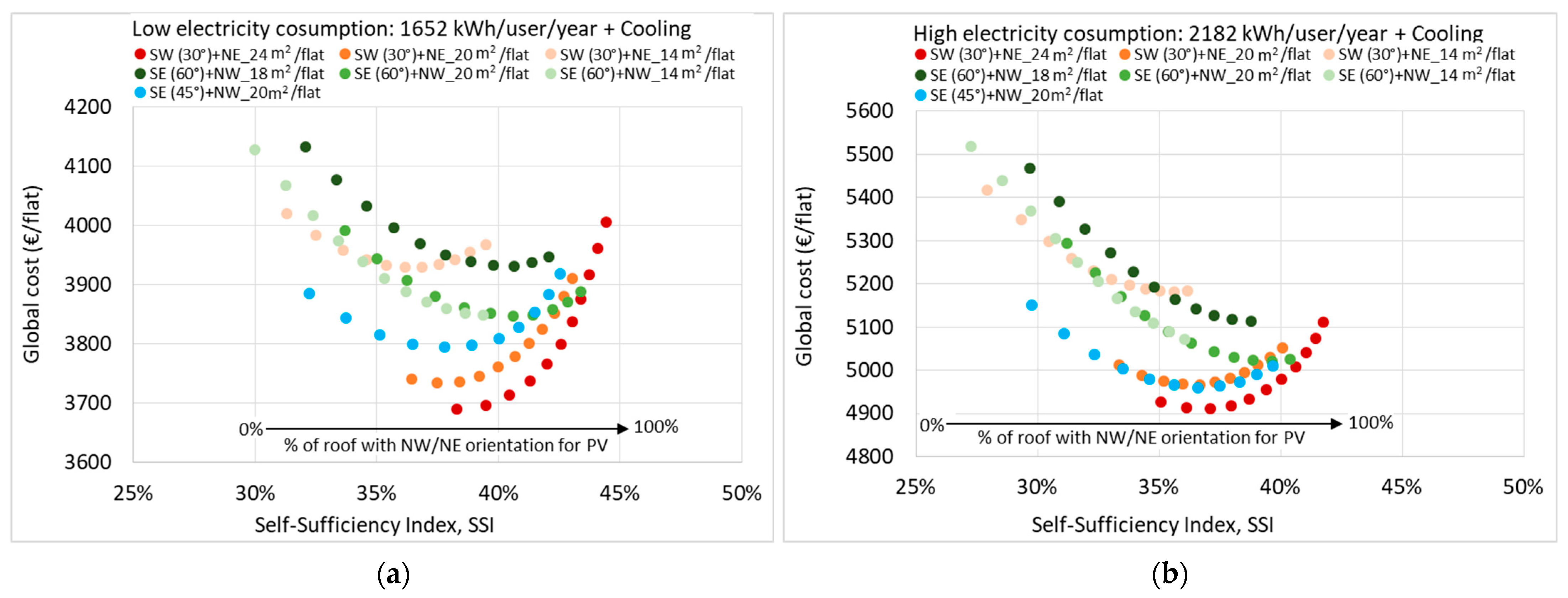
• Slightly higher SSI values are achieved for low-level consumers (1652 kWh/user/year), with a lower global cost than for high-level consumers. Small condominiums reach the highest levels of energy self-sufficiency, and the maximum SSI is 39% for a P equal to 22 kW for the well-oriented building (SW +30°, ID30). Moreover, the quota of PV per flat affects the energy self-sufficiency; the higher the quota of PV expressed as m²/flat is, the more SSI increases.
• It is always convenient to install PV for large condominiums, and when using 100% of the North-facing roof surface, a maximum SSI of 34–36% is achieved for a P of 38–40 kW.
• The global cost per flat varies from 3600 to 1850 €/flat for low electricity consumption and from 4900 to 2900 €/flat for high electricity consumption.

Similar trends to those described in Figure 11 can be observed when taking into account the total electricity consumption (S3 and S4). It has emerged, from Figure 12, that the global costs are higher whenever space cooling is considered, and the cost of energy in fact increases, but higher SSI values can also be achieved in this scenario.

In summary, these results show that the better the orientation is, the higher the energy self-sufficiency and the lower the energy costs and those for the installation of photovoltaic technologies.

Table 5. Energy and economic analysis using one and two rooftop PV orientations according to scenarios S3 and S4 (see Figure 12).

User	Building ID	100% South-Area and 0% North-Area				100% South-Area and 100% North-Area				Δ
		SCI (%)	SSI (%)	P (kW)	Global Cost (€/flat)	SCI (%)	SSI (%)	P (kW)	Global Cost (€/flat)	SSI (%)
Low-consumer	30	57	32	11	4133	44	42	22	2608	10
	91	51	34	16	3991	40	43	30	2386	9
	211	66	30	20	4129	51	39	38	2809	9
	140	53	38	15	3690	34	44	30	2192	6
	258	58	36	16	3740	40	43	30	2422	7
	199	75	31	19	4021	50	39	40	2870	8
	153	57	32	13	3885	70	43	29	2457	11
High-consumer	30	66	30	11	5468	51	39	22	3774	9
	91	60	31	16	5294	47	40	30	3523	9
	211	76	27	20	5520	59	36	38	4032	9
	140	61	35	15	4927	41	42	30	3298	7
	258	68	33	16	5012	47	40	30	3563	7
	199	85	28	19	5416	58	36	40	4085	8
	153	66	30	13	5151	47	40	29	3550	10

summarizes the main results obtained from the energy and economic analysis using one and two PV orientations according to scenarios S3 and S4. Small condominiums reach higher values of SSI, but have lower values of SCI than large condominiums. The costs for PV installation are lower if two rooftop orientations are used instead of one, thanks to the quota of installed P (1600 €/kW_p for 6 kW ≤ P ≤ 20 kW and 1000 €/kW_p for P > 20 kW). It can be concluded that SSI on average increases by 8.5% for the use of two PV orientations (100% of the south-area and 100% of the north-area).

A last future scenario was investigated assuming a constant lower cost for the PV technologies equal to 1600 €/kWp (independently by the PV power installed). Figure 13 and Figure 14 show the results for the cost-optimal analysis of the scenarios: S1, S2, S3 and S4. It can be seen that the more buildings have a high consumption, the more convenient it is to use two rooftop orientations for the PV installation.

In Figure 13 (as Figure 11), the global cost only refers to the energy consumption for light, appliances and condominium utilities. As previous emerged, the global cost for low-level consumers is lower than for high-level consumers and the orientation affects the convenience of the use of two orientations to a great extent. In fact, it is not always convenient to use the entire north-facing roof, especially for well-oriented buildings (SW 30°). The percentage of the north-facing roof that is convenient to use varies according to the shape of the building (e.g., PV surface/number of flats).

The results of the cost-optimal analysis, considering the energy consumption for space cooling (S3 and S4) are presented in Figure 14. Again, in this case, the results depend on the buildings orientation:

• It is almost always convenient to also use the North surfaces for buildings with a SE-NW oriented roof (more convenient for high-level consumers).
• It is almost never convenient to use the North surfaces for buildings with a SW-NE oriented roof (always a little more convenient for high-level consumers).
• With this GIS-based methodology it is possible to perform cost-benefit analyses on an urban scale but considering the specific characteristics of each single building (as for the building represented in light blue with a singular rooftop orientation).

Taken together, these results provide important insights into the investigation of costs and self-sufficiency of roof-integrated PV technologies on residential buildings using multiple orientations.

5. Discussion

Nowadays, many improvements are being made to the energy efficiency of household appliances, and thanks to the introduction of energy classes, electricity consumption has partially decreased. However, it is now necessary to exploit the renewable energy sources that are available locally.

In this work, a cost-optimal analysis was conducted to compare the economic implications of the different power levels of PVs installed on rooftops using all their orientations: south-facing and north-facing. The optimal level of self-sufficiency was identified as a function of the costs of the PV power installed and of the energy.

The results of this investigation, which took into account a real urban environment, show that it could be convenient to exploit all the potential rooftop surfaces with PV panels in high-density cities to considerably improve energy self-sufficiency, as well as to provide significant economic benefits for the residential users. These findings could contribute to our understanding to identify the optimum solution for PV systems installation. They may also provide a basis for the establishment of collective self-consumers and energy communities in urban environments.

One key finding of this work is that the shape of the building and the roof orientation influence the availability of solar energy and the energy performance of buildings. However, not only does the shape of the building significantly affect the availability of solar energy in urban environments, the urban morphology also does [43,44,45,46,47,48]. The identification of the optimal urban context with a high solar energy production, a high energy performance and a high energy security will be an important issue for future research. Local climate conditions also affect the production and consumption of PV energy [49,50], and this will also be further evaluated. In this work, a city in the North-West of Italy was used as a case study, but it would be interesting to evaluate how the benefits, in terms of costs and energy performance, vary for cities located in southern Italy, with its warmer climate with greater solar radiation intensity.

In a previous work [18], the authors promoted SCI and SSI at building and district levels using the integration of solar energy with PV-battery systems. From that analysis, it emerged that it is possible to achieve a higher level of the SCI and the SSI at the district scale by combining multiple condominiums at a city level. In future investigations, we will investigate different storage system scenarios in order to reduce the PV-battery size using roof surfaces with multiple orientations to improve not only the SSI but also the SCI. In addition, this type of methodology will also be applied at a district scale for two main reasons: (i) the economic incentives for the configuration of a renewable energy community are greater than for the collective self-consumer; (ii) the promotion of PV technologies for a group of buildings can improve energy self-sufficiency at a city level and not just at the building scale. In this study, residential users were analyzed, whereas further evaluations will also be performed considering different typologies of user profiles (e.g., municipal sector, offices, and schools). Another investigation could involve evaluating the energy and economic benefits of the combined installation of PV and solar thermal technologies [51].

The results of this work refer to the systems losses value of 14%. Since technologies are constantly evolving, would be interesting to evaluate the impact of other technologies such as high-efficient inverters. A preliminary analysis was performed considering an efficiency of 12 and 10% rather than 14%.

Table 6. Comparison of annual PV energy production data considering three energy losses scenarios (i.e., 14, 12 and 10%) for different rooftop orientations.

Azimuth (°)	Annual PV Production (kWh/kWp)
	14% of Energy Losses	12% of Energy Losses	10% of Energy Losses
SE = −60	1069	1094	1119
SE = −45	1098	1124	1149
SW = +30	1078	1103	1128
NW = +120	821	840	859
NW = +135	780	798	816
NE = −150	791	809	828

shows the annual PV energy production with the three energy losses scenarios (i.e., 14, 12, and 10%) for different rooftop orientations. Independently by rooftop orientations, com-pared to the 14% loss scenario, the energy production increases by 2.3–2.4% with the 12% scenario, and by 4.6–4.7% with 10% one. While, for each scenario, there is a significant difference between the PV energy production on rooftop with different orientations (the energy production can increase up to 41%). This impact on costs and energy self-sufficiency will be analyzed in more detail in future work.

Finally, in this work, the PV potential has been evaluated using data elaborated from the PVGIS portal, since the processing is fast and simple. However, from the analysis of the existing methods and tools used to evaluate the PV potential (see Section 2.1), it has emerged that GIS-based methodology tools allow much more accurate investigations to be performed with respect to using only the PVGIS portal. The complexity of GIS tools lies in the processing times of the input and output data and in the simulation times. The analyses carried out with GIS tools are more accurate because the real urban environment is taken into account, thanks to the use of DSMs (e.g., the presence of disturbing elements). The description of the context is important to obtain reliable results, as the more accurate the input data are (e.g., the precision of the DSM), the better the outputs are able to return real data.

6. Conclusions

Solar energy is often the only renewable source available in cities, and therefore to promote self-consumption and energy self-sufficiency, it is necessary to exploit all the potential PV areas on rooftops. In the city of Turin, as in general occurs in the European context, it is common to use only the South-exposed surfaces of roofs. This research has focused on whether it is possible to use multiple orientations for the production of electricity and reap both energy and economic benefits.

The aim of the present research has been to examine the energy and economic benefits of roof integrated PV technologies considering two orientations. The analysis was performed on seven residential buildings located in a neighborhood in the city of Turin, Italy. These buildings are condominiums with different dimensions, orientations and consumptions, while their roof slopes vary from 23 to 27°. The PV potential was identified for each building through the use of GIS tools and information taken from the PVGIS portal. The hourly load profile was analyzed by quantifying the electricity for light and appliances considering low-level and high-level residential consumers, the electricity for space cooling using a GIS-based engineering model, and the electricity for condominium utilities. The SCI and SSI indexes were assessed at a building level for a typical meteorological year, while evaluating different scenarios.

The results of this investigation show that the dimensions, the types of consumer and the orientations of buildings affect energy self-sufficiency. In general, without using storage systems, as the SCI increases, the SSI decreases more or less quickly as a function of the building typology. When considering the use of two roof orientations, the maximum level of achieved SSI was on average 41.8, 41.5 and 35.7% for small, medium and large condominiums, respectively. The economic benefits were investigated by applying a cost-optimal analysis, which showed that, for the investigated building stock and considering the use of two PV systems orientations, the SSI increased on average by 8.5%, with additional economic benefits for the cost of energy and the cost for the PV installation. The findings in this study provide a new understanding of how to exploit the solar energy potential in order to improve the energy performance of buildings, increase energy security and reduce energy costs.

In future works this methodology will be implemented taking into account storage systems and using GIS tools for the PV potential analysis. Furthermore, the methodology will be applied to a larger sample of buildings, to evaluate different types of consumers, producers and prosumers at a neighborhood scale. Different economic incentives will be considered, for collective self-consumer and renewable energy community configurations. Incentive policies can have a very important impact on the costs of the technologies that can increase due to the high request; therefore, this methodology can also evaluate the economic impact of future incentive policies that can be quite different from the one hypothesized in this work.

Finally, since the urban context affects electricity consumption and the potential solar energy, different urban morphologies will be analyzed in various cities and climates.

References

1. Benasla, M.; Hess, D.; Allaoui, T.; Brahami, M.; Denaï, M. The transition towards a sustainable energy system in Europe: What role can North Africa’s solar resources play? Energy Strateg. Rev. 2019, 24, 1–13. [Google Scholar] [CrossRef]
2. Collier, M.J.; Nedović-Budić, Z.; Aerts, J.; Connop, S.; Foley, D.; Foley, K.; Newport, D.; McQuaid, S.; Slaev, A.; Verburg, P. Transitioning to resilience and sustainability in urban communities. Cities 2013, 32, S21–S28. [Google Scholar] [CrossRef] [Green Version]
3. Gielen, D.; Boshell, F.; Saygin, D.; Bazilian, M.D.; Wagner, N.; Gorini, R. The role of renewable energy in the global energy transformation. Energy Strateg. Rev. 2019, 24, 38–50. [Google Scholar] [CrossRef]
4. Delponte, I.; Schenone, C. RES Implementation in Urban Areas: An Updated Overview. Sustainability 2020, 12, 382. [Google Scholar] [CrossRef] [Green Version]
5. Defaix, P.R.; van Sark, W.G.J.H.M.; Worrell, E.; de Visser, E. Technical potential for photovoltaics on buildings in the EU-27. Sol. Energy 2012, 86, 2644–2653. [Google Scholar] [CrossRef] [Green Version]
6. Tröndle, T.; Pfenninger, S.; Lilliestam, J. Home-made or imported: On the possibility for renewable electricity autarky on all scales in Europe. Energy Strateg. Rev. 2019, 26, 100388. [Google Scholar] [CrossRef]
7. Boulahia, M.; Djiar, K.A.; Amado, M. Combined Engineering—Statistical Method for Assessing Solar Photovoltaic Potential on Residential Rooftops: Case of Laghouat in Central Southern Algeria. Energies 2021, 14, 1626. [Google Scholar] [CrossRef]
8. Thebault, M.; Clivillé, V.; Berrah, L.; Desthieux, G. Multicriteria roof sorting for the integration of photovoltaic systems in urban environments. Sustain. Cities Soc. 2020, 60, 102259. [Google Scholar] [CrossRef]
9. Khan, J.; Arsalan, M.H. Estimation of rooftop solar photovoltaic potential using geo-spatial techniques: A perspective from planned neighborhood of Karachi—Pakistan. Renew. Energy 2016, 90, 188–203. [Google Scholar] [CrossRef]
10. Wong, M.S.; Zhu, R.; Liu, Z.; Lu, L.; Peng, J.; Tang, Z.; Lo, C.H.; Chan, W.K. Estimation of Hong Kong’s solar energy potential using GIS and remote sensing technologies. Renew. Energy 2016, 99, 325–335. [Google Scholar] [CrossRef]
11. Ruiz, H.S.; Sunarso, A.; Ibrahim-Bathis, K.; Murti, S.A.; Budiarto, I. GIS-AHP Multi Criteria Decision Analysis for the optimal location of solar energy plants at Indonesia. Energy Rep. 2020, 6, 3249–3263. [Google Scholar] [CrossRef]
12. Firozjaei, M.K.; Nematollahi, O.; Mijani, N.; Shorabeh, S.N.; Firozjaei, H.K.; Toomanian, A. An integrated GIS-based Ordered Weighted Averaging analysis for solar energy evaluation in Iran: Current conditions and future planning. Renew. Energy 2019, 136, 1130–1146. [Google Scholar] [CrossRef]
13. Mansouri Kouhestani, F.; Byrne, J.; Johnson, D.; Spencer, L.; Hazendonk, P.; Brown, B. Evaluating solar energy technical and economic potential on rooftops in an urban setting: The city of Lethbridge, Canada. Int. J. Energy Environ. Eng. 2019, 10, 13–32. [Google Scholar] [CrossRef] [Green Version]
14. Bódis, K.; Kougias, I.; Jäger-Waldau, A.; Taylor, N.; Szabó, S. A high-resolution geospatial assessment of the rooftop solar photovoltaic potential in the European Union. Renew. Sustain. Energy Rev. 2019, 114, 109309. [Google Scholar] [CrossRef]
15. Pontes Luz, G.; e Silva, R. Modeling Energy Communities with Collective Photovoltaic Self-Consumption: Synergies between a Small City and a Winery in Portugal. Energies 2021, 14, 323. [Google Scholar] [CrossRef]
16. Mutani, G.; Santantonio, S.; Beltramino, S. Indicators and Representation Tools to Measure the Technical-Economic Feasibility of a Renewable Energy Community. The Case Study of Villar Pellice (Italy). Int. J. Sustain. Dev. Plan. 2021, 16, 1–11. [Google Scholar] [CrossRef]
17. Ciocia, A.; Amato, A.; Di Leo, P.; Fichera, S.; Malgaroli, G.; Spertino, F.; Tzanova, S. Self-Consumption and Self-Sufficiency in Photovoltaic Systems: Effect of Grid Limitation and Storage Installation. Energies 2021, 14, 1591. [Google Scholar] [CrossRef]
18. Todeschi, V.; Marocco, P.; Mutani, G.; Lanzini, A.; Santarelli, M. Towards Energy Self-consumption and Self-sufficiency in Urban Energy Communities. Int. J. Heat Technol. 2021, 39, 1–11. [Google Scholar] [CrossRef]
19. Gómez-Navarro, T.; Brazzini, T.; Alfonso-Solar, D.; Vargas-Salgado, C. Analysis of the potential for PV rooftop prosumer production: Technical, economic and environmental assessment for the city of Valencia (Spain). Renew. Energy 2021, 174, 372–381. [Google Scholar] [CrossRef]
20. Gagnon, P.; Margolis, R.; Melius, J.; Phillips, C.; Elmore, R. Estimating rooftop solar technical potential across the US using a combination of GIS-based methods, lidar data, and statistical modeling. Environ. Res. Lett. 2018, 13, 24027. [Google Scholar] [CrossRef]
21. Singh, D.; Gautam, A.K.; Chaudhary, R. Potential and performance estimation of free-standing and building integrated photovoltaic technologies for different climatic zones of India. Energy Built Environ. 2020. [Google Scholar] [CrossRef]
22. Yang, Y.; Campana, P.E.; Stridh, B.; Yan, J. Potential analysis of roof-mounted solar photovoltaics in Sweden. Appl. Energy 2020, 279, 115786. [Google Scholar] [CrossRef]
23. Oh, M.; Kim, J.-Y.; Kim, B.; Yun, C.-Y.; Kim, C.K.; Kang, Y.-H.; Kim, H.-G. Tolerance angle concept and formula for practical optimal orientation of photovoltaic panels. Renew. Energy 2021, 167, 384–394. [Google Scholar] [CrossRef]
24. Hartner, M.; Ortner, A.; Hiesl, A.; Haas, R. East to west—The optimal tilt angle and orientation of photovoltaic panels from an electricity system perspective. Appl. Energy 2015, 160, 94–107. [Google Scholar] [CrossRef]
25. Azaioud, H.; Desmet, J.; Vandevelde, L. Benefit Evaluation of PV Orientation for Individual Residential Consumers. Energies 2020, 13, 5122. [Google Scholar] [CrossRef]
26. Mubarak, R.; Weide Luiz, E.; Seckmeyer, G. Why PV Modules Should Preferably No Longer Be Oriented to the South in the Near Future. Energies 2019, 12, 4528. [Google Scholar] [CrossRef] [Green Version]
27. Lahnaoui, A.; Stenzel, P.; Linssen, J. Tilt Angle and Orientation Impact on the Techno-economic Performance of Photovoltaic Battery Systems. Energy Procedia 2017, 105, 4312–4320. [Google Scholar] [CrossRef]
28. Mainzer, K.; Fath, K.; McKenna, R.; Stengel, J.; Fichtner, W.; Schultmann, F. A high-resolution determination of the technical potential for residential-roof-mounted photovoltaic systems in Germany. Sol. Energy 2014, 105, 715–731. [Google Scholar] [CrossRef]
29. Ng, K.M.; Adam, N.M.; Inayatullah, O.; Kadir, M.Z.A.A. Assessment of solar radiation on diversely oriented surfaces and optimum tilts for solar absorbers in Malaysian tropical latitude. Int. J. Energy Environ. Eng. 2014, 5, 75. [Google Scholar] [CrossRef] [Green Version]
30. Hong, T.; Lee, M.; Koo, C.; Jeong, K.; Kim, J. Development of a method for estimating the rooftop solar photovoltaic (PV) potential by analyzing the available rooftop area using Hillshade analysis. Appl. Energy 2017, 194, 320–332. [Google Scholar] [CrossRef]
31. Suomalainen, K.; Wang, V.; Sharp, B. Rooftop solar potential based on LiDAR data: Bottom-up assessment at neighbourhood level. Renew. Energy 2017, 111, 463–475. [Google Scholar] [CrossRef]
32. Todeschi, V.; Mutani, G.; Baima, L.; Nigra, M.; Robiglio, M. Smart Solutions for Sustainable Cities—The Re-Coding Experience for Harnessing the Potential of Urban Rooftops. Appl. Sci. 2020, 10, 7112. [Google Scholar] [CrossRef]
33. Zheng, Y.; Weng, Q.; Zheng, Y. A hybrid approach for three-dimensional building reconstruction in indianapolis from LiDAR data. Remote Sens. 2017, 9, 310. [Google Scholar] [CrossRef] [Green Version]
34. Gracia-Amillo, A.M.; Bardizza, G.; Salis, E.; Huld, T.; Dunlop, E.D. Energy-based metric for analysis of organic PV devices in comparison with conventional industrial technologies. Renew. Sustain. Energy Rev. 2018, 93, 76–89. [Google Scholar] [CrossRef]
35. Mutani, G.; Santantonio, S.; Brunetta, G.; Caldarice, O.; Demichela, M. An energy community for territorial resilience: Measurement of the risk of an energy supply blackout. Energy Build. 2021, 240, 110906. [Google Scholar] [CrossRef]
36. Mutani, G.; Todeschi, V.; Beltramino, S. Energy Consumption Models at Urban Scale to Measure Energy Resilience. Sustainability 2020, 12, 5678. [Google Scholar] [CrossRef]
37. Mutani, G.; Todeschi, V.; Santantonio, S. Urban-Scale Energy Models: The relationship between cooling energy demand and urban form. In Proceedings of the 38th UIT Heat Transfer Conference, Padua, Italy, 21–23 June 2021. [Google Scholar]
38. Walter, E.; Kämpf, J.H. A verification of CitySim results using the BESTEST and monitored consumption values. In Proceedings of the 2nd Building Simulation Applications BSA 2015, Bozen-Bolzano, Italy, 4–6 February 2015; pp. 215–222. [Google Scholar]
39. De Almeida, A.; Hirzel, S.; Patrão, C.; Fong, J.; Dütschke, E. Energy-efficient elevators and escalators in Europe: An analysis of energy efficiency potentials and policy measures. Energy Build. 2012, 47, 151–158. [Google Scholar] [CrossRef]
40. Tukia, T.; Uimonen, S.; Siikonen, M.-L.; Donghi, C.; Lehtonen, M. High-resolution modeling of elevator power consumption. J. Build. Eng. 2018, 18, 210–219. [Google Scholar] [CrossRef] [Green Version]
41. Tukia, T.; Uimonen, S.; Siikonen, M.-L.; Hakala, H.; Donghi, C.; Lehtonen, M. Explicit method to predict annual elevator energy consumption in recurring passenger traffic conditions. J. Build. Eng. 2016, 8, 179–188. [Google Scholar] [CrossRef] [Green Version]
42. Tukia, T.; Uimonen, S.; Siikonen, M.-L.; Donghi, C.; Lehtonen, M. Modeling the aggregated power consumption of elevators—The New York city case study. Appl. Energy 2019, 251, 113356. [Google Scholar] [CrossRef]
43. Mutani, G.; Todeschi, V.; Carozza, M.; Rolando, A. Urban-Scale Energy Models: Relationship between urban form and energy performance. In Proceedings of the 2020 IEEE 3rd International Conference and Workshop in Óbuda on Electrical and Power Engineering (CANDO-EPE), Budapest, Hungary, 18–19 November 2020; pp. 185–190. [Google Scholar]
44. Sanaieian, H.; Tenpierik, M.; van den Linden, K.; Mehdizadeh Seraj, F.; Mofidi Shemrani, S.M. Review of the impact of urban block form on thermal performance, solar access and ventilation. Renew. Sustain. Energy Rev. 2014, 38, 551–560. [Google Scholar] [CrossRef]
45. Vartholomaios, A. The residential solar block envelope: A method for enabling the development of compact urban blocks with high passive solar potential. Energy Build. 2015, 99, 303–312. [Google Scholar] [CrossRef]
46. De Lemos Martins, T.A.; Adolphe, L.; Bastos, L.E.; de Lemos Martins, M.A. Sensitivity analysis of urban morphology factors regarding solar energy potential of buildings in a Brazilian tropical context. Sol. Energy 2016, 137, 11–24. [Google Scholar] [CrossRef]
47. van Esch, M.M.E.; Looman, R.H.J.; de Bruin-Hordijk, G.J. The effects of urban and building design parameters on solar access to the urban canyon and the potential for direct passive solar heating strategies. Energy Build. 2012, 47, 189–200. [Google Scholar] [CrossRef]
48. Machete, R.; Falcão, A.P.; Gomes, M.G.; Moret Rodrigues, A. The use of 3D GIS to analyse the influence of urban context on buildings’ solar energy potential. Energy Build. 2018, 177, 290–302. [Google Scholar] [CrossRef]
49. Beccali, M.; Bonomolo, M.; Di Pietra, B.; Leone, G.; Martorana, F. Solar and Heat Pump Systems for Domestic Hot Water Production on a Small Island: The Case Study of Lampedusa. Appl. Sci. 2020, 10, 5968. [Google Scholar] [CrossRef]
50. Staffell, I.; Pfenninger, S. The increasing impact of weather on electricity supply and demand. Energy 2018, 145, 65–78. [Google Scholar] [CrossRef]
51. Ul Abdin, Z.; Rachid, A. A Survey on Applications of Hybrid PV/T Panels. Energies 2021, 14, 1205. [Google Scholar] [CrossRef]
Figure 1. Annual solar radiation (kWh/m2/year) (a) using a DSM of 5 m and annual local climatic data; (b) using a DSM with a precision of 0.5 m and monthly local climatic data.
Energies 14 04018 g001
Figure 2. Monthly horizontal irradiation values (kWh/m2/year) on the rooftop of the buildings at block of buildings scale using different input data, types of simulation and tools: ArcGIS, PVGIS and measured data from a weather station. On the right the number of simulations, the simulation times, and the annual mean absolute percentage error (MAPE) for each analysis have been indicated.
Energies 14 04018 g002
Figure 3. Comparison of the monthly solar radiation values (kWh/m2/year) considering four orientations: (a) SE (azimuth −60°, (b) SW (azimuth +30°), (c) NW (azimuth +120°), (d) and NE (azimuth −150°).
Energies 14 04018 g003
Figure 4. Distribution of the annual electrical consumption of 107 residential users for the year 2016.
Energies 14 04018 g004
Figure 5. Comparison of the hourly cooling demands for the five typical summer days simulated with the GIS-based model (in red), the CitySim tool (in green) and the hourly method according to ISO 52016 (in blue), on the secondary axis the solar radiation expressed in Wh/m2 is indicated (in yellow): (a) a residential building built in 1961–1970 with SW (azimuth +30°) orientation; (b) a residential building built in 1919–1945 with SE (azimuth −60°) orientation.
Energies 14 04018 g005
Figure 6. The influence of outdoor air temperature on daily energy demand for space cooling for: (a) residential building built in 1961–1970 with SW (azimuth +30°) orientation; (b) residential building built in 1919–1945 with SE (azimuth −60°) orientation.
Energies 14 04018 g006
Figure 7. Typical hourly profile of elevator in residential buildings [42].
Energies 14 04018 g007
Figure 8. Orientation of the buildings in the city of Turin.
Energies 14 04018 g008
Figure 9. Hourly profiles of the load and PV production for 12 typical days, each of which is representative of a specific month of the year 2016: (a) small condominium with SE −60° orientation, (b) medium condominium with SE −60° orientation, (c) large condominium with SE −60° orientation, (d) small condominium with SW +30° orientation, (e) medium condominium with SW +30° orientation, (f) large condominium with SW +30° orientation, (g) medium condominium with SE −45° orientation.
Energies 14 04018 g009aEnergies 14 04018 g009b
Figure 10. Analysis of SCI and SSI for condominiums with different dimensions and orientations distinguishing between (a) low-level consumers with an electricity consumption of 1652 kWh/user/year and (b) and high-level consumers with an electricity consumption of 2182 kWh/user/year.
Energies 14 04018 g010
Figure 11. Global-cost analysis for residential users: SSI as a function of the global cost per flat considering different levels of installed PV power and energy consumption for (a) low-level consumers (S1) and (b) high-level consumers (S2).
Energies 14 04018 g011
Figure 12. Global-cost analysis for residential users: SSI as a function of the global cost per flat considering different levels of installed PV power and energy consumption for (a) low-level consumers (S3) and (b) high-level consumers (S4).
Energies 14 04018 g012
Figure 13. Global-cost analysis for residential users: SSI as a function of the global cost per flat considering different levels of installed PV power and energy consumption for (a) low-level consumers (S1) and (b) high-level consumers (S2).
Energies 14 04018 g013
Figure 14. Global-cost analysis for residential users: SSI as a function of the global cost per flat considering different levels of installed PV power and energy consumption for (a) low-level consumers (S3) and (b) high-level consumers (S4).
Energies 14 04018 g014