A TensorFlow Approach to Data Analysis for Time Series Forecasting in the Energy-Efficiency Realm

Abstract

Thanks to advances in smart metering devices (SM), the electricity sector is undergoing a series of changes, among which it is worth highlighting the ability to control the response to all events that occur in the electricity grid with the intention of making it more smart. Predicting electricity consumption data is a key factor for the energy sector in order to create a completely intelligent electricity grid that optimizes consumption and forecasts future energy needs. However, it is currently not enough to give a prediction of energy consumption (EC), but it is also necessary to give the prediction as fast as possible so that the grid can operate in the shortest possible time. An approach for developing EC prediction systems is introduced here by the use of artificial neural networks (ANN). Differently from other research studies on the subject, a divide-and-conquer strategy is used so that the target system’s execution switches from one to another specialized small models that forecast the EC of a building within the time range of one hour. By simultaneously processing a large amount of data and models, a consequence of implementing them in parallel with TensorFlow on GPUs, the training procedure proposed here increases the performance of the classic time series prediction methods, which are based on ANN. Leveraging the latest generation of ANN techniques and new GPU-based architectures, correct EC predictions can be obtained and, as the experimentation carried out in this work shows, such predictions can be obtained quickly. The obtained results in this study show a promising way for speeding up big data processing of building’s monitoring data to achieve energy efficiency.

1. Introduction

Energy consumption (EC) is rocketing globally as developing countries catch up with the developed ones, and thereby there is a higher emission of polluting gases into the atmosphere than ever before. This effect will be worsened as the world’s population grows and technology development becomes greater in modern society. In particular, the EC in buildings represents approximately 40% of the world’s energy consumption and currently represents a significant part of the global energy market [1]. This is why EC prediction has become one of the most critical fields of research to achieve energy efficiency in the building sector [2], and thus it is gaining increasing importance among the world’s strategic issues pending of resolution due to the growing cost of energy as well as the environmental impact that is a consequence of such an enormous share of energy consumption.

There is an enormous increase in data from buildings [3] that can be processed in real time thanks to the recent development of new sensing technologies with massive collection and storage of these data. This fact allows us to constantly monitor buildings [4], which must now be timely treated and analyzed to make useful predictions on energy consumption. Therefore, it becomes of paramount importance to have an effective strategy that allows us to quickly make decisions regarding achieving savings in EC from large sets of monitored data from buildings that are obtained subject to time-critical conditions [5].

According to [6], to obtain EC predictions for buildings in real time, it is necessary to have the support of parallelization methods based on modern multi- and many-core programming [7], especially, those based on GPU architectures for high performance computing (HPC) [8,9]. Moreover, today state-of-art methodologies and technologies for EC prediction in buildings may become quickly obsolete in the next few years so there is a need to explore different alternatives. This situation not only directs the researcher to consider which precise technique must be used to solve a particular problem, but also to evaluate the most suitable HPC deployment, which is necessary so that the software being developed can cope with the immense volume of data generated by sensing instruments currently installed in buildings [10]. The latter scenario will persist in the years to come.

Based on the current scientific literature on the subject, some research can be found on ways to improve energy efficiency (EE) in buildings [11,12]. However, in several of these recent papers the authors propose data processing methodologies that are based solely on sequential algorithms, i.e., they do not consider any specific treatment for the processing of big data [13] nor deploy any method to obtain an optimal prediction model based on the time-series of EC data in buildings. These methodologies also do not use strategies to reduce the training time of the models they implement, for example, by mostly using k-fold cross validation methods, as defined in [14], that serve to determine a stop criterion for the iterations of the algorithm. Moreover, no data with time-constrained restrictions are treated in the latter mentioned article, as is done in the study referred to in [15]. In the last work, a solution is proposed for a posteriori understanding of EC patterns. Therefore, to respond to the aspects related to the aforementioned issues (treatment of big data, predictions based on time series, temporal restrictions, and use of parallelism to accelerate training), this paper proposes an innovative methodology in order to obtain optimal solutions to be able to make time-critical predictions of EC in buildings.

There are recent contributions in the research line that we pursue [16,17], which can be classified in four groups (a–d) as follows: (a) Energy predictions based on classical (non-parallelized) methods for training and executing artificial neural networks (ANN) of which one of the most representative works is by Beccali et al. [18], which carries out an energy auditing in public buildings in the south of Italy. In that work, they created and implemented an energy database which was used to deploy an ANN-based tool for decision making. A deep neural network is used in [14] for energy demand forecasting in buildings that shows accurate and robust predictions. In [19], ANN are used for sun energy forecasting in order to guarantee reliable electricity supply and reduce pollution by means of prediction algorithms and pattern similarities. (b) EC forecasting by processing the time-series of big data (BD), e.g., the study presented by Pérez et al. [15], shows advanced parallelization techniques for obtaining EC patterns that solve the problem of prediction. In the latter case, parallelized versions of voting-based clustering algorithms are used so as to assign the optimal number of each cluster. For a detailed survey of big data clustering techniques, we have to mention the relevant paper of [20]. (c) EC predictions based on the optimization of a model as it is shown in [21]. In prior studies, we can observe how a non-parallelized first approach to the problem is performed in [22], where the parameters of networks are adjusted by trial and error to obtain the models that produce the best results. Furthermore, a sequential evolutionary algorithm is developed in [23] to optimize the weights of neural networks that minimize prediction errors efficiently. In [24], the authors propose to use a weighted support vector regression model combined with a differential evolution technique as the basis of an optimization algorithm for electric power load forecasting of an institutional building at the University of Singapore. (d) Parallel architectures for time-series forecasting of EC data in databases. Random Forest is one of the most used methods, mainly due to its easy implementation in distributed environments. In the article of [25], it was applied to massive data sets and showed a good performance. However, there are several studies that point out the convenience of optimizing the obtained errors with this technique. Thereby, the research carried out in [26] is considered as the solution for filling up this gap on the subject nowadays.

Backpropagation algorithms generally minimize the error function by using the direction with the most slope in the stochastic gradient descent method, which is regularly used in training networks; the problem with these algorithms is that they are often very inefficient and inaccurate due to the shape of the error hyper-surface. Other alternatives have been explored to speed up the long computation time needed to train neural networks, such as recurrent neural networks with feedback loops, which are capable of processing temporal patterns. Recurrent neural networks are an elegant way to increase the capacity of feed-forward neural networks to deal with complex models, but they also suffer from the original issue of neural networks in that the training phases are computationally time-consuming.

The intrinsic parallelism of neural network models has always been there, but it is only since the advent of cheap massively parallel GPU processors and graphics cards that it has become feasible to elegantly implement feed-forward neural networks to be able to process more complex datasets and problems such as those whose processed data are a time series.

In this work, we apply simple data parallelism to accelerate classical gradient descent-based algorithms for training neural networks and have achieved this by using TensorFlow, which does not require advanced knowledge of parallelism and the entire programming part of the training phase can be efficiently programmed using GPU hardware in a way that is almost transparent to the programmer.

Multi-pass predictions are made by formulating several sub-problems, which are independently solved according to a distributed framework. We have shown that by combining state-of-art ANN techniques, it is feasible to obtain accurate EC predictions made within strict time constraints. The approach combines techniques that are currently used for BD processing and proposes a new methodology for obtaining the foremost performance out of available resources to get the best possible predictions with time criticality.

The type of ANN here used to achieve the study’s objectives is the multilayer perceptron (MLP) [27]. Taking advantage of the parallel processing that modern GPUs currently offer us, we were able to achieve parallel execution of MLP networks [28]. Specifically, the work carried out here leverages the TensorFlow framework for this purpose in order to carry out a comparative study of two solutions to perform a fast prediction of the EC of buildings using ANN models.

Our proposal improves the accuracy of the solutions found so far by increasing the performance of the optimization method, thus allowing huge amounts of data and complex ANN-based models to be processed simultaneously. In order to achieve the objectives of our research, we approach the problem on the basis of two main points, i.e., by leveraging available high-performance computing resources to parallelize the training phase of the models as much as possible, and by dividing the initial problem into many small subproblems. The division into many subproblems is computationally efficient because they are quickly solved thanks to the high performance of GPUs on processing models that present data parallelism, such as that which can be extracted naturally from the aforementioned software applications, programmed using neural networks. The approach we have taken provides a system for processing massive time-critical data streams with, which is necessary for decision-making in real time, as noted in the results section of the paper. In addition, a comparative study of two different approaches is carried out to solve the problem of predicting energy consumption with time constraints. We can see in the study that a benefit is obtained by opting for a parallel approach with respect to a sequential proposal to solve the energy consumption prediction problem. The former not only manages to find a more accurate solution than the latter, but also obtains it in an incomparably less time than the solution based on a classical sequential EC prediction algorithm. In this way, the main objective of the present study is achieved, i.e., to provide a method to obtain optimal solutions produced within strict time constraints.

In this study, we have worked with EC data from buildings at the University of Granada (UGR). Due to the current power–metering system being relatively new, the amount of available data is not the same for all buildings. With respect to the EC data that we used in this study, it should be taken into account that the minimum time granularity was hours. The UGR facilities include classrooms, laboratories, and research centers. The UGR is composed of five campuses: Center, Cartuja, Fuentenueva, Aynadamar, and PTS. In total, they constitute 25 colleges distributed throughout the campus.

We propose an efficient implementation of the training phase for ANN models with GPU hardware, generating efficient PTX code for the latest generation of NVIDIA graphic cards by using the TensorFlow platform, which is easy to program even for developers with basic knowledge of parallelism. The proposed model allows one to obtain 24 different trained neuron network models (one per hour of energy consumption to predict) in the time that a single one would, implemented with a sequential algorithm, and in a much shorter time than a conventional model would train a single model (as shown by the experimentation carried out), taking advantage of the features and combining the benefits of parallelism and GPU cards in the execution of code. This fact is not currently widespread in the real applications currently carried out by researchers and our opinion is that it is totally innovative at this time. In this work, we provide an ample set of measurements, see, for example, Section 5.3 (Tables 1 and 2), which show 63% reductions in execution time when 24 models are sent to the GPU in batches while keeping 90% GPU computing power and 99% CPU usage, and a full usage of the global memory of the GPU card.

The rest of the article is divided as follows: Section 2 describes the ANN models developed here and their recent applications. Section 3 is centred on the technologies and existing GPU libraries to work with ANN. Section 4 introduces modeling of time series and energy efficiency. Section 5 puts forward the proposed models. Section 6 gathers the experimentation carried out and the obtained results. Finally, Section 7 presents the conclusions drawn from this research work and future studies.

2. Neural Networks

This study comprises several stages, the first one is dedicated to the data extraction phase, which is carried out automatically by an on- premises system of the UGR that is in charge of capturing and storing energy consumption (EC) raw data of each one of the buildings considered in this research work. Subsequently, the selection and pre-processing of data is carried out in the second stage, to finally be able to analyze and model the EC of buildings and, in this way, obtaining a prediction model of energy consumption in the third stage. By taking advantage of facilities that are currently offered by GPU processors, two ANN models are proposed, which are implemented in TensorFlow. Finally, a comparative study of the latter two is carried out to verify which is the best performance that can be obtained from each of the considered models.

In a very summarized way, we could say that the fundamental objective of this paper is to provide a method for EC forecasting through the use of ANN models, with the additional benefit of leveraging the high performance computing that would be obtained from data processing with GPUs to reduce the time cost in the training stage of each neural network implemented in the models.

Since there are previous publications in which the application of time series to solve the problem of EC prediction showed excellent results in several realms [18,29,30,31], the study presented here can be considered an advance in the prediction of EC in buildings, which is supported by our previous investigations that guarantees obtaining good results in terms of EC predictions, within a limited time span since the data are selected and read in the system. As part of the research work in the near future, we plan to leverage the prediction framework of our approach to be able to detect anomalous situations regarding energy consumption. The foundation of our proposal is that MLP is a widely deployed ANN model used worldwide for solving both classification [13,32] and prediction problems, as the latter applies to this study. For a deeper and detailed review of energy consumption models and energy efficiency tools, the reader is addressed to [33].

In Dudek’s work [34], a feedforward neural network was used to predict electricity cost, however, it is worth to mention that the input variables did not receive an appropriate pre-processing treatment as usually occurs in time series problems resolution methods.Probably because, Dudek did not carry out detrending, deseasonality or decomposition, but the input variables were not non-linearly processed to obtain the point to be predicted by the MLP. Azimi et al. 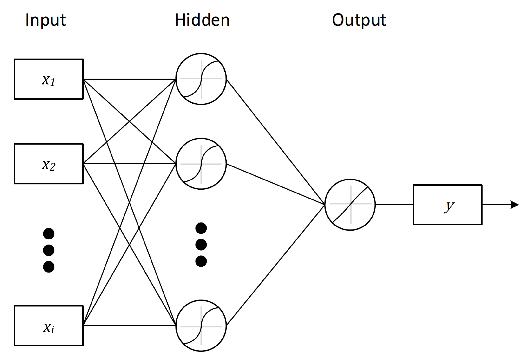[35] propose an interesting hybrid method made of clustering and MLP for predicting hourly solar radiation. The later paper proposes a solution similar to the one presented here to improve model’s prediction accuracy, i.e., the initial problem is divided into small sub-problems described by specialized models. The advantage of our approach consists of not only leveraging the division strategy for accuracy improvement, but also in being able to take advantage of the runtime optimization, which however the previous work did not take into account. The structure of a MLP neural network is depicted in Figure 1. This model is made up of one or more hidden layers, so that it intends to model an output $y_i$ from a given input $x_i$ of size k. In that way, a neural network is capable of modeling the output as the following Equation (1) denotes:

$$y_i=h(x_i^1,x_i^2,\dots ,x_i^k)+\epsilon$$

(1)

where $h\left(\right)$ is a non-linear function that depends on the k input data $x_i$, and $\epsilon$ is the error made by the network in estimating the value of the output $y_i$. According to Equation (2), an MLP is capable of modeling a time series $y\left(t\right)$ as the following equation shows:

$$y\left(t\right)=h\left(x\right(t-1),x(t-2),\dots ,x(t-p\left)\right)+\epsilon \left(t\right).$$

(2)

The input data of the MLP are the p past-values extracted from the time series and from them the next value $y\left(t\right)$ is predicted. In our case, the data will be transformed in such a way that the immediate p previous values need to be considered, i.e., the p hourly values before the hour t to be predicted. Therefore, the model uses the p previous hours as input x($t-1$), x($t-2$), …, x($t-p$) in the first layer, and then it predicts the consumption of the next hour $\left(y\right(t)=x(t)$), which is returned in the output layer.

The number of hidden layers and the amount of neurons are calculated by trial-and-error until a topology that yields the best possible performance is obtained. It is well known that a neural network with only one hidden layer must have the same modeling capability as one with several hidden layers [36]. Having this principle into account, only one hidden layer has been deployed in this research work to then calculate the optimal number of neurons located in that single layer. The more neurons in the hidden layer, the more complex the neural network is, and therefore a model with too many neurons can be very difficult to generalize and is prone to worsening behavior. Therefore, an unnecesarily complex model can lose the capability to correctly learn from the input data properly because it fits perfectly the data used for training the neural network, and hence that situation can cause an overfitting of the ANN.

In order to work with massive data and to speed up calculations with respect to the ones obtained with a single CPU, several frameworks have been proposed, some of which are presented in the next section, as well as a detailed explanation of the framework we used in this research and why it was chosen.

3. GPU Libraries and Neural Networks

Over the last years, the performance and capabilities offered by modern GPU technology have increased outstandingly. As of today, these GPUs are powerful devices, highly parallel, and programmable and are used for training machine learning [37] and deep learning [38] models as they have a large number of cores and very fast shared memory for an improved computation of parallel processes. In order to successfully take advantage of GPU features, it becomes necessary that applications and algorithms show a high degree of intrinsic potential parallelism and obviously show requirements that need high computational capacity to be satisfied [39]. ML techniques are showing this kind of high computational requirements, and therefore to train neural networks that act upon massive data, GPUs are seen today as the preferable processors to run neural networks implementations with respect to CPU-based ones, which were more common until now. Today, low cost solutions are used for achieving the highest computational speed up at low costs, and GPUs are the right selection since they are capable of producing a higher degree of performance than CPU calculations cannot ever yield [40]. On top of this, GPUs are currently manufactured massively thanks to their intense use in the video game industry. Consequently, this allows for a relatively low production cost and a constant growth in terms of computational power and programming ease guaranteed for the time to come.

A modern GPU offers hundreds of streaming cores that can process large data sets in parallel and thousands of threads can be executed on these cores which undoubtedly help to obtain a high performance in calculations. ML computation is naturally time consuming and requires intensive computational resources, as is the case of the ANN [37] training process, which demands an important amount of resources at that stage [41]. On the other part, it is important to be aware of the problem that may occur when increasing the speed and scalability of distributed algorithms becomes limited by the communication overload between servers. This issue is solved in [42] by minimizing communications using a tree architecture which encodes those connections, so that they reduce communication overhead without compromising the expected accuracy of models. In their research work [42], three main points are considered: (1) Choosing the appropriate architecture to keep a high bandwidth between GPUs, (2) deploying the «reduction tree» method as the communication pattern that shows more efficiency and scalability with respect to the traditional one, and (3) increasing the batch size and identifying hyper-parameters that allow working with small size batches whereas the entire neural network is trained with larger sizes of the training dataset. On the other side, according to results presented by Merity et al. [43], which proposed an architecture and a training strategy to allow reaching an excellent performance with only one GPU when solving the language modeling problem. With this architecture the neural network named long short-term memory was improved with respect to both time and accuracy. As mentioned over the years, since the beginning of neural networks in computer science, the optimization of ANN tasks is invariably sought in order to obtain the highest possible efficiency. Therefore, taking advantage of the high degree of parallelism and performance currently provided by GPUs is an important milestone in achieving such optimization.

Neural networks have shown their usefulness in solving different problems of interest in distinct fields of Computer Science [44]. Currently such problems are increasingly large and complex both with respect to the amount of information that needs to be processed and the size of the network required to solve them successfully. In order to be able to correctly train these neural networks, an intense programming activity and powerful hardware are required to ensure that such ANN correctly defines the thousands of links that make up the network. In this sense, the training process of any ANN becomes a crucial stage in its design, and it is not easy to carry out efficiently as it consumes a large amount of computing resources [45].

The training task of a neural network is mainly tantamount to updating the network weights by performing several iterations, whose aim is to achieve learning in the network by minimizing the objective value. Thus, this study seeks the lowest execution time of the algorithm by using techniques of parallelization for different processes and threads, along with the deployment of generated code on the GPU nodes for exploiting the maximum of the computation speed of the available cores and fast shared memory. In order to achieve the correct use of these complex ANN models, there are several companies and universities that have already developed different frameworks or libraries that have been very well received by researchers in the neural networks community. These frameworks intend to help other researchers to give an optimal solution to ANN model creation and make the most of GPU’s computing ability for training ANN. There are different libraries specialized in ANN, and thus the use of one or another will depend on the problem to be treated [46]. In the research work presented here, a methodology for EC forecasting is proposed by performing a two-approach comparative study in which ANNs are applied to the same problem. With that end in mind, the available frameworks in the literature were studied, and thus the subsequent sections offer the reader a brief description of the most utilized to finally justify the application of one of them in this study.

3.1. Caffe

Caffe is a ML framework, developed by the Vision and Learning center of the University of Berkeley in 2013. It has been developed in C++ and uses CUDA to support code execution on a GPU. Matlab and Python are also supported by the framework [47]. There are recent studies where this tool was employed for the automated detection of Basal Ganglia Hemorrhage in radiologic images [48] and others, such as [49], which shows the application of convolutional networks for melanoma detection in dermoscopy pictures. However it is not advisable to use it as a general purpose framework for ML or DL since its use is mainly aimed at machine vision computing.

3.2. Torch

Torch provides a framework for scientific computing that leverages ML algorithms. It was developed in the script language Lua and C/CUDA and has the capability of importing external modules to complete and speed up the target system. This framework is mainly supported by companies such as Twitter, Facebook, or Google. As its main advantages, one may mention ease use and the smooth integration with the GPU, as well as the modularity offered by this software [50]. A case in point is found in [51] where deep learning techniques were applied for modeling natural language, and also an efficient implementation of convolutional and recurrent networks was proposed. This solution yielded a speed-up of 5.2 on small models and reached almost twice that acceleration shown with recurrent network architectures.

3.3. Theano

Theano is a Python-based library primarily intended for use in research, which is being commonly used to solve ML problems. It operates with several other Python libraries such as Numpy and Scipy. Theano was developed at the University of Montreal in 2009 and produces GPU-compatible code as well as one non-accelerated CPU version. It is possible to modify each of the different layers, which compose an ANN, to create new error functions, as well as to carry out other low-level modifications to adjust the network [52]. One may find several recent research on speech recognition where Theano was successfully adopted in that domain, indeed, [53] proposes a new generic method to add extra location-awareness knowledge to the network, which is capable of producing a robust model for long entries.

3.4. Tensorflow

TensorFlow was developed by Google in 2015. Its core is implemented in C++/CUDA as a platform for creating ML models, particularly neural networks. TensorFlow has a heterogeneous execution context made up of a multi-core CPU and several many-core GPUs environments. TensorFlow has become one of the most popular frameworks thanks to the amount of support and documentation produced in the few last years, as well as to the easiness to distribute calculations for a variety of devices and its great visualization [54] tool. The basic execution unit in TensorFlow is the computational graph which represents the calculations to be carried out by the model. The computational graph consists of nodes and edges. Edges represent tensors denoted by n-dimensional arrays. Nodes stand for operations that combine the linked tensors. In order to run the graph, a new session in TensorFlow must be created which takes over all the calculations represented by the associated graph.

The TensorFlow ecosystem provides libraries, packages, and tools to build end-to-end production machine learning pipelines for distributed hardware configurations, such as the latest CUDA-compliant architectures. The fact that we needed to develop high-performance PTX code as assumed by the instruction set used in the NVIDIA CUDA programming environment was decisive in choosing TensorFlow in software development for this work. As time progresses, TensorFlow is becoming the most used deep learning library among researchers and companies. The great confidence generated in the developer community is mainly thanks to its Google back up. For this reason TensorFlow continues growing and its community is quite active and provides support to its users by means of code examples, tutorials, and specific discussion topics in the main computing forums. TensorFlow makes possible to work with major problems both at the model and dataset levels.

4. Time-Series Modeling and Energy Efficiency

TensorFlow has expanded rapidly in the scientific community, so much so that in recent years numerous research studies have appeared in the context of energy efficiency that use this framework on classification problems [40,55,56], as in load forecasting for planning resources [57,58]. The present study leverages TensorFlow widespread use to model EC in buildings over time and makes a relevant contribution in the field, since the number of research works on time series prediction is still low, even more so for problems related to EC efficiency. As stated, there are very little research on this subject, most of which is very recent. Among these studies, it is worth mentioning the paper of [59] in which they develop an integrated management system based on TensorFlow in order to achieve an intelligent EC modeling and prediction; the values of sensors in buildings are used here to collect environmental information and learn how to acquire a situational awareness of the data values and carry out the optimal prediction of data. The work of [60] highlighted that models that detect intrusion of objects in real time are necessary for a robotic vehicle. This is why a classification model based on DL and recurrent networks is developed in the latter paper in order to determine whether the system was in danger or not; the proposed model showed energy savings and a significant improvement with respect to the obtained on the performance of the system. In Lee et al. [61], for example, recent advances that have been made in ANN work with unstructured data and leverages time series models to achieve efficiency and timeliness goals. In such a way, they introduced a new system based on convolutional ANNs and designed a stochastic-binary hybrid model for near-sensor computing. The last proposed model achieves about 3% of accuracy improvement compared to the prior stochastic model developed by the same authors and most importantly, the model manages to improve almost 10 times the system’s energy efficiency obtained with the convolution-neuronal model than the one with a simple binary design.

In order to start working with EC data, it is necessary to describe how such data are obtained and the treatment given to them. In the case of this study, the UGR system can be structured in several parts. As in any HVAC system [29], there will be an automatic mechanism for capturing EC data in buildings, which is responsible for gathering and translating information about energy expenditure. It can provide control [62] over the building’s EC and store EC data in a central database, which is accessed by the automation system. The database stores different data coming from diverse sensors, which are as varied as consumption, power, temperature information, among other information elements, which are stored as they come from sensors, i.e., if there was a problem with a sample, such erroneous information is stored anyway. On top of this, some incomplete records are also stored since, for some reason, they were not fully completed on the capturing process and can be rebuilt afterwards. This issue must be subsequently treated in the preprocessing phase of data. Once the raw data are preprocessed, it is necessary to turn them into a comprehensible and usable form. Thus, raw data must be processed depending on the time scale that is being considered. In some published studies, hourly forecast [35] is exclusively chosen since smaller data granularity can become intractable for massive data.

Due to the explosion of BD technologies, to work with an increasingly smaller granularity of time data captured by the monitoring system is currently taking momentum, e.g., to deploy systems with lower time scales, such as capturing EC data capture every quarter of an hour or even every 10 min, can be realized now, as is the case in recent publications on the subject [63,64] carried out by a research group at Pablo de Olavide University.

In our case, an hourly EC prediction is chosen since this is the minimum available time granularity that the building management system at the UGR can deal with. Once the timescale for capturing EC data is established, it is necessary to perform a data-noise filtering. Since sensors may present different problems and the network may have had transmission defects, i.e., collected data might be incomplete, with noise, or present any other drawback of this nature.

To address the aforementioned issue, two strategies where followed: (a) Removal of outliers by a moving-average filter as defined in Equation (3) where ws is the window’s size used to arrange such data [22] and (b) the treatment of missing values through a linear interpolation based on the neighboring points that are closer to the value—or values—that get lost. Figure 2 shows the result of applying such treatment to the EC data of one of the buildings.

$$y\left(t\right)=\frac{1}{ws}·(x\left(t\right)+x(t-1)+\dots +x(t-(ws-1))).$$

(3)

After the aforementioned data treatment is carried out, the next step is to prepare the dataset so that models can learn from data and are capable of predicting the next values on the time series. Therefore, the way in which the model is able to correctly predict future consumption—based on patterns that have not been seen so far—was generalized as much as possible. To do this, the dataset was divided into two subsets, i.e., 70% for training and 30% for testing. Once data were preprocessed, a model capable of predicting EC was obtained. There are two approaches (a specific and general model) to tackle this task, that also considers time cost, since a timely decision making is vital for proper energy efficiency management, which will be presented below.

5. Methodology: Proposed Models

As discussed above, it is very common to find studies where a large dataset is used. It is usually the consequence of the current need to collect and save all the data that are available on a daily basis in multiple fields of application, to take advantage of it and thus solve complex problems [26]. This process leads us to apply BD analysis, in addition to the great knowledge obtained by processing such an amount of collected data. Additionally to the mentioned advances in massive data treatment, it becomes necessary to progress in techniques for processing and handling huge volumes of information but in terms of ML development and data mining models applied to this type of problems [54].

As of today, traditional data modeling methodologies are becoming obsolete due to the complexity and size of data that are being currently stored. This actually means that the use of only one machine for solving a problem categorized as BD will show important limitations both at the theoretical/computational level and due to memory shortage for the current size of datasets. To solve these problems, it is necessary to deploy more powerful and scalable environments than the traditionally used ones. The new ML platforms and programming environments will allow us to meet the current high demands of processing power and pose no limitations to the different investigations that are being conducted at present.

Parallel computing is one of the fundamental solutions to explore for addressing this kind of issues that BD deals with. Thus, some parallelization techniques are focused on splitting the problem into different smaller problems, so as to deal with them separately, so that each sub-problem can be simultaneously solved and in parallel with other sub-problems. Parallelization allows one to conduct the adequate treatment of huge data volume problems and to solve problems more rapidly than using sequential computing. On account of this fact, many tasks bound to be completed and that are constrained by real time requirements can be programmed thanks to parallel algorithms [41].

Moreover, BD-associated problems are characterized by the use of large volumes of data that can be treated unusually by only one machine, due to constraints that may exist both at processor and memory levels. When the size of the database is so large that a single machine cannot handle it correctly, then the data must be distributed over a set of machines. It is also a good choice to take advantage of data parallelism when a large dataset needs to be processed so as to facilitate a rapid training process [39,54,58]. Big models are usually generated when working with huge datasets, which are generally difficult to handle sequentially. In those cases, the models could be split and run into multiple machines or processes. In such a way, dealing with large problems or improving the model-training time becomes possible. As a result, the proposed system here has been designed to work in parallel, making the most of the computing available resources both at processing and data management realms. To this end, two different approaches were followed for dealing with the problem of timely energy consumption forecasting in different buildings of the UGR. The implementation of our model leverages TensorFlow’s facilities for GPU computing, as described below.

Therefore, this paper takes on the problem of predicting future values of a time series by only depending on a window of p past values. Each one of the approaches discussed here proposes a solution to the problem of how to predict next value using time series data, but following a different path, thus obtaining different values for time and error in each considered case.

Note that in this study we conducted our experiments using only one kind of machine learning technique; in our case, ANN. We do not compare ANN to other technique as that is not the target of the work, rather the goal is to analyse the two solutions by parallelizing the training process. Therefore, adding another model could hamper the readability and aim of our work.

5.1. First Approach: General Model

In this first proposal, the proposed design solution addresses the time-series forecasting problem in a similar way as prior studies did [22], which was pointed out in previous sections of this paper. Thus, bearing in mind the model shown in Figure 3, this model receives the p last values and provides the energy prediction for the next hour. Hence, there is little point to encapsulate the ANN in a separate software module, since the network itself would be the model in that case. This network is responsible for learning from all the EC data values yielded hourly by the buildings’ monitoring system at UGR, and it always predicts the next hour. In order to train the ANN, data were randomly resampled using 70% of them for training and the remaining 30% for testing.

The first proposal was inspiring for the rest of this work and used to ascertain if a more complex system could be able to model 24 h of energy consumption of a building. Thereby, a holistic view of the buildings’ EC can be obtained at once. Accordingly, the training stage will take longer than the initial model since the ANN must now generalize the entire behavior of a specific building by taking into account all hours at the same time. In doing so, the system now relies on a single model to predict the overall EC behavior of a building.

5.2. Second Approach: Specialized Models

The second proposal divides the initial problem of EC prediction into h sub-problems. In this case, each problem tries to solve the prediction of one hour of the day. Therefore, ANN models need to ascertain the lesser possible error between the results yielded by the mentioned two strategies of EC prediction. In such a way, the first one makes a prediction based on time points sampled over the network’s behavior for one day. The second consists of forecasting energy consumption at different day hours using one individual ANN for modeling EC at each hour. We followed the first option, i.e., h values are simultaneously predicted from the p samples used as inputs of the neural network. For example, the dataset_0 has the input values taken at each hour from 00:00 h to 23:00 h and yields as output the value of consumption at 00:00 h of the day after. Based on this approach, each prediction is made independently. It must be taken into account that the fact of creating a model for each of the h values that represent the hours of the day can imply a higher computational cost than having a single model to predict all the values, but doing so is worth it as we will show below in Figure 4.

5.3. Parallelization of Models

Parallel training has been designed for both aforementioned approaches as shown in Figure 5. With the first prediction strategy all the models are run in parallel and thus, all the models of the same building are obtained at once, and then the model that best predicts the EC of this building is selected. On the other hand, if the second approach is followed instead, h different models are started in parallel. To solve the high runtime cost that will occur in the latter case, a parallelization scheme based on asynchronous processes is proposed, so that each executing process runs a model in parallel with the other processes. The aim is to accelerate the training algorithm of the ANN model by full leveraging the computing resources provided by the CPU and GPU compilers of the machine. As seen in Figure 5 plot, the optimal number of worker processes depends on the number k of CPU cores that are available in the machine. Therefore, k models start in parallel to spawn the GPU-based training process by an implementation on the algorithm’s code that operates on separate data partitions, according to a data-parallel execution pattern. See Figure 6 for the eight-core machine used in this study.

In the first approach, 24 models were launched for carrying out the experiments. Each model was trained with the whole dataset of buildings. Thus,

Table 1. Execution times and performance of the GPU and CPU through the training process of the general model.

Workers	Time (s) 1 Model	Time (s) 24 Models	CPU %	GPU %	Memory Usage (MB)
1	24.162	590.880	15	15	1410
2	23.659	265.333	30	35	1650
4	25.130	157.635	53	50	2206
8	38.836	127.068	95	60	2996
12	54.373	129.148	99	66	3234
24	71.027	125.655	99	70	5406

shows the tests performed by launching all the models in blocks. The first row of Table 1 shows how long it takes when models run sequentially. That is to say, the complete execution of a single model takes on average 24 s and thus, to run 24 models to obtain the best one and optimize the results is nearly 600 s. All this entails using about 15% of the CPU and 15% of the GPU computing capabilities. The last column defines the amount of memory used, out of the 8114 MB of total memory on the GPU.

In this table, one can see how the number of workers reaches a value above which speeding up stops and slowing down smoothly starts. This is because the CPU is not capable of submitting the number of processes to the GPU that are necessary for carrying out this work at the highest execution speed. As a consequence, the GPU is unable to work at 100% of its performance since the GPU memory is not completely filled with all the data it can process. The experiments were carried out with a real case dataset, in which more than 5 years of energy consumption have been collected, and even so, this implementation of the problem’s solution does not consume all the available resources. Moreover, this result supports that the proposed method may be useful in real problems, as is our case.

Table 2. Execution and performance times of the GPU and CPU devices during training.

Workers	Time (s) 1 Model	Time (s) 24 Models	CPU %	GPU %	Memory Usage (MB)
1	0.831	25.498	20	15	1220
2	0.771	11.786	60	30	1500
4	1.255	9.2522	97	55	2060
8	2.429	9.7348	99	70	2695
12	3.874	10.418	99	88	3455
24	6.477	12.179	99	90	5740

presents the outcomes of experiments carried out with the specific models. The first column of this table shows the number of tasks sent to be run in parallel. That is to say, 1 specific model, 2, 8, 12, and 24 models are run at once. In each experiment, the amount of time each model takes to complete its execution (column 2) and how long the 24 models take to be trained (column 3) are calculated. In addition, the performance obtained by the CPU, GPU, and the memory usage are shown (columns 4, 5, and 6 respectively). Thus, to start the execution of the 24 models successively will take 0.831 s, on average for each one of them. The total time to process the 24 models corresponds to 25.4983 s. The best time is obtained by sending batches of 4 processes, where the 24 specific models can be executed in only 9.2522 s. As a result, the execution time of the 24 models sent to the GPU in batches of four, for one building, is 61.7% of the execution time for only one model (24.16241 s), as shown in row 1 in Table 1 shows.

Notice that the best average time achieved (9.2522 s) is not the least possible execution time for each model (1.255 s), which may occur during a particular run when all the tasks are launched in parallel. It should be taken into account that the execution time of each model increases a little as the number of processes does because the competence among GPU threads for execution resources may produce contention. Another interesting fact that can be seen in the table is that the computational cost to train a single model is very small (0.831 s) on average, although the total cost to train all models reaches 25.4983 s. This is more than 24 times the time measured for just one, in fact it represents 27.5% more. This is directly due to the fact that there are models that take a little longer than others.

If attention is paid to the column that shows the total execution time, one may observe that the time decreases as the number of tasks started in parallel increases in each batch. Nevertheless, there is a slight worsening point that is observed between 4 and 8 tasks, where the time increases slightly. This result is a consequence of the number of real cores that the processor has, which are actually 4 (with 8 visualized cores). It is important to bear in mind that reducing the execution time that a model takes is compensated in the calculation of the global time because the use of computing resources is optimized as a consequence of the parallelization of the algorithm. Furthermore, the CPU usage achieves about 100% when 4 real cores and 8 virtualized cores are used. Hence, increasing the number of working processes will increase the waiting times during execution, since there will be more processes than cores and consequently, both the total execution time and the times measured for each model will increase. Additionally, from the execution of 12 tasks onward, it is observed that the GPU shows good performance since the processes will take advantage of all free resources (shared memory per block and idle cores). Another important issue to point out is to explain why 100% of the GPU is not used. This is mainly due to the CPU not being able to catch up with the GPU, i.e., by the time the CPU sends the next batch of models, the GPU is already finishing or has finished running the training of models from the previous batch. Thus, this is why we cannot achieve 100% GPU usage. New parallelization approaches to get close to 100% usage are being tried as future work by launching workers associated with the days that are most similar and leaving those that need more computing together.

If the two approaches are compared (see Table 1 and Table 2), it can be concluded that the sequential execution of the 24 models takes an average of 590.88064 s. However, independent (parallel) execution of all specific models takes only 222.0528 s at best, that is, 9.2522 × 24. This represents a difference of 62.12% less time between the second and first of the aforementioned approaches, as it only took 9.2522 s on average to generate each model (per hour) of a building. Finally, the following section collects the errors obtained after executing both approaches. The second approach can be expected to perform better as it reduces not only execution time but also prediction error.

6. Experimentation

The design of the experiments, especially with the second method used, is based on launching the parallel execution of N models (N = 24, in the reported case) specialized, which are trained individually much faster because convergence is obtained earlier in each of them, and also the measurements obtained show that the training time of the grids is reduced from hours to a few minutes. The internal knowledge of the GPU architecture, the distribution of the data to be processed in independent sets that are attacked by blocks of threads assigned within each grid and that also depend on the number of neurons in the layers of the network constitute a new, scalable, reliable, and reusable design to be applied to the resolution of different energy consumption prediction problems. As discussed in the previous section, this paper proposes a study to predict an energy-related time series. The experimentation that has been carried out aims to show the comparison between sequential and parallel models and empirically demonstrate that such an approach can provide good results and obtain such results more quickly than the sequential approach. This section gets together the results of various experiments oriented towards obtaining the optimum models. The machine used to carry out the experiments was an Intel® Core™ i7-7700 CPU @ 3.60 GHz, 8 CPUs, and 16 GB of memory. The graphics card used was the model GEFORCE GTX 1080 with 8 GB of GDDR5X memory, 10 Gbps, 2560 cores, a memory bandwidth of 320 Gbps, and 180 W of power. The operating system used was Ubuntu Unix. The dataset consists of the EC measurements taken every day on an hourly basis from different buildings of the UGR. The collected EC data span across several time series periods, since not all the buildings used in this study started to collect data at the same date. Neither all buildings have the same number of samples since the EC recording system is relatively new and has been implemented at the UGR gradually. Thus, some buildings keep recording data since 2013 with a sampling interval of one hour. In order to carry out the experiments, several buildings with different EC profiles were selected. Thus one may see how the proposed system behaves with respect to a distinct EC time series for each building, which does not follow the same temporal pattern. In each of the raw datasets, there are about 45,000 records. As shown in the figures of the previous section, to carry out this study, 70% of the data were used for the training phase. These data were collected in nine buildings of the five campuses of the university and during a five-year period. In total, 30% of data were set aside (remained “unknown” as the “test dataset”) throughout the experimentation and subsequent test calculations carried out with the ANN models developed. As experimentation section shows, the computed error in our calculations show an extremely good accuracy (less than 0.001377 MSE for computing by model and less than 0.000831 for the launch of the 24 models in parallel) with regard to the actual/predicted energy consumption in the aforementioned buildings. In order to validate both models, 20 executions for each model were carried out. The mean square error, which is given by the following equation, was used to measure the performance of the program:

$$MSE=\frac{1}{n}\sum _{i=1}^n{(y_i-\widehat{y_i})}^2$$

(4)

where y is a vector of n predictions made by the model, and y is the target vector that contains the real values. One of the objectives of this study is to show that by making predictions for different intervals of time (in our case, periods of 1 hour) one obtains a lower error than if the same problem is dealt with in a more general way by making a single prediction for a longer time interval, e.g., every 24 h as addressed in the first mentioned approach. Following the second approach (i.e., specialized models) has the advantage of mapping a different configuration on each of the 24 hourly predictions to be obtained to one different configuration of the neurons of the network. In this sense, the objective of approximating the optimal configuration for accurately predicting the energy consumption of each building per hour can be achieved.

It is worth pointing out that a total amount of 1344 different models were built during the experimentation carried out in the study, each one of which includes data of the eight buildings addressed here. For each one of the buildings, 24 predictions were obtained at the end of the calculation with a different number of neurons (from 5 to 35 with a step of 5). Training parameters were adjusted by performing the experiments shown in

Table 3. Mean square error of the learning rate parameter.

Learning Rate
	0.001	0.002	0.005	0.01	0.02	0.05	0.1	0.2	0.5
Building 1	0.0499497	0.0339291	0.0418447	0.0372117	0.0240462	0.0294141	0.0248405	0.0286527	0.0313644
Building 2	0.0427748	0.0408044	0.0349922	0.0255951	0.0282243	0.0271723	0.0499513	0.0495403	0.0883488
Building 3	0.0516224	0.0545113	0.0370511	0.0296389	0.0329238	0.0354851	0.0390723	0.0583141	0.0946325
Building 4	0.0882647	0.0825807	0.0658392	0.0631390	0.0588951	0.0464224	0.0464181	0.0629327	0.0704670
Building 5	0.0542128	0.0499059	0.0486448	0.0424866	0.0433600	0.0280227	0.0401759	0.0481911	0.0821497
Building 6	0.0570233	0.0432669	0.0535991	0.0443927	0.0453284	0.0439701	0.0397358	0.0798419	0.1460687
Building 7	0.0587849	0.0425502	0.0496984	0.0410420	0.0592832	0.0499284	0.0392952	0.0539118	0.0763179
Building 8	0.0492176	0.0365966	0.3043009	0.0366761	0.0424916	0.0415408	0.0385298	0.0689319	0.0904712
Mean	0.0564813	0.0480181	0.0794963	0.0400228	0.0418191	0.0377445	0.0397523	0.0562896	0.0849775

and

Table 4. Mean square error of the number of epochs.

Learning Rate
	100	200	400	600	800	1000	1500
Building 1	0.0071860	0.0069287	0.0066272	0.0065644	0.0065418	0.0068201	0.0065637
Building 2	0.0087122	0.0084276	0.0073972	0.0072359	0.0072401	0.0067588	0.0060782
Building 3	0.0086418	0.0078393	0.0073067	0.0073361	0.0058296	0.0054970	0.0046675
Building 4	0.0086788	0.0077795	0.0071166	0.0070180	0.0066504	0.0066684	0.0053441
Building 5	0.0088351	0.0082702	0.0080122	0.0070926	0.0065865	0.0068997	0.0066702
Building 6	0.0085794	0.0080930	0.0071821	0.0074595	0.0075038	0.0067949	0.0069884
Building 7	0.0082650	0.0081077	0.0066795	0.0069678	0.0058462	0.0052463	0.0055877
Building 8	0.0084159	0.0076017	0.0068700	0.0061232	0.0060229	0.0051584	0.0041372
Mean	0.0084143	0.0078810	0.0071489	0.0069747	0.0065277	0.0062304	0.0057546

. The first table shows certain variability depending on the building. Thus, after collecting the results obtained by applying the second approach and systematically changing the learning rate, we found that the best value for the learning rate was between 0.01 and 0.1. Although, a value of 0.05 yields the optimal solution for building 5, our evidence obtained from the results of several model runs is that the best prediction value occurs between 800 and 1500 epochs. The second table illustrates the MSE by considering different number of epochs at the training stage. Thus, models achieve the best prediction between 800 and 1500 epochs. In half of the cases that we considered in the study, 1500 is the best option, also on average. As for the other half, however, the best prediction is reached after training with fewer epochs, but 1500 epochs turn out to be a really close approximation. Finally, the best network configurations, resulting after performing the following experiments, are summarized in

Table 5. Summary of the parameters for network configuration.

Parameter	Value
Number of neurons	{5, 10, 15, 20, 25, 30, 35}
Learning rate	0.05
Epochs	1500
Hidden layers	1
Learning function	AdamOptimizer
Activation function	Sigmoid

.

To configure networks with a greater number of neurons is not advisable since in that case no valuable results were obtained in any of the experiments and testing around a thousand problems could greatly increase the size of the problem and, besides, increasing the number of neurons does not always show satisfactory results. An example of what happens if the number of neurons starts to increase can be seen in Figure 7, where almost all models showed similar unsatisfactory behavior. The results obtained were similar for either of the two approaches considered in this study. The error that occurs after the execution of any of the aforementioned models maintains the same value from approximately 10 neurons on. If we now consider the case of applying the general model (predictions every 24 h), we found that increasing the number of neurons only provides a moderate improvement in error and thus, we conclude that no significant differences were found if we change the number of neurons in models, and accordingly, to create a more complex model seems not to conduct better results, at least from an empirical point of view. In spite of this, in the case of using the specialized models (1 per hour), the results show that if the number of neurons increases, the error increases gradually, and shows a decreasing trend in the first part of the chart. For this reason, the number of neurons was established to be 10 neurons in both cases.

In the sequel,

Table 6. Example of the errors obtained from each specialized model of one of the buildings.

Hour	Neurons	Error
1	10	0.000014
2	15	0.000010
1	10	0.000014
2	15	0.000010
3	15	0.000016
4	30	0.000011
5	30	0.000012
6	10	0.000012
7	15	0.000020
8	30	0.000128
9	25	0.011677
10	20	0.003963
11	15	0.001774
12	25	0.001409
13	35	0.002060
14	35	0.001700
15	35	0.000885
16	15	0.000198
17	30	0.000037
18	30	0.000026
19	5	0.000026
20	30	0.000033
21	15	0.000030
22	15	0.000018
23	25	0.000025
24	20	0.000010

shows the results obtained for each of the different configurations of neurons used. Each one of the models is run a total of 10 times to avoid distorted results. As seen in Table 6, this approach enables one to adjust the number of neurons and thus to tailor it to each of the neural networks that solves the different posed problems. Following this approach, we were able to further minimize the error instead of using the same number of neurons for solving each sub-problem independently. It must be taken into account that we are trying to obtain, as future work through the use of genetic algorithms, an automatic method to determine the number of neurons in each network.

Table 7. Error comparison between each of the models.

Building	General Model	Specialized Model	Best Specialized Model
Building 1	0.00225029	0.00146272	0.00121859
Building 2	0.00143362	0.00099987	0.00086090
Building 3	0.00108244	0.00066878	0.00055978
Building 4	0.00008355	0.00002006	0.00000117
Building 5	0.00157803	0.00114837	0.00091550
Building 6	0.00132315	0.00071420	0.00061817
Building 7	0.00132125	0.00057750	0.00046412
Building 8	0.00194758	0.00105922	0.00084927

contains the average error obtained from each of the test carried out to check the predictions that the considered models made. In all the conducted experiments, we can check out how the specialized models are more accurate for predicting the EC than models that learn from the overall consumption of each building over a 24-hour interval. The specialized model yields a lower error than the one obtained with the general model, since it allows that the hourly network can be specialized by only using a sub-space of the problem, i.e., each network specializes in predicting energy consumption at a specific time of the day, and thereby to obtain a better result. In addition, not only does this model improve on average the previously mentioned specialized model, but also the best building model that can be found. In doing so, it is capable of further optimizing the EC prediction made for each of the buildings. Moreover, individual substitution of samples is not so easy to carry out with the general model, however the specialized model is able to insert and remove modules (i.e., ANN). This feature provides a simple replacement mechanism that cannot affect the performance of the complete system, and furthermore leads to an overall improvement in the system as a whole.

Regarding results mentioned before, it is interesting to observe the behavior the models shows for each hour of the day. This approach solves the problems that presented a prior design [22] in which the EC of the next hour is predicted from the p previous values and in which the system was not able to predict a set of hours correctly. In our approach the system adjusts its output to the set of hours in which it fails less often and has the advantage of being less prone to get overfitting since the system has more data to act upon.

Moreover, it must be understood that a large problem, when it is transformed into a set of different smaller problems, could give individual problems of a dissimilar complexity. As seen in Table 7, building number 4 shows fewer errors than the rest of buildings. This outcome is because it is much easier for an ANN to model this building, i.e., its behavior and variability are much more predictable than the others. In this sense, Figure 8 depicts how the model is capable of learning better than those of the other buildings and perform more accurate predictions, such as predictions made from 23 h to 6 h each day. However, it can be appreciated that EC at 8:00 and 9:00 h may vary substantially between days, as this time of day is much more complex to predict, and thus the model produces larger errors.

7. Conclusions

This paper introduces a methodology for developing a system that is capable of predicting the EC in public buildings. The results shown in this research are preliminary results that serve as an exploration of how the use of intensive parallelism affects both the application and training of ANN models to make predictions in systems with a strong critical time dependence of the system’s responses. The novelty of this work consists not only in the divide-and-conquer training strategy but also to leverage this feature so as to exploit GPU and CPU resources in an intelligent way. Differently from any other studies, this research work carries out a parallel scheme for obtaining optimal solutions to different sub-problems at once, which are combined together. This powerful combination provides a more accurate and adjustable system in terms of performance and replacement. The proposed methodology was tested with different facilities (buildings placed in campuses) at the University of Granada. There are several alternative approaches when it comes to take on the energy efficiency problem. The first one consists of setting a global model that can predict the total EC of the building, from which the system can learn on every hour. The second option is to perform the design based on a divide-and-conquer strategy, so that the system is composed of small models specialized in a particular part of the problem, such as a given day hour, as in the case of this study. Thus, in our approach the system will be using a day-hour specialized model or another depending on the hour to be predicted. A TensorFlow framework has been proposed to leverage the high execution speed of the currently-available GPU hardware. In addition, in this study, not only was the use of GPU for predictions made with high performance exploited, but additionally the study intended to make full use of the CPU so that models are developed in parallel in the largest possible number of computing cores. Thus, several solutions are presented for a single problem at the same time, and the best model is chosen. Therefore, by following this approach, an optimized system can be obtained for any of the subproblems to be tackled.

To conclude, some interesting points raised up for future research work. The first of them is about to use more complex models for EC forecasting as the aforementioned alternatives that we briefly discusssed in the introduction. In future work, these models will be implemented by following the directions of the EC prediction approach that we propose. Finally, it can be concluded that the models trained and tested successfully solved the issues regarding the EC prediction of a set of buildings in view of the results obtained. In addition, on the other hand, a system made up of specialized ANNs produces greater accuracy in terms of energy forecasting compared to a single model that has to learn from the total consumption of a building every 24 h. This model may still be improved by using clustering methods for splitting the main question into sub-problems according to groups of hours, and therefore k-means and hierarchical clustering are recommended to improve the developed system taking into account the existence of hidden patterns in data.