
A Data-Driven Methodology for the Simulation of Turbulent Flame Speed across Engine-Relevant Combustion Regimes


Abstract
:1. Introduction
2. Motivation of the Study
3. Test Case
- The test case is platform generic: the simple grid and modelling setup make it reproducible with any CFD platform (both open source and/or commercial), in order to provide a cross-platform test case for comparison of turbulent burn rates. For the sake of reference, all the presented simulations are carried out using the STAR-CD code, licensed by SIEMENS DISW.
- The test is combustion model generic: the method is valid for any combustion model using a progress variable-like approach.
- The test provides unambiguous measurement of : the simulation of a steady-state combustion in a constant pressure domain allows an exact evaluation of the flame propagation velocity, without uncertainties on unsteady physical states and/or measurement techniques always present in ICE simulations (moving piston, time-varying pressure and temperature, and so on). Therefore, the test case represents an idealized steady-state turbulent reactor.
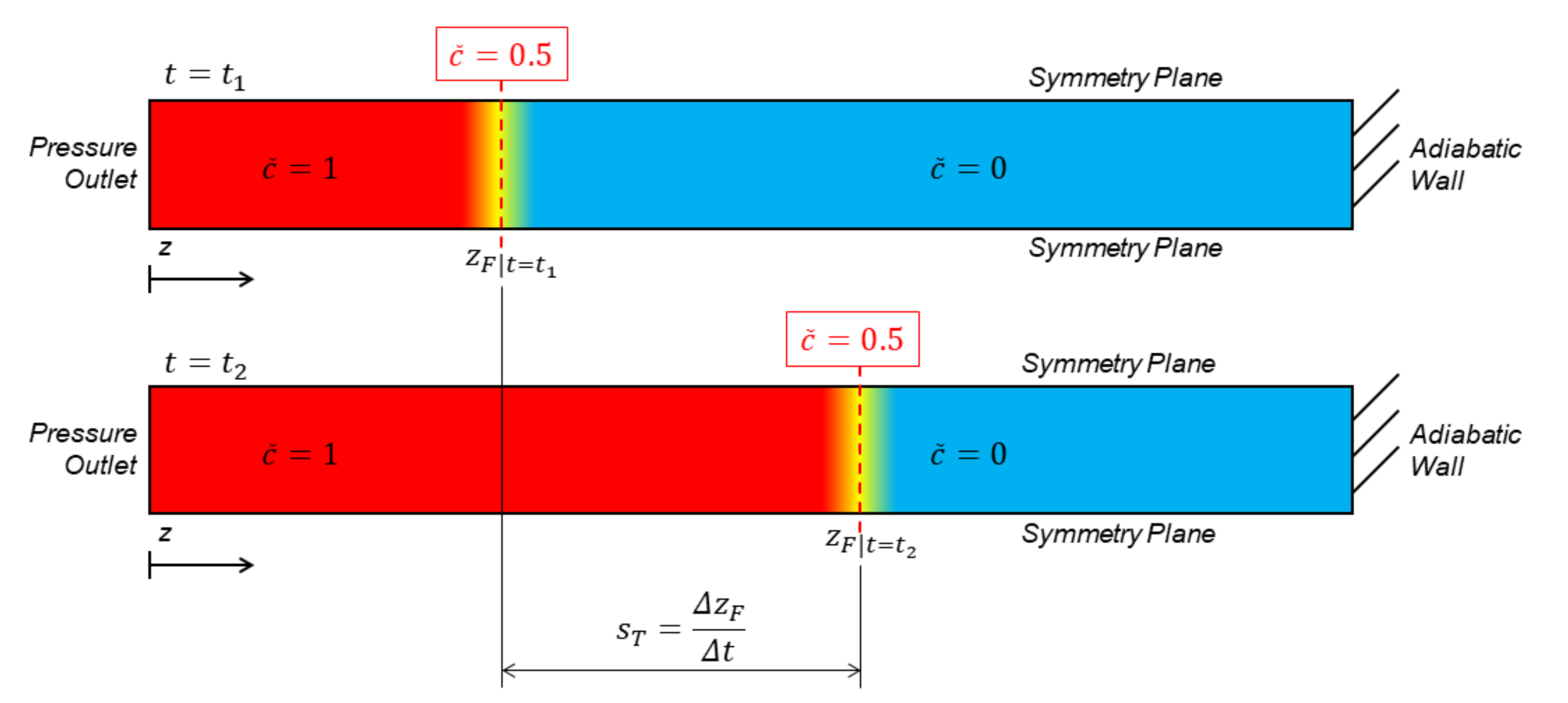
- The flame z-position for each iteration is elaborated for each simulation, and from Equation (1) is now .
- A region for the initial kernel growth (50 mm) is excluded from measurement: this is motivated by the need to consider only the steady-state portion of flame development, discarding the ignition treatment. Therefore, flame position and velocity data are only extracted for m.
- The simulation duration is 16 × 10−3 s, i.e., a sufficient physical time for steady-state turbulent flame development for all the investigated cases. This is chosen to be longer than engine time-scales for combustion completion.
- Turbulent flame speed is calculated as Combustion is initiated by a spark-ignition triggered at the first iteration from an ignition point on the domain z-axis at a 2 mm distance from the pressure outlet, and a spherical-type flame kernel is let to develop into a planar-like reaction front for measurement.
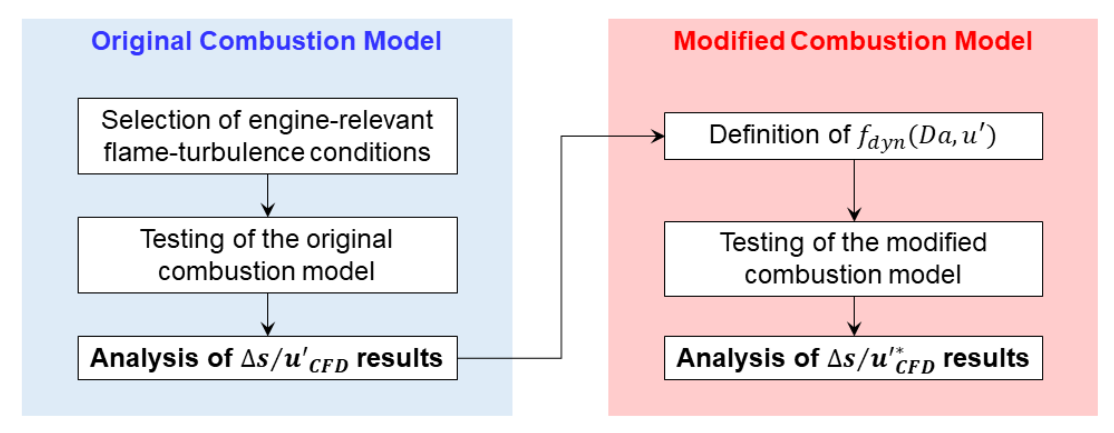
4. Methodology
- The non-dimensional group from the simulation results of the original combustion model (hereafter named ) is analytically reproduced by a function, obtained through a data-based analysis procedure.
- A reference function is identified from the literature (hereafter called . This serves as a physical basis for comparison with simulations. In this study, Equation (2) is considered as , although other correlations could be adopted.
- For each analysed combustion model, scaling on both and is compared to , and areas for model improvements are identified. An original dynamic function is defined, i.e., a new function in the space obtained from the data results to improve the turbulent burn rate of the combustion model. Based on this, a modified turbulent flame speed is obtained.
- All the simulations are repeated using and the results compared against literature data.
5. Results
6. Conclusions
Author Contributions
Funding
Conflicts of Interest
Nomenclature
| Combustion progress variable [-] | |
| CFR | Cooperative fuel research |
| CFL | Courant–Friedrichs–Lewy number |
| Normalized flame speed = [-] | |
| Normalized flame speed from simulations results (original model) [-] | |
| Normalized flame speed from simulations results (dynamic model) [-] | |
| Normalized flame speed from literature (reference) [-] | |
| Damköhler number [-] | |
| Mean Damköhler number [-] | |
| Laminar flame thickness [m] | |
| Energy dissipation rate [m2/s3] | |
| ECFM-3Z | Extended coherent flamelet model-3 zones |
| Turbulent kinetic energy [m2/s2] | |
| Karlovitz number [-] | |
| KPP | Kolmogorov–Petrovski–Piskunov |
| ICE | Internal combustion engines |
| Integral length scale [m] | |
| Turbulent viscosity [Pa s] | |
| Turbulent Reynolds number [-] | |
| SI | Spark ignition |
| Laminar flame speed [m/s] | |
| Turbulent flame speed [m/s] | |
| Target/modified turbulent flame speed from the literature (reference) [m/s] | |
| Ratio of turbulent to laminar flame speed [-] | |
| Ratio of turbulent/laminar flame speed from simulation results (original model) [-] | |
| Target ratio of turbulent/laminar flame speed from simulation results (modified dynamic model) [-] | |
| Target ratio of turbulent to laminar from the literature (reference) [-] | |
| Volumetric source term for momentum (vectorial) and temperature (scalar) transport equation | |
| Turbulence intensity [m/s] | |
| Position on the z-axis of the iso-surface [m] |
Appendix A

Appendix B

| 0.2940 | |
| 0.2332 | |
| 0.0909 | |
| 0.7009 | |
| −0.0580 | |
| 0.4668 | |
| 0.2987 | |
| 0.0476 | |
| −0.1488 | |
| 0.8517 | |
| 0.2824 |
References
- Peters, N. Turbulent Combustion; Cambridge University Press: Cambridge, UK, 2000. [Google Scholar]
- Peters, N. Laminar Flamelet Concepts in Turbulent Combustion; Fwenty-First Symposium (International) on Combustion/The Combustion Institute: Pittsburgh, PA, USA, 1986; pp. 1231–1250. [Google Scholar]
- Peters, N. The turbulent burning velocity for large-scale and small-scale turbulence. J. Fluid Mech. 1999, 384, 107–132. [Google Scholar] [CrossRef]
- Williams, F.A. A Review of Some Theoretical Considerations of Turbulent Flame Structure. AGARD Conf. Proc. 1975, 164, III-1–III-25. [Google Scholar]
- Colin, O.; Benkenida, A. The 3-Zone Extended Coherent Flame Model (ECFM3Z) for computing pre-mixed/diffusion combustion. Oil Gas Sci. Technol. Rev. IFP 2004, 59, 593–609. [Google Scholar] [CrossRef]
- Ewald, J.; Peters, N. On unsteady premixed turbulent burning velocity prediction in internal combustion engines. Proc. Combust. Inst. 2007, 31, 3051–3058. [Google Scholar] [CrossRef]
- Damköhler, G. The effect of turbulence on the flame velocities in gas mixtures. Z. Elektrochem. Angew. Phys. Chem. 1940, 46, 601–626. [Google Scholar]
- Damköhler, G. Der einfluß der turbulenz auf die flammengeschwindigkeit in gasgemischen. Z. Elektrochem. Angew. Phys. Chem. 1940, 46, 601–626. [Google Scholar]
- Abdel-Gayed, R.G.; Bradley, D.; Lawes, M. Turbulent burning velocities: A general correlation in terms of straining rates. Proc. R. Soc. Lond. Ser. A Math. Phys. Sci. 1987, 414, 389–413. [Google Scholar] [CrossRef]
- Bradley, D.; Lau, A.K.C.; Lawes, M.; Smith, F.T. Flame stretch rate as a determinant of turbulent burning velocity. Philos. Trans. R. Soc. A Math. Phys. Eng. Sci. 1992, 338, 359–387. [Google Scholar] [CrossRef]
- Bradley, D. How Fast Can We Burn? Twenty-Fourth Symposium (International) on Combustion/The Combustion Institute: Pittsburgh, PA, USA, 1992; pp. 247–262. [Google Scholar]
- Gülder, Ö.L. Turbulent Premised Combustion Modelling Using Fractal Geometry; Twenty-Third Symposium (International) on Combustion/The Combustion Institute: Pittsburgh, PA, USA, 1990; pp. 835–842. [Google Scholar]
- Gulder, O. Turbulent premixed flame propagation models for different combustion regimes. Symp. Combust. 1991, 23, 743–750. [Google Scholar] [CrossRef]
- Muppala, S.P.R.; Aluri, N.K.; Dinkelacker, F.; Leipertz, A. Development of an algebraic reaction rate closure for the numerical calculation of turbulent premixed methane, ethylene, and propane/air flames for pressures up to 1.0 Mpa. Combust. Flame 2005, 140, 257–266. [Google Scholar] [CrossRef]
- Burke, E.M.; Güthe, F.; Monaghan, R. A Comparison of Turbulent Flame Speed Correlations for Hydrocarbon Fuels at Elevated Pressures. In Turbo Expo: Power for Land, Sea, and Air; American Society of Mechanical Engineers: New York, NY, USA, 2016. [Google Scholar]
- Liu, C.-C.; Shy, S.S.; Peng, M.-W.; Chiu, C.-W.; Dong, Y.-C. High-pressure burning velocities measurements for centrally-ignited premixed methane/air flames interacting with intense near-isotropic turbulence at constant Reynolds numbers. Combust. Flame 2012, 159, 2608–2619. [Google Scholar] [CrossRef]
- Zimont, V.L. Gas premixed combustion at high turbulence. Turbulent flame closure combustion model. Exp. Therm. Fluid Sci. 2000, 21, 179–186. [Google Scholar] [CrossRef] [Green Version]
- Kobayashi, H. Experimental study of high-pressure turbulent premixed flames. Exp. Therm. Fluid Sci. 2002, 26, 375–387. [Google Scholar] [CrossRef]
- Ronney, P. Some open issues in premixed turbulent combustion. In Modeling in Combustion Science; Springer: Berlin/Heidelberg, Germany, 1955; pp. 1–22. [Google Scholar]
- Gülder, L. Contribution of small scale turbulence to burning velocity of flamelets in the thin reaction zone regime. Proc. Combust. Inst. 2007, 31, 1369–1375. [Google Scholar] [CrossRef]
- Wabel, T.M.; Skiba, A.W.; Driscoll, J.F. Turbulent burning velocity measurements: Extended to extreme levels of turbulence. Proc. Combust. Inst. 2017, 36, 1801–1808. [Google Scholar] [CrossRef] [Green Version]
- Wabel, T.M.; Skiba, A.W.; Temme, J.E.; Driscoll, J.F. Measurements to determine the regimes of premixed flames in extreme turbulence. Proc. Combust. Inst. 2017, 36, 1809–1816. [Google Scholar] [CrossRef] [Green Version]
- Hakberg, B.; Gosman, A. Analytical determination of turbulent flame speed from combustion models. Symp. Combust. 1985, 20, 225–232. [Google Scholar] [CrossRef]
- Fichot, F.; Lacas, F.; Veynante, D.; Candel, S. One-dimensional propagation of a premixed turbulent flame with the coherent flame model. Combust. Sci. Tech. 1993, 89, 1–26. [Google Scholar]
- Duclos, J.; Veynante, D.; Poinsot, T. A comparison of flamelet models for premixed turbulent combustion. Combust. Flame 1993, 95, 101–117. [Google Scholar] [CrossRef]
- Poinsot, T.; Veynante, D. Theoretical and Numerical Combustion, 2nd ed.; R.T. Edwards, Inc.: Morningside, QLD, Australia, 2005. [Google Scholar]
- Poludnenko, A.; Oran, E. The interaction of high-speed turbulence with flames: Global properties and internal flame structure. Combust. Flame 2010, 157, 995–1011. [Google Scholar] [CrossRef] [Green Version]
- Poludnenko, A.; Oran, E. The interaction of high-speed turbulence with flames: Turbulent flame speed. Combust. Flame 2011, 158, 301–326. [Google Scholar] [CrossRef] [Green Version]
- Wang, Z.; Magi, V.; Abraham, J. Turbulent Flame Speed Dependencies in Lean Methane-Air Mixtures under Engine Relevant Conditions. Combust. Flame 2017, 180, 53–62. [Google Scholar] [CrossRef]
- Iacovano, C.; D’Adamo, A.; Cantore, G. Analysis and Simulation of Non-Flamelet Turbulent Combustion in a Research Optical Engine. Energy Procedia 2018, 148, 463–470. [Google Scholar] [CrossRef]
- Bradley, D.; Lawes, M.; Mansour, M.S. Correlation of turbulent burning velocities of ethanol–air, measured in a fan-stirred bomb up to 1.2 Mpa. Combust. Flame 2011, 158, 123–138. [Google Scholar] [CrossRef]
- Bradley, D.; Lawes, M.; Mansour, M.S. The Problems of the Turbulent Burning Velocity. Flow Turbul. Combust. 2011, 87, 191–204. [Google Scholar] [CrossRef]
- Gillespie, L.; Lawes, M.; Sheppard, C.G.W.; Woolley, R. Aspects of Laminar and Turbulent Burning Velocity Relevant to SI Engines. SAE Trans. 2000, 109, 13–33. [Google Scholar]
- D’Adamo, A.; Del Pecchia, M.; Breda, S.; Berni, F.; Fontanesi, S.; Prager, J. Chemistry-Based Laminar Flame Speed Correlations for a Wide Range of Engine Conditions for Iso-Octane, n-Heptane, Toluene and Gasoline Surrogate Fuels. In Proceedings of the SAE 2017 International Powertrains, Fuels and Lubricants Meeting, Beijing, China, 16–19 October 2017. [Google Scholar]
- Colin, O.; Chevillard, S.; Bohbot, J.; Senecal, P.K.; Pomraning, E.; Wang, M. Development of a Species-Based Extended Coherent Flamelet Model (SB-ECFM) for Gasoline Direct Injection Engine (GDI) Simulations. In Proceedings of the Internal Combustion Engine Division Fall Technical Conference, San Diego, CA, USA, 4–7 November 2018; Volume 2. [Google Scholar] [CrossRef]
- Lucchini, T.; Cornolti, L.; Montenegro, G.; D’Errico, G.; Fiocco, M.; Teraji, A.; Shiraishi, T. A Comprehensive Model to Predict the Initial Stage of Combustion in SI Engines. SAE Tech. Pap. 2013. [Google Scholar] [CrossRef]
- Zhu, X.; Sforza, L.; Ranadive, T.; Zhang, A.; Lee, S.-Y.; Naber, J.; Lucchini, T.; Onorati, A.; Anbarasu, M.; Zeng, Y. Experimental and Numerical Study of Flame Kernel Formation Processes of Propane-Air Mixture in a Pressurized Combustion Vessel. SAE Int. J. Engines 2016, 9, 1494–1511. [Google Scholar] [CrossRef]
- Falfari, S.; Bianchi, G.M. Development of an Ignition Model for S.I. Engines Simulation. SAE Tech. Pap. 2007. [Google Scholar] [CrossRef]
- D’Adamo, A.; Breda, S.; Fontanesi, S.; Cantore, G. A RANS-Based CFD Model to Predict the Statistical Occurrence of Knock in Spark-Ignition Engines. SAE Int. J. Engines 2016, 9, 618–630. [Google Scholar] [CrossRef]
- D’Adamo, A.; Breda, S.; Fontanesi, S.; Irimescu, A.; Merola, S.S.; Tornatore, C. A RANS knock model to predict the statistical occurrence of engine knock. Appl. Energy 2017, 191, 251–263. [Google Scholar] [CrossRef]
- D’Adamo, A.; Breda, S.; Iaccarino, S.; Berni, F.; Fontanesi, S.; Zardin, B.; Borghi, M.; Irimescu, A.; Merola, S.S. Development of a RANS-Based Knock Model to Infer the Knock Probability in a Research Spark-Ignition Engine. SAE Int. J. Engines 2017, 10, 722–739. [Google Scholar] [CrossRef]
- Forte, C.; Bianchi, G.M.; Corti, E.; Fantoni, S.; Costa, M. CFD Methodology for the Evaluation of Knock of a PFI Twin Spark Engine. Energy Procedia 2014, 45, 859–868. [Google Scholar] [CrossRef] [Green Version]
- Breda, S.; D’Orrico, F.; Berni, F.; D’Adamo, A.; Fontanesi, S.; Irimescu, A.; Merola, S.S. Experimental and numerical study on the adoption of split injection strategies to improve air-butanol mixture formation in a DISI optical engine. Fuel 2019, 243, 104–124. [Google Scholar] [CrossRef]
- Breda, S.; D’Adamo, A.; Fontanesi, S.; D’Orrico, F.; Irimescu, A.; Merola, S.S.; Giovannoni, N. Numerical Simulation of Gasoline and n-Butanol Combustion in an Optically Accessible Research Engine. SAE Int. J. Fuels Lubr. 2017, 10, 32–55. [Google Scholar] [CrossRef]
- Breda, S.; Berni, F.; D’Adamo, A.; Testa, F.; Severi, E.; Cantore, G. Effects on Knock Intensity and Specific Fuel Consumption of Port Water/Methanol Injection in a Turbocharged GDI Engine: Comparative Analysis. Energy Procedia 2015, 82, 96–102. [Google Scholar] [CrossRef] [Green Version]
- Del Pecchia, M.; Pessina, V.; Berni, F.; D’Adamo, A.; Fontanesi, S. Gasoline-ethanol blend formulation to mimic laminar flame speed and auto-ignition quality in automotive engines. Fuel 2020, 264, 116741. [Google Scholar] [CrossRef]
- Fontanesi, S.; Cicalese, G.; D’Adamo, A.; Pivetti, G. Validation of a CFD Methodology for the Analysis of Conjugate Heat Transfer in a High Performance SI Engine. SAE Tech. Pap. 2011. [Google Scholar] [CrossRef]
- Berni, F.; Fontanesi, S.; Cicalese, G.; D’Adamo, A. Critical Aspects on the Use of Thermal Wall Functions in CFD In-Cylinder Simulations of Spark-Ignition Engines. SAE Int. J. Commer. Veh. 2017, 10, 547–561. [Google Scholar] [CrossRef]
- Berni, F.; Cicalese, G.; Fontanesi, S. A modified thermal wall function for the estimation of gas-to-wall heat fluxes in CFD in-cylinder simulations of high performance spark-ignition engines. Appl. Therm. Eng. 2017, 115, 1045–1062. [Google Scholar] [CrossRef]
- Koch, J.; Xu, G.; Wright, Y.M.; Boulouchos, K.; Schiliro, M. Comparison and Sensitivity Analysis of Turbulent Flame Speed Closures in the RANS G-Equation Context for Two Distinct Engines. SAE Int. J. Engines 2016, 9, 2091–2106. [Google Scholar] [CrossRef]
- Pal, P.; Kolodziej, C.; Choi, S.; Som, S.; Broatch, A.; Gomez-Soriano, J.; Wu, Y.; Lu, T.; See, Y.C. Development of a Virtual CFR Engine Model for Knocking Combustion Analysis. SAE Int. J. Engines 2018, 11, 1069–1082. [Google Scholar] [CrossRef]
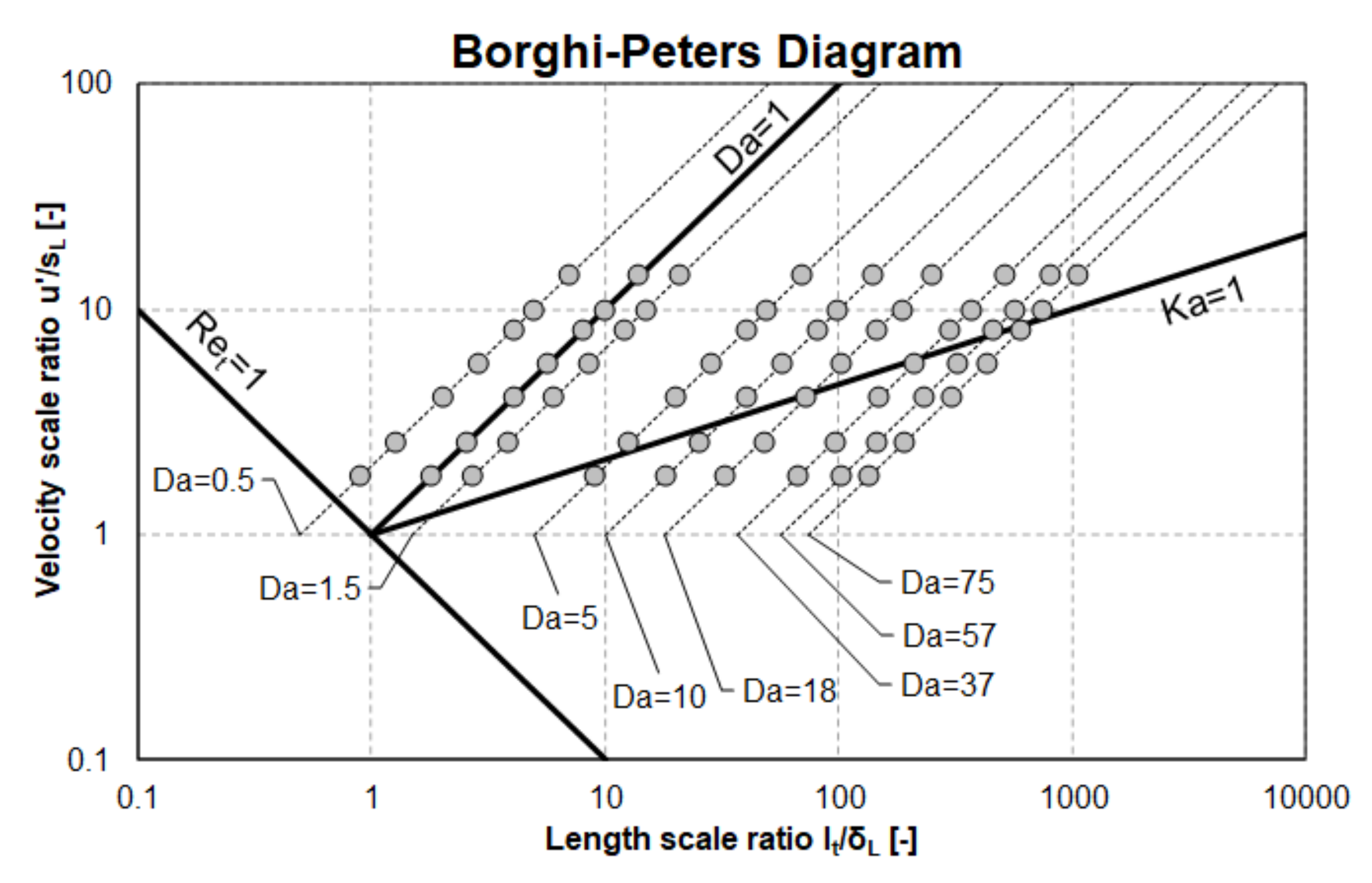

| Da | u′/sL = 1.83 | u′/sL = 2.58 | u′/sL = 4.08 | u′/sL = 5.77 | u′/sL = 8.16 | u′/sL = 10 | u′/sL = 14.14 |
|---|---|---|---|---|---|---|---|
| 0.5 | ε = 2.24 × 10⁵ | ε = 4.47 × 10⁵ | ε = 1.12 × 10⁶ | ε = 2.24 × 10⁶ | ε = 4.47 × 10⁶ | ε = 6.71 × 10⁶ | ε = 1.342 × 10⁷ |
| 1 | ε = 1.12 × 10⁵ | ε = 2.24 × 10⁵ | ε = 5.59 × 10⁵ | ε = 1.12 × 10⁶ | ε = 2.24 × 10⁶ | ε = 3.35 × 10⁶ | ε = 6.708 × 10⁶ |
| 1.5 | ε = 7.45 × 10⁴ | ε = 1.49 × 10⁵ | ε = 3.73 × 10⁵ | ε = 7.45 × 10⁵ | ε = 1.49 × 10⁶ | ε = 2.24 × 10⁶ | ε = 4.472 × 10⁶ |
| 5 | ε = 2.24 × 10⁴ | ε = 4.47 × 10⁴ | ε = 1.12 × 10⁵ | ε = 2.24 × 10⁵ | ε = 4.47 × 10⁵ | ε = 6.71 × 10⁵ | ε = 1.342 × 10⁶ |
| 10 | ε = 1.12 × 10⁴ | ε = 2.24 × 10⁴ | ε = 5.59 × 10⁴ | ε = 1.12 × 10⁵ | ε = 2.24 × 10⁵ | ε = 3.35 × 10⁵ | ε = 6.708 × 10⁵ |
| 18 | ε = 6.21 × 10³ | ε = 1.24 × 10⁴ | ε = 3.11 × 10⁴ | ε = 6.21 × 10⁴ | ε = 1.24 × 10⁵ | ε = 1.86 × 10⁵ | ε = 3.727 × 10⁵ |
| 37 | ε = 3.02 × 10³ | ε = 6.04 × 10³ | ε = 1.51 × 10⁴ | ε = 3.02 × 10⁴ | ε = 6.04 × 10⁴ | ε = 9.07 × 10⁴ | ε = 1.813 × 10⁵ |
| 57 | ε = 1.96 × 10³ | ε = 3.92 × 10³ | ε = 9.81 × 10³ | ε = 1.96 × 10⁴ | ε = 3.92 × 10⁴ | ε = 5.88 × 10⁴ | ε = 1.177 × 10⁵ |
| 75 | ε = 1.49 × 10³ | ε = 2.98 × 10³ | ε = 7.45 × 10³ | ε = 1.49 × 10⁴ | ε = 2.98 × 10⁴ | ε = 4.47 × 10⁴ | ε = 8.944 × 10⁴ |
Publisher’s Note: MDPI stays neutral with regard to jurisdictional claims in published maps and institutional affiliations. |
© 2021 by the authors. Licensee MDPI, Basel, Switzerland. This article is an open access article distributed under the terms and conditions of the Creative Commons Attribution (CC BY) license (https://creativecommons.org/licenses/by/4.0/).
Share and Cite
d’Adamo, A.; Iacovano, C.; Fontanesi, S. A Data-Driven Methodology for the Simulation of Turbulent Flame Speed across Engine-Relevant Combustion Regimes. Energies 2021, 14, 4210. https://doi.org/10.3390/en14144210
d’Adamo A, Iacovano C, Fontanesi S. A Data-Driven Methodology for the Simulation of Turbulent Flame Speed across Engine-Relevant Combustion Regimes. Energies. 2021; 14(14):4210. https://doi.org/10.3390/en14144210
Chicago/Turabian Styled’Adamo, Alessandro, Clara Iacovano, and Stefano Fontanesi. 2021. "A Data-Driven Methodology for the Simulation of Turbulent Flame Speed across Engine-Relevant Combustion Regimes" Energies 14, no. 14: 4210. https://doi.org/10.3390/en14144210