Distributed Nonlinear AIMD Algorithms for Electric Bus Charging Plants

Abstract

Recently, the introduction of electric vehicles has given rise to a new paradigm in the transportation field, spurring the public transport service in the direction of using completely electric bus fleets. In this context, one of the main challenges is that of guaranteeing an optimal scheduling of the charging process, while reducing the power supply requested from the main grid, and improving the efficiency of the resource allocation. Therefore, in this paper, a power allocation strategy is proposed in order to optimize the charging of electric bus fleets, while fulfilling the limitation imposed on the maximum available power, as well as ensuring limited charging times. Specifically, relying on real bus charging scenarios, a charging optimization algorithm based on a Nonlinear Additive Increase Multiplicative Decrease (NAIMD) strategy is proposed and discussed. This approach is designed on the basis of real charging power curves related to the batteries of the considered vehicles. Moreover, the adopted NAIMD algorithm allows us to minimize the sum of charging times in the presence of saturation constraints in a distributed way and with a small amount of aggregated data sent over the communication network. Finally, an extensive simulation campaign is illustrated, showing the effectiveness of the proposed approach both in allocating the power resources and in sizing the maximum power capacity of charging plants in progress.

1. Introduction

In recent years, the development of new means of transportation based on a more sustainable source of energy rather than fossil fuel has given rise to a new paradigm in mobility [1]. There is indeed a clear trend towards the realization of electric vehicles (EVs), which allow us to achieve economical and environmental benefits, in terms of both energy efficiency and the reduction of carbon emissions.

1.1. Motivation and Objective

Because of the intermittence of the charging process and the need of new architectures for the power supply, optimal resource allocation strategies are required to address issues such as power control and loss minimization [2]. Furthermore, the spread of EVs in the coming years will give rise to a gradual replacement of fuel pumps with electric charging stations. Hence, the study of new charging infrastructures and technologies capable of making the charging process faster, while preserving the life of the batteries, is nowadays a key challenge. Additionally, an optimal coordination between the charging processes needs to be guaranteed in order to significantly reduce possible negative effects on the main power grid, while improving the power supply reliability and the resource allocation efficiency (see, for instance, Ref. [3] for a recent review on the topic). All these aspects therefore motivate the present work, so that the main objective is the design of an efficient and flexible power allocation strategy able to take into account not only the battery dynamics to improve the charging process but also charging time limits to allow electric bus fleets to perform their daily service without interruptions.

1.2. Literature Overview

The optimal management of EV charging has been widely investigated in the literature, where centralized, decentralized or distributed control approaches have been proposed (see, e.g., [4,5,6,7,8,9,10,11,12,13,14], among many others).

In the centralized schemes, the charging stations collect information about the state of all the vehicles (e.g., state of charge, arrival time or saturation power of the batteries), and then transmit them to a central control unit, which provides a suitable scheduling of the charging process in order to satisfy specific objectives and constraints. In [4], for instance, an optimization problem is solved to coordinate the choice of EV charging station in the case of long-distance trips, while reducing the waiting time for charging. In [5], instead, electric bus fast-charging stations with a stationary energy storage system are considered, and an optimization problem is solved to achieve the optimal sizes of the energy buffer to cope with uncertainties on arrival time and state of charge due to different factors such as actual traffic conditions. In [6], a method to coordinate the charging of EVs and shift the load demand from the peak period to the valley period is introduced, taking also into account indicators on different charging demand urgency for ensuring some charging priority among vehicles. The minimization of the power losses, the mitigation of the risk associated with the energy trading and the maximization of the operation profits during the charging process are also investigated, for instance, in [7,8].

As for the decentralized and distributed approaches, the central control system broadcasts common power references to all radial subsystems, where a suitable charging power is locally provided to the connected EVs, based on their own internal parameters and optimization criteria. Among the decentralized control architectures in the literature, in [9], a strategy to coordinate the EV charging by exploiting the concepts of non-cooperative and multi evolutionary games is discussed, and a price-based strategy is designed. A decentralized EV charging control, based on the augmented Lagrangian method, is instead proposed in [10] in order to achieve the maximum revenue, while taking into account the distribution network constraints. Since the uncoordinated charging of large-scale EVs may cause high load peak of power at rush hours, thus implying a growth in the cost of electricity, a possible solution, while keeping the same charging infrastructure, is to shift the peak power demands to off-peak hours, as in [11]. A method based on the use of a probabilistic transition matrix to update the charging process is adopted in [12]. In [13], a communication-free droop control approach, which relies on the local measurements of voltage at the point of connection, is adopted to determine the charging power for the EVs. In [14], a deep reinforcement learning-based method for the minimization of individual EV charging costs is proposed.

A recent decentralized solution which does not require any communication or needs only a small amount of information about the agents is represented by the so-called Additive Increase Multiplicative Decrease (AIMD) algorithms [15,16]. These are indeed capable of providing an optimal resource allocation strategy in the presence of saturation constraints for each user connected to the same infrastructure. AIMD approaches for EV charging have been proposed in the literature, as in [17,18,19,20,21], among others. For instance, in [20], a mixed distributed power allocation solution is provided so as to capture the main advantages of optimal algorithms which minimize either the sum of charging times or the recharging time for each vehicle. Meanwhile, in [17], a fixed number of vehicles connected to the network is considered, and in [20], the AIMD algorithm is applied to a coordinate charging process in a scenario characterized by random energy requirements and a random number of connecting vehicles. In all these works, the evolution of the charging rate is assumed to be linear, but in practice, a non-linear charging curve should be considered to take into account the real physical behaviour of the system. This also motivates the present work, where a nonlinear model of the charging process is considered, and an NAIMD approach is adopted to ensure optimal resource allocation for electric bus charging plants.

1.3. Contributions

This paper proposes an optimal power allocation strategy capable of coordinating the charging process of an electric bus fleet in a scenario in which the available power provided by the electric grid is limited. Since increasing the size of the electrical plant to which the charging spots are connected can be significantly expensive, the management of the power distribution among the electric vehicles is in fact mandatory. Therefore, the AIMD algorithm is ideal to solve this problem, also being able to satisfy predefined constraints on the charging times. Differently from previous works as in [20,21], the proposed algorithm is designed to reproduce the characteristic power curves of the bus batteries and their saturation (further details can be found in [22]). The proposal is theoretically discussed relying on the NAIMD theory in [15] (Chapter 11), and its properties are verified on a charging scenario based on real data from an existing bus charging plant in Milan, Italy. Moreover, the effectiveness of the proposal is also exploited to size the maximum power of a new charging plant in Alessandria, Italy. Specifically, a reverse engineering problem is solved to find the most suitable minimum grid capacity so as to satisfy predefined requirements on the charging times of a bus fleet.

1.4. Outline of the Paper

The paper is organized as follows. In Section 2, some preliminaries on classical AIMD and the adopted NAIMD algorithms are recalled. The description of the charging process and of the considered vehicles is reported in Section 3. In Section 4, the proposed NAIMD strategy is introduced and analyzed, while in Section 5, different simulations, carried out on two different case studies of Italian cities, are illustrated and commented on to assess the proposal. Some conclusions are finally gathered in Section 6.

2. Methodology and Preliminaries

In this section, some preliminaries on the AIMD algorithm and its nonlinear extension, i.e., the NAIMD approach, are recalled.

The AIMD algorithm is in fact an efficient distributed approach capable of allocating the shares of a limited constrained resource among many agents by exploiting the limited communication among them. While AIDM algorithms were originally applied for congestion avoidance in computer networks [23], by virtue of their scalability and flexibility, they have been applied even in different contexts, such as that of battery recharging and power grids, where many users (e.g., EVs as in this paper or distributed generation units) connected to the same infrastructure have to share a resource (e.g., power). The only information given to the users is the notification that the available resource has reached its capacity limit. As a consequence, each agent, locally and independently, can recompute its power share to fulfil the whole limit.

This conceptual framework is hereafter mathematically formalized, for the readers’ convenience. Specifically, consider a multi-agent system where $N\in {\mathbb{N}}^{+}$ users are connected to the same architecture and share a resource at time $t\in {\mathbb{R}}_0^{+}$. Let $p_i\left(t\right)$ be the share of the ith user at time t, and $\overline{P}$ be the maximum available demand of resource such that

$$\sum _{i=1}^N{p}_i\left(t\right)=P\le \overline{P},\forall t\ge t_0.$$

(1)

According to the AIMD working principle introduced in [15], if at the time instant $t=t_k$, $k\in {\mathbb{N}}_0^{+}$, it holds that

$$P=\overline{P},$$

(2)

therefore, a capacity event (CE) occurs, and a share allocation is required.

2.1. AIMD Algorithm

Relying on the theory introduced in [15] (Chapter 1), the classical AIMD strategy allows such allocation in a completely decentralized way, without requiring any information about the state of the agents, but only the knowledge of the triggering event provided by an event detector. More precisely, the classical synchronized AIMD approach consists of two phases, called Additive Increase (AI) and Multiplicative Decrease (MD), respectively.

Let ${\alpha }_i\in {\mathbb{R}}^{+}$, and ${\beta }_i\in (0,1]$, with $i=1,\dots ,N$, be the so-called growth factors and multiplicative factors, respectively. Then, during the AI phase, the AIMD evolution is captured by the following linear model, i.e.,

$$p_i\left(t\right)={\beta }_i{p}_i\left(t_k\right)+{\alpha }_i(t-t_k),\forall i=1,\dots ,N,$$

(3)

with $t_k\le t<t_{k+1}$. Whenever a CE (2) occurs, instead, the MD phase is activated and all the users instantaneously decrease their resource share by the factor ${\beta }_i$, so that

$$p_i\left(t_k^{+}\right)={\beta }_i{p}_i\left(t_k^{-}\right),$$

(4)

with $p_i\left(t_k^{+}\right)$ and $p_i\left(t_k^{-}\right)$ being the right and left limit of $p_i\left(t\right)$ in $t_k$. As a consequence, the dynamics between two CEs is given by

$$p_i\left(t_{k+1}\right)={\beta }_i{p}_i\left({\tau }_k\right)+{\alpha }_i{T}_k,$$

(5)

where $T_k=t_{k+1}-t_k$ is the so-called inter-capacity time, and

$$T_k=\frac{1}{{\sum }_{j=1}^N{\alpha }_j}\sum _{j=1}^N(1-{\beta }_j)p_j\left({\tau }_k\right).$$

(6)

Hence, substituting (6) into (5), it is possible to write the corresponding discrete time linear system defined at the CEs and captured by

$$p\left(t_{k+1}\right)=Ap\left(t_k\right),$$

(7)

where $p={[p_1,\dots ,p_N]}^{\top }\in {\mathbb{R}}^N$ such that ${\sum }_{i=1}^N{p}_i=\overline{P}$, while the matrix A is given by

$$A=\mathrm{diag}\left(\beta \right)+{\left({\mathrm{𝟙}}^{\top }\alpha \right)}^{-1}\alpha {(\mathrm{𝟙}-\beta )}^{\top },$$

(8)

with $\mathrm{𝟙}$ being the vector of all ones, $\alpha =[{\alpha }_1,\dots ,{\alpha }_N]\in {\mathbb{R}}^N$ and $\beta =[{\beta }_1,\dots ,{\beta }_N]\in {\mathbb{R}}^N$.

2.2. NAIMD Algorithm

Intending to design an optimal allocation strategy for the battery charging of EVs, which is characterized by a nonlinear dynamics (see e.g., [24]), the so-called NAIMD algorithm naturally applies. Moreover, in order to take into account the physical limit of the considered batteries, constraints on the shared power by each user are hereafter considered.

Differently from the linear AIMD algorithm, in the case of the NAIMD version, the increase phase is captured by a nonlinear function, so that the time evolution between two CEs is given by

$$p_i\left(t\right)=f_i(p_i\left(t_k\right),t-t_k),\forall i=1,\dots ,N,$$

(9)

where $f_i(·,·)$ is a function of the share and of time, and $p\left(t\right)\in \mathcal{P}$ with

$$\mathcal{P}\triangleq \left\{p\in {\mathbb{R}}^N\mid {\underline{p}}_i\le p_i\le {\overline{p}}_i\right\},$$

(10)

and ${\underline{p}}_i$ and ${\overline{p}}_i$ being the lower and upper bounds, respectively. Let now G be any continuous and strictly increasing function defined in $\mathcal{P}$, called the capacity function. Analogously to the linear AIMD approach, each user increases its share until the total available capacity is achieved, i.e., a CE occurs at $t=t_k$, if

$$G(p_1\left(t_k\right),\dots ,p_N\left(t_k\right))=\overline{P}.$$

(11)

Therefore, the users are notified that the maximum capacity has been reached and they reduce the share according to (4). The corresponding dynamics at the CEs is instead given by

$$p_i\left(t_{k+1}\right)=f_i(p_i\left(t_k\right),T_k),\forall i=1,\dots ,N,$$

(12)

where $T_k$ is the kth inter-capacity time. Letting $F(p,t-t_k)={[f_1(p_1,t-t_k),\dots ,f_N(p_N,t-t_k)]}^{\top }$, the NAIMD discrete dynamics at the CEs is then modeled as

$$p\left(t_{k+1}\right)=F(p\left(t_k\right),T_k)$$

(13)

with $F(p,0)$ being the vector-valued function of the share at $t=t_k,\forall k\in {\mathbb{N}}_0^{+}$.

3. Charging Process and Bus Characteristics

In order to formulate the power allocation problem for charging electric bus fleets in a public scenario, it is instrumental to define the functional roles and characteristics of the power plant operator, which defines the appropriate charging strategies in advance. More specifically, in this section, the considered bus fleets and depot characteristics are described.

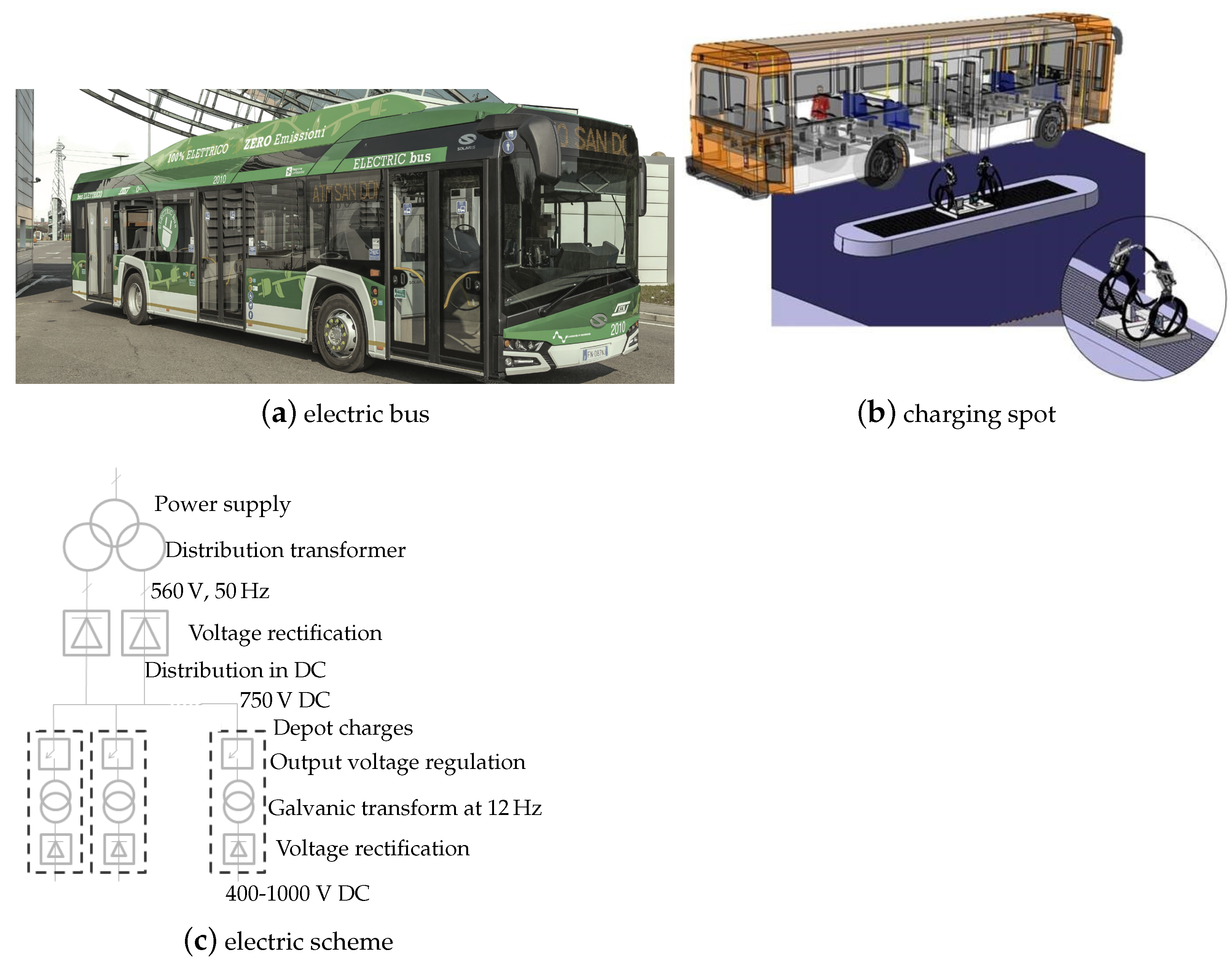
3.1. Power Plant and Depot Characteristics

The operational schedules of the charging process as well as the power plant features are hereafter discussed. Typically, two charging concepts can be considered (see, e.g., [25,26] for further details):

• charging is executed after the service time when the buses are parked on the shunting area inside the depot;
• charging is also possible during the service time, by means of fast-charging spots at terminal stations.

Specifically, in this work, the first operative mode is deeply analyzed. In fact, since the depot area realized for bus recharging is limited, it is essential to optimize the available spaces in order to install the charging spots, as those illustrated in Figure 1.

The amount of spots is in general greater than or equal to the number of the vehicles so that, when a bus arrives at the depot, it can be directly connected to the electric grid for recharging. Moreover, differently from charging during service, which is as fast as possible, the buses at the final depot can be kept contemporarily connected to their spots until their next daily service.

Therefore, it is crucial to provide the suitable power for the bus charging, while accounting for the power limit, the time constraints, the number of vehicles and their residual charge. This role is played by a dedicated supervisory control and data acquisition (SCADA) tool, which represents the so-called energy management system (EMS). On the basis of each type of battery fastened on the electric buses and their power characteristic curves, the EMS has to determine the optimal allocation and charging profile. In particular, the SCADA tool collects information about the battery state of charge (SOC), energy consumption during the charging process and the profile associated with the maximum charging power, and then it generates the correct values of current and voltage as set-points for the charging spots. Moreover, additional constraints can be imposed on the battery power in order to avoid phenomena such as overheating of electrical components.

As for the electric architecture of the charging station, a distribution transformer converts the high-voltage electricity from the main grid to a lower voltage level for household and commercial use. Then, the AC current is converted by a specific rectifier into a DC current. As illustrated in Figure 1c, the charging spots are characterized by a DC current with voltage equal to 750 V. Each depot charger is in turn composed of three elements: the output voltage regulator converts the DC current into an AC current; then, a galvanic insulation transformer with ratio 1:1 transfers the charging power to the bus, while isolating it from the power source; finally, the AC current is converted by a rectifier into a DC current and then it flows towards the recharge plug, where the bus is connected.

3.2. Bus Characteristics

In order to describe the characteristics of the batteries involved in the charging process, without loss of generality, consider the curves in Figure 2a,b, where ${\iota }_i$ is the input current, $p_i$ is the charging rate with respect to the input voltage $v_i$, and ${\overline{\iota }}_i$ and ${\overline{p}}_i$ are the corresponding maximum values. Therefore, the charging process is active until each battery reaches its maximum energy capacity, namely ${\overline{E}}_i$, so that the corresponding bus can be disconnected.

Each battery has a maximum capacity of 304 $\mathrm{k}$$\mathrm{W}$$\mathrm{h}$, and it is possible to observe that, during charging, the current is kept constant, while the charging power linearly increases with respect to the voltage up to the saturation value of 100 $\mathrm{k}$$\mathrm{W}$. Once the saturation value is reached, the current reduces in order to keep the absorbed power constant till the end of the charging process. Since the power plant is characterized by a maximum power capacity, namely $\overline{P}$, during this process, the charging rate cannot indefinitely increase, but specific constraints in terms of power and charging time have to be fulfilled so as to have the sum of charging rates equal to or smaller than $\overline{P}$.

3.3. The Charging Rate Allocation Problem

Consider now a bus depot with N buses connected to the charging spots, and assume, without loss of generality, that their batteries are identical. We are now in a position to formulate the charging rate allocation problem. Given the maximum power $\overline{P}$ of the charging plant, at each time step, it is required that (1) holds, while fulfilling the power constraint (10) defined for each vehicle. Moreover, having in mind a public transportation system, each electric bus has to be recharged only in a specific time interval, defined as ${\mathcal{T}}_{\mathrm{c}i}\triangleq [{\underline{t}}_i,{\overline{t}}_i]$, after the daily service.

4. The Adopted NAIMD Algorithm

In this paper, to solve the problem previously formulated, we propose an NAIMD algorithm of the type introduced in Section 2.2.

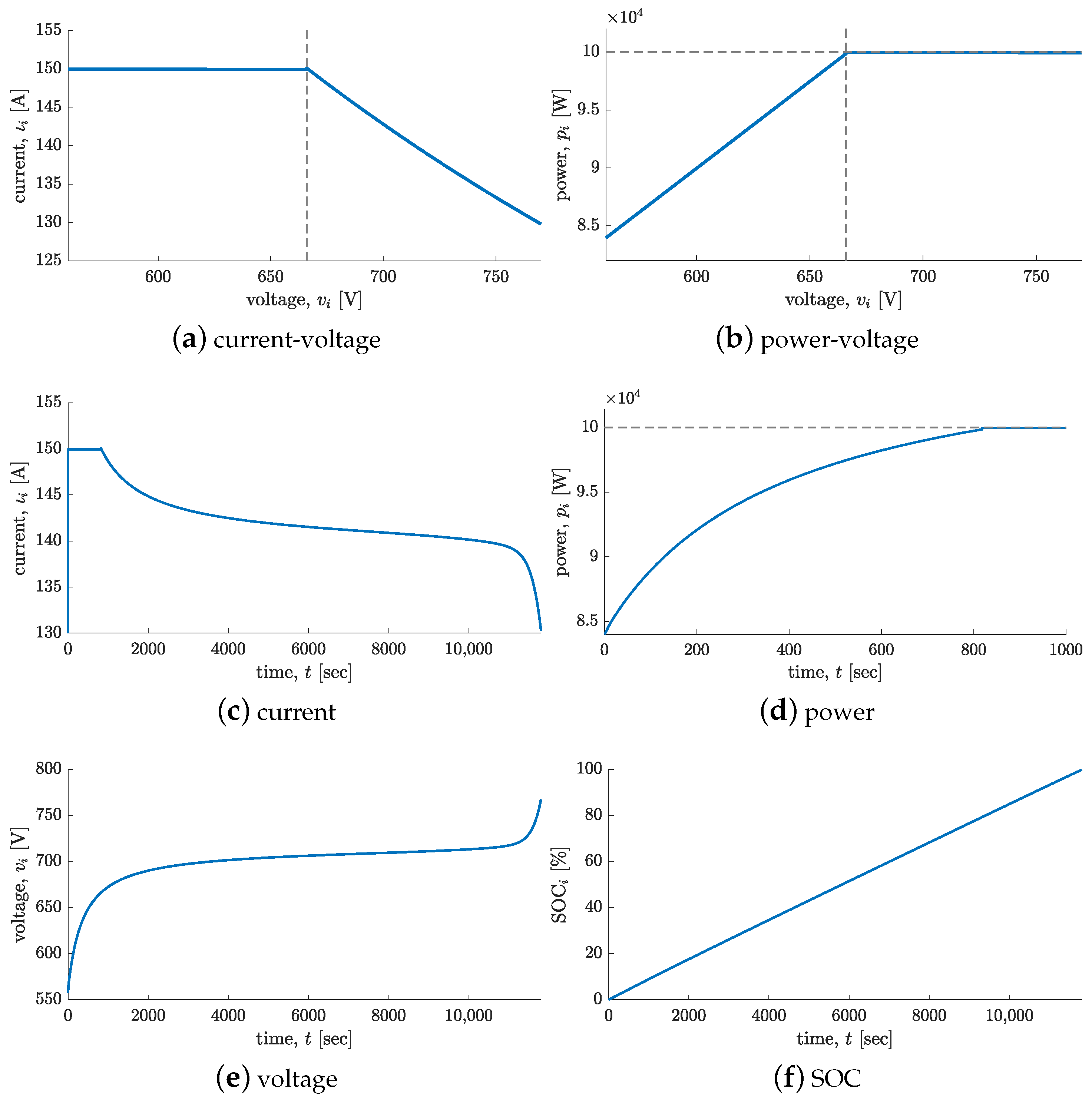
4.1. Recast of the Battery Model in the NAIMD Framework

In order to design the NAIMD algorithm, the model of the battery represented by the charging curve in Figure 2d needs to be suitably defined. As mentioned before, such a curve presents an exponential evolution until the saturation value, and then the power is kept constant up to the end of the charging process. Hence, to find a simple model of the charging rate, a polynomial regression is adopted as follows,

$$p_i\left(t\right)\approx \sum _{j=0}^n{c}_j{t}^j,\forall i=1,\dots ,N,$$

(14)

with $c_j\in \mathbb{R}$ being the parameters to determine, for instance, via the Least Square (LS) method, and n being the order of the selected polynomial.

Letting $n=3$ and considering the interval $[0,{\overline{t}}_{\mathrm{s}}]$, with ${\overline{t}}_{\mathrm{s}}$ being the time when the power saturates, the model of the charging power curve used in this work is captured by

$$p_i\left(t\right)\approx \left\{\begin{array}{cc}{c}_0+c_{1}t+c_2{t}^2+c_3{t}^3,\hfill & \forall t<{\overline{t}}_{\mathrm{s}}\hfill \\ {\overline{p}}_i,\hfill & \forall t>{\overline{t}}_{\mathrm{s}}\hfill \end{array}\right..$$

(15)

Given the battery model (15), the charging rate allocation problem formulated in Section 3.3 can be now recast into the NAIMD framework. Specifically, the continuous dynamics of the charging rate leads to the NAIMD model (9), with

$$f_i(p_i\left(t_k\right),t-t_k)=\left\{\begin{array}{cc}{\beta }_i{p}_i\left(t_k\right)+c_1(t-t_k)+c_2{(t-t_k)}^2+c_3{(t-t_k)}^3,\hfill & p_i\left(t\right)<{\overline{p}}_i\hfill \\ {\overline{p}}_i,\hfill & p_i\ge {\overline{p}}_i\hfill \end{array}\right.,$$

(16)

$\forall i=1,\dots ,N$, where the coefficients $c_1,c_2$ and $c_3$ can be found online by using the LS method at each CE, as previously mentioned. Specifically, the CE occurs whenever condition (11) holds, with function G defined as

$$G({\sigma }_1,\dots ,{\sigma }_N)\triangleq {\mathrm{𝟙}}^{\top }\sigma ,$$

(17)

with $\sigma \triangleq {[{\sigma }_1,\dots ,{\sigma }_N]}^{\top }\in {\mathbb{R}}^N$ a suitable positive vector.

Remark 1

(Implementation practices). Note that, although classical AIMD formulations are given in a continuous-time framework, a discretization is needed for practical implementation (see also [20]). Therefore, letting $h\in {\mathbb{N}}_{\ge 0}$ be the discrete time step, with T being the sampling time, one can write

$$p_i\left[h\right]=p_i\left(t\right),\forall t\in [hT,(h+1)T).$$

(18)

4.2. Minimization of the Sum of Charging Times

Consider that the N buses connected to the charging spots at the time instant h share the available constant power $\overline{P}$. Let $h_{\mathrm{c}i}$ be the time that the ith user takes to complete the charging, and let $E_i^{★}$ be the total amount of the desired energy to be supplied to user i. Hence, the minimization of the charging times is achieved by defining the cost function

$$J\left(N\right)=\sum _{i=1}^N{h}_{\mathrm{c}i},$$

(19)

and solving the following optimal control problem

$$\begin{array}{cc}\hfill & \underset{p_i\left[h\right]}{min}J\left(N\right)\hfill \\ \hfill & \begin{array}{cc}\hfill \mathrm{s}.\mathrm{t}.& \sum _{h=0}^{h_{\mathrm{c}i}-1}{p}_i\left[h\right]=\frac{E_i^{★}}{T}\hfill \\ \hfill & G(p_1\left[h\right],\dots ,p_N\left[h\right])\le \overline{P},\forall h\ge 0\hfill \\ \hfill & p\left[h\right]\in \mathcal{P},\forall h\ge 0,\hfill \end{array}\hfill \end{array}$$

(20)

where the constraints are those on the desired amount of shared power for each user, that on the total capacity and the saturation constraints on the charging rate, respectively.

4.3. The Proposed NAIMD Solution

Before introducing the proposed approach, it is worth highlighting that, having in mind its field implementation, we would like to make the buses communicate with as little information as possible among each other and to the EMS. Therefore, in this sense, a distributed rather than centralized solution is preferred. In the following, according to the AIMD theory, the EMS receives the current charging rates, and only the aggregated information about the amount of desired energy $E_i^{★}$ is shared by the vehicles. As depicted in Figure 3, the EMS sends a flag to the vehicles in order to enable a multiplicative decrease in the charging rate if a CE occurs, i.e., whenever (1) (equivalently (11)) holds.

Remark 2

(Centralized counterpart). Note that the optimal centralized solution consists in allocating the maximum share capacity first to those users which have lower requirements, and in serving one user at time (see [20] for further details).

Therefore, let $p_i^{★}$ be the desired share at the kth CE, such that

$$p_i^{★}\left(t_k\right)=min\left\{p_i\left(t_k\right)+{\eta }_i,{\overline{p}}_i\right\},$$

(21)

where

$${\eta }_i:=\sum _{j=1,j\ne i}^N(E_j^{★}-E_i^{★}).$$

(22)

At the CE, a multiplicative factor is assigned in a deterministic way as follows

$${\beta }_i\left(t_k\right)=\left\{\begin{array}{cc}{\beta }^{\left(1\right)},\hfill & p_i^{★}<p_i\hfill \\ {\beta }^{\left(2\right)},\hfill & p_i^{★}\ge p_i,\hfill \end{array}\right.$$

(23)

with ${\beta }^{\left(1\right)}$ and ${\beta }^{\left(2\right)}$ such that ${\beta }^{\left(1\right)}<{\beta }^{\left(2\right)}$. Therefore, the control strategy can be described as follows: if the term ${\eta }_i$ is positive, the resource demand of the ith bus is relatively low—hence, a higher share should be assigned; otherwise, when ${\eta }_i$ is negative, the resource demand of ith bus is relatively high—hence, a lower share should be assigned.

Remark 3

(Selection of the decrease factor). Note that other approaches can be applied to select the values ${\beta }_i\left(t_k\right)$, such as that in [18,20], where one can adapt the probabilities assigned to the choice of ${\beta }^{\left(1\right)}$ and ${\beta }^{\left(2\right)}$.

4.4. Convergence Considerations

In this section, the convergence properties of the used NAIMD algorithm, under specific conditions, are reported. It is worth highlighting that such analysis would offer practical evidence in the ideal case where the number of connected buses N is kept constant and they are charged indefinitely over time (see analogous reasoning in [18,20]).

In fact, under these conditions, making reference to model (13) at the CEs, the existence of a global asymptotic stable equilibrium of the share vector $p\left(t_k\right)$, namely $p^{★}$, can be proved. To do this, first, it is instrumental to guarantee that at least a CE occurs. Given the capacity function in (17), if

$$\begin{array}{cc}\hfill G({\underline{p}}_1,\dots ,{\underline{p}}_N)<& \overline{P}\hfill \end{array}$$

(24)

$$\begin{array}{cc}\hfill G({\underline{p}}_1,\dots ,{\overline{p}}_i,\dots ,{\underline{p}}_N)>& \overline{P},\forall i=1,\dots ,N\hfill \end{array}$$

(25)

are verified, since G is a continuous function, this implies that there exists $p_i\in \mathcal{P}$ such that $G=\overline{P}$—that is, a CE occurs. Secondly, the vector-valued function $f_i:\mathcal{P}\times [0,\infty ]\mapsto \mathbb{R}$ is assumed to be continuous, non-decreasing with respect to the share and strictly increasing with respect to time such that each agent can increase its share up to the bound ${\overline{p}}_i$, i.e.,

$$\begin{array}{cc}\hfill {\underline{p}}_i\le f_i(p_i,0)\le & p_i\hfill \end{array}$$

(26)

$$\begin{array}{cc}\hfill \underset{t\to \infty }{lim}{f}_i(p_i,t-t_k)\ge & {\overline{p}}_i.\hfill \end{array}$$

(27)

Therefore, these assumptions allow one to prove that there exists a unique time $T\left(k\right)$ such that $G(f_1(p,T\left(k\right),\dots ,f_N(p,T\left(k\right))=\overline{P}$, and there is a strictly increasing time ${\tau }_i\left(p_i\right),\forall p_i\in \mathcal{P}$, which is needed for the ith agent to bring its share up to $p_i$, after the capacity drop from $p_i$ to $f_i(p_i,0)$. Therefore, [15] (Theorem 11.7) proves that, defining the equilibrium $(p^{★},T^{★})$ for the NAIMD system (13), with $T^{★}\ge 0$ being the inter-capacity time when $p^{★}$ is reached, this solution is unique and the system asymptotically converges to it as k tends to infinity. However, as it will be clearer in the next section, from a practical point of view, the used NAIMD algorithm never reaches such equilibrium since a finite time window is required for charging the vehicles and their number can change over time. This implies that the strategy has to be reset to take into account the new values of the energy required by vehicles to be fully charged.

5. Case Studies

In this section, two real case studies of Italian cities are presented to assess the efficacy of the proposed NAIMD algorithms in the case of the charging of electrical buses.

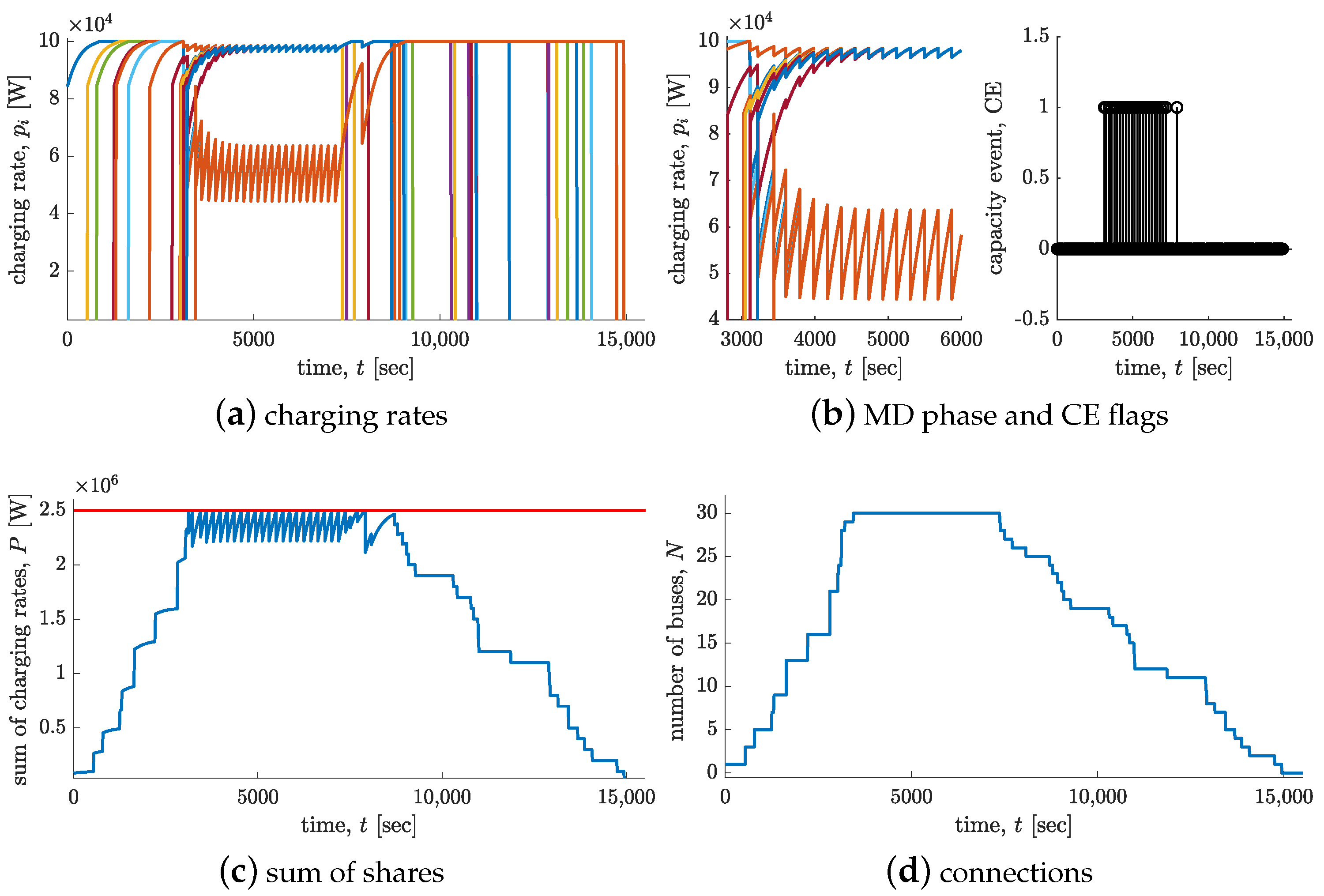
5.1. Case Study 1: Charging Rate Allocation of an Existing Plant

This case explores the effectiveness of the proposed charging strategy based on an existing plant in Milan city. The maximum power of the considered plant is $2.5$ $\mathrm{M}$$\mathrm{W}$, and the related charging depot is able to charge up to $N=30$ electric buses after their daily service time.

Table 1. Scenario settings and outcomes in terms of charging times.

Bus i	${\underline{\mathit{t}}}_{\mathit{i}}$ (s)	${\mathit{E}}_{\mathit{i}}\left({\underline{\mathit{t}}}_{\mathit{i}}\right)$ (kW h)	${\overline{\mathit{t}}}_{\mathit{i}}-{\underline{\mathit{t}}}_{\mathit{i}}$ (h min)	${\overline{\mathit{t}}}_{\mathit{i}}$ (h min)
1	1	34.14	3 h 18${}^{\prime }$	3 h 18${}^{\prime }$
2	538	5.6	3 h 35${}^{\prime }$	3 h 44${}^{\prime }$
3	538	109.11	1 h 59${}^{\prime }$	2 h 8${}^{\prime }$
4	784	85.93	2 h 47${}^{\prime }$	3 h
5	784	124.737	1 h 50${}^{\prime }$	2 h 3${}^{\prime }$
6	1252	90.47	2 h 10${}^{\prime }$	2 h 31${}^{\prime }$
7	1252	118.51	1 h 54${}^{\prime }$	2 h 14${}^{\prime }$
8	1311	102.58	2 h 3${}^{\prime }$	2 h 25${}^{\prime }$
9	1311	100.27	2 h 4${}^{\prime }$	2 h 26${}^{\prime }$
10	1637	148.54	1 h 35${}^{\prime }$	2 h 3${}^{\prime }$
11	1637	145.03	1 h 38${}^{\prime }$	1 h 5${}^{\prime }$
12	1637	24.04	3 h 24${}^{\prime }$	3 h 52${}^{\prime }$
13	1637	50.82	3 h 28${}^{\prime }$	3 h 36${}^{\prime }$
14	2218	66.62	2 h 59${}^{\prime }$	3 h 36${}^{\prime }$
15	2218	45.24	3 h 12${}^{\prime }$	3 h 49${}^{\prime }$
16	2218	121.80	1 h 52${}^{\prime }$	2 h 29${}^{\prime }$
17	2809	76.50	2 h 53${}^{\prime }$	3 h 40${}^{\prime }$
18	2809	82.67	2 h 49${}^{\prime }$	3 h 18${}^{\prime }$
19	2809	68.85	2 h 57${}^{\prime }$	3 h 44${}^{\prime }$
20	2809	50.66	3 h 8${}^{\prime }$	3 h 55${}^{\prime }$
21	2809	87.33	2 h 14${}^{\prime }$	3 h 1${}^{\prime }$
22	3023	141.22	1 h 40${}^{\prime }$	2 h 30${}^{\prime }$
23	3023	32.51	3 h 19${}^{\prime }$	4 h 10${}^{\prime }$
24	3049	103.74	2 h 3${}^{\prime }$	2 h 53${}^{\prime }$
25	3117	108.50	1 h 59${}^{\prime }$	2 h 55${}^{\prime }$
26	3117	137.10	1 h 43${}^{\prime }$	2 h 38${}^{\prime }$
27	3117	89.24	2 h 11${}^{\prime }$	3 h 7${}^{\prime }$
28	3117	89.70	2 h 11${}^{\prime }$	3 h 6${}^{\prime }$
29	3215	92.32	2 h 9${}^{\prime }$	2 h 3${}^{\prime }$
30	3441	44.60	3 h 9${}^{\prime }$	4 h 6${}^{\prime }$

reports the arrival time and the corresponding residual energy for each vehicle in the considered scenario. The batteries of the vehicles are identical and have the characteristic curves illustrated in Figure 2, with a capacity of 304 $\mathrm{k}$$\mathrm{W}$$\mathrm{h}$, initial charge level between 0 $\mathrm{k}$$\mathrm{W}$$\mathrm{h}$ and 150 $\mathrm{k}$$\mathrm{W}$$\mathrm{h}$ (see Table 1) and maximum charging rate equal to 100 $\mathrm{k}$$\mathrm{W}$. Finally, as for the NAIMD algorithm and the mechanism (23), the decrease factors ${\beta }_i$ with $i=1,\dots ,N$ are selected such that ${\beta }^{\left(1\right)}$ = 0.7 and ${\beta }^{\left(2\right)}=0.98$.

Figure 4 shows the outcomes in terms of charging rates, total power, capacity events and number of connected buses. As expected, when the sum of shares is smaller than $\overline{P}=2.5 \mathrm{M}\mathrm{W}$, the charging rates increase up to the saturation ${\overline{p}}_i=100 \mathrm{k}\mathrm{W}$ following the characteristic curve of the batteries (CE flag equal to zero). Then, when the sum of the charging rates is equal to the capacity $\overline{P}=2.5 \mathrm{M}\mathrm{W}$, a CE takes place (CE flag equal to 1) and each share instantaneously decreases (see, e.g., the close up of the MD phase in Figure 4) according to its decrease factor selected as in (23). Moreover, whenever a bus is fully charged and is disconnected from the spot, the associated charging rate is set to zero.

In Table 1, the duration of the charging process for each vehicle and the final time computed from the first connection time instant are also reported. It can be noticed that the last bus ($i=23$) is charged after 4 h and 10 min, while the average charging time is 2 h and 30 min.

Having in mind the field implementation of the proposal, consider now the case of different saturation limits and reduced power capacities of the plant. Indeed, the EMS can decide to reduce the power limits of some batteries for safety reasons, due to, for instance, the overheating of their components. Moreover, for economical and efficiency reasons, the maximum power of the plant can be also reduced. Therefore, consider ${\overline{p}}_i\in \{50,75,100\}$$\mathrm{k}\mathrm{W}$, as well as three different values of the maximum capacity, i.e., $\overline{P}\in \{1,1.5,2\}\mathrm{M}\mathrm{W}$.

The outcomes are shown in Figure 5, where the time evolution of the charging rate of each user and the CE flags are illustrated for $\overline{P}\in \{1,1.5,2\}\mathrm{M}\mathrm{W}$, respectively. As expected, the duration of the charging process increases as the maximum capacity $\overline{P}$ decreases, and as a consequence, the number of CEs—that is, the communications from the EMS—is much greater.

Furthermore, in order to deeply analyze the obtained charging times, for each value of $\overline{P}$, 50 simulations with different initial charging conditions randomly generated have been performed.

Table 2. Average of charging times and process duration for $\overline{P}\in \{1,1.5,2\}\mathrm{M}\mathrm{W}$ over 50 simulations.

$\overline{\mathit{P}}$ (MW)	${\mathit{\mu }}_{\mathbf{ct}}$ (h min)	${\mathit{\mu }}_{\mathbf{dc}}$ (h min)
1	5 h 11′	9 h 44′
1.5	3 h 55′	7 h 50′
2	3 h 26′	7 h 1′

reports the average values of the charging times, namely ${\mu }_{\mathrm{ct}}$, and of the duration of the total charging process, ${\mu }_{\mathrm{dc}}$. By reducing the maximum available power, the average charging time increases, and the charging rates reach the maximum capacity in a time interval that is shorter when $\overline{P}$ is smaller, with also a greater number of CEs. These considerations pave the way for exploiting the proposed approach to suitably size a charging plant in progress, as discussed in the following.

5.2. Case Study 2: Sizing of a Bus Charging Plant

Motivated by the previous case study, now, the problem of finding the minimum adequate grid capacity $\overline{P}$ while satisfying predefined constraints on the charging times is considered. The used data and parameters refer to a plant in progress in Alessandria, Italy.

The daily service window (gray slots) and the charging window (white slots) associated with a real fleet of buses are reported in

Table 3. Time slots for the considered charging plant with service time (gray slots) and allowed charging window (white slots) for each bus.

Bus i	09:00 10:00	10:00 11:00	11:00 12:00	12:00 13:00	13:00 14:00	14:00 15:00	15:00 16:00	16:00 17:00	17:00 18:00	18:00 19:00	19:00 20:00	20:00 21:00	21:00 22:00	22:00 23:00	23:00 24:00	24:00 01:00	01:00 02:00	02:00 03:00	03:00 04:00	04:00 05:00	05:00 06:00	06:00 07:00	07:00 08:00	08:00 09:00
1
2
3
4
5
6
7
8
9
10
11
12
13
14
15
16
17
18
19
20
21
22
23
24
25
26
27
28
29
30
31
32
33
34
35
36
37
38
39
40
41
42
43
44
45
46
47
48
49
50

.

Moreover, it is assumed that each bus arrives at the depot and is immediately connected to its charging spot. If the charging process of a bus ends before the related charging time slot, that bus has to wait for starting its service. The bus fleet consists of 50 vehicles, whose batteries are of the same type considered in the previous scenario, with two different saturation levels, i.e., ${\overline{p}}_i\in \{50,100\}$. As for the energy request, in the available data of the scenario, the batteries, which have a very limited time available for charging, have high initial autonomy. Based on this consideration, batteries, which have only one hour to be recharged, have initial energy autonomy equal to $50\%$ of maximum capacity. Batteries with two, three and four hours available for charging have an initial energy capacity equal to $40\%$, $30\%$ and $20\%$ of the maximum one, respectively. Finally, batteries that have at least five hours to complete their charging process have an initial energy level equal to $10\%$ of the maximum capacity. In addition, it is requested to disconnect vehicles from the charging spots whenever the $90\%$ of the maximum energy capacity is reached so as to preserve the life of batteries. As for the adopted NAIMD algorithm, the decrease factors ${\beta }^{\left(1\right)}$ and ${\beta }^{\left(2\right)}$, selected according to (23), are chosen equal to ${\beta }^{\left(1\right)}$ = 0.7 and ${\beta }^{\left(2\right)}=0.98$, while the best size of the plant has to be selected among three levels—that is, $\overline{P}\in \{1,1.5,2\}$$\mathrm{M}\mathrm{W}$.

Figure 6 shows the time evolution of the charging rates, and the corresponding sum of shares in the case of the three different levels of $\overline{P}$. It can be observed that the reduction of the whole capacity implies an increase in the CEs, as already highlighted in the previous case study. As a consequence, the sum of charging times tends to increase as well. More precisely, the case $\overline{P}=1 \mathrm{M}\mathrm{W}$ is the most critical since some constraints on the pre-specified charging intervals are violated. Therefore, comparing the other two cases—that is $\overline{P}=1.5 \mathrm{M}\mathrm{W}$ and $\overline{P}=2 \mathrm{M}\mathrm{W}$—in terms of sum of charging times (see

Table 4. Sum of charging times J and number of CEs in the case of $\overline{P}\in \{1,1.5,2\}$$\mathrm{M}\mathrm{W}$.

$\overline{\mathit{P}}$$\left(\mathbf{MW}\right)$	J (h)	# CEs
1	346.77	491
1.5	226.52	74
2	195.12	12

), although the first one can be a good compromise for economical and efficiency reasons, the best solution is given by the second one. In fact, it guarantees shorter charging times and a reduced amount of communication due to the smaller number of CEs.

6. Concluding Remarks

In this paper, an innovative approach for the charging of electrical bus fleets has been designed relying on the so-called AIMD resource allocation strategy. Therefore, taking into account the nonlinear nature of the charging process dynamics, on the basis of real data, the battery model has been recast in the framework of an NAIMD method. More precisely, the so-called decrease phase of the NAIMD algorithms has been designed in order to enable the minimization of the sum of charging times of all the electric buses, without requiring full knowledge of the state of charge of each vehicle. In fact, each bus requires only partial and aggregated information on the energy request of the other vehicles, while the maximum power availability is monitored by the central SCADA unit in order to generate the CEs to enable the decrease phase of the shares. Relying on the real case studies considered in this work, the actual SCADA architectures are able to provide such information, thus making the proposed approach a promising ready-to-implement solution for future charging plants.

Moreover, the wide simulation campaign has shown the potentiality of the NAIMD algorithm in field implementation and its capacity to address the charging problem in the case of multiple vehicles contemporarily connected to the grid in the presence of a limited power resource. Finally, given the considerable advantages in terms of scalability and communication bandwidth, the proposed NAIMD approach can be also used to size real plants given stricter constraints in terms of charging times and saturation powers of each electric vehicle. Indeed, another important aspect is the electricity cost associated with the charging processes. It typically consists of variable and fixed costs. While the variable ones depend on the energy consumption during charging, the fixed costs strictly depend on the power capacity of the plant and on the communication network needed to fulfil the information required by the control strategy. As a consequence, the proposal has the potential to be particularly adequate for massively large-scale distributed settings, and because of the small amount of needed information, it is preferable to other solutions.

Future work will be devoted to the development of alternative AIMD solutions, even of the nonsynchronized type, to take into account different recharging priorities of the vehicles, directly including additional control objectives such as the minimization of power losses and the maximization of the operation profits.

References

1. Sneha Angeline, P.; Newlin Rajkumar, M. Evolution of electric vehicle and its future scope. Mater. Today Proc. 2020, 33, 3930–3936. [Google Scholar] [CrossRef]
2. Deb, S.; Tammi, K.; Kalita, K.; Mahanta, P. Impact of Electric Vehicle Charging Station Load on Distribution Network. Energies 2018, 11, 178. [Google Scholar] [CrossRef] [Green Version]
3. Ouramdane, O.; Elbouchikhi, E.; Amirat, Y.; Sedgh Gooya, E. Optimal Sizing and Energy Management of Microgrids with Vehicle-to-Grid Technology: A Critical Review and Future Trends. Energies 2021, 14, 4166. [Google Scholar] [CrossRef]
4. Hassler, J.; Dimitrova, Z.; Petit, M.; Dessante, P. Optimization and Coordination of Electric Vehicle Charging Process for Long-Distance Trips. Energies 2021, 14, 4054. [Google Scholar] [CrossRef]
5. Ding, X.; Zhang, W.; Wei, S.; Wang, Z. Optimization of an Energy Storage System for Electric Bus Fast-Charging Station. Energies 2021, 14, 4143. [Google Scholar] [CrossRef]
6. Zhou, K.; Cheng, L.; Wen, L.; Lu, X.; Ding, T. A coordinated charging scheduling method for electric vehicles considering different charging demands. Energy 2020, 213. [Google Scholar] [CrossRef]
7. Apostolaki-Iosifidou, E.; Codani, P.; Kempton, W. Measurement of power loss during electric vehicle charging and discharging. Energy 2017, 127, 730–742. [Google Scholar] [CrossRef]
8. Wang, S.; Bi, S.; Zhang, Y.J.A.; Huang, J. Electrical Vehicle Charging Station Profit Maximization: Admission, Pricing, and Online Scheduling. IEEE Trans. Sustain. Energy 2018, 9, 1722–1731. [Google Scholar] [CrossRef] [Green Version]
9. Tan, J.; Wang, L. Real-Time Charging Navigation of Electric Vehicles to Fast Charging Stations: A Hierarchical Game Approach. IEEE Trans. Smart Grid 2017, 8, 846–856. [Google Scholar] [CrossRef]
10. Xu, S.; Yan, Z.; Feng, D.; Zhao, X. Decentralized charging control strategy of the electric vehicle aggregator based on augmented Lagrangian method. Int. J. Electr. Power Energy Syst. 2019, 104, 673–679. [Google Scholar] [CrossRef]
11. Zhang, K.; Xu, L.; Ouyang, M.; Wang, H.; Lu, L.; Li, J.; Li, Z. Optimal decentralized valley-filling charging strategy for electric vehicles. Energy Convers. Manag. 2014, 78, 537–550. [Google Scholar] [CrossRef]
12. Zhan, K.; Hu, Z.; Song, Y.; Lu, N.; Xu, Z.; Jia, L. A probability transition matrix based decentralized electric vehicle charging method for load valley filling. Electr. Power Syst. Res. 2015, 125, 1–7. [Google Scholar] [CrossRef]
13. Ireshika, M.A.S.T.; Lliuyacc-Blas, R.; Kepplinger, P. Voltage-Based Droop Control of Electric Vehicles in Distribution Grids under Different Charging Power Levels. Energies 2021, 14, 3905. [Google Scholar] [CrossRef]
14. Li, S.; Hu, W.; Cao, D.; Dragičević, T.; Huang, Q.; Chen, Z.; Blaabjerg, F. Electric Vehicle Charging Management Based on Deep Reinforcement Learning. J. Modern Power Syst. Clean Energy 2021, 1–12. [Google Scholar] [CrossRef]
15. Corless, M.; King, C.; Shorten, R.; Wirth, F. AIMD Dynamics and Distributed Resource Allocation; SIAM: Philadelphia, PA, USA, 2016; Volume 29. [Google Scholar]
16. Stuedli, S.; Corless, M.; Middleton, R.; Shorten, R. On the AIMD Algorithm Under Saturation Constraints. IEEE Trans. Autom. Control 2017, 62, 6392–6398. [Google Scholar] [CrossRef]
17. Studli, S.; Crisostomi, E.; Middleton, R.; Shorten, R. A flexible distributed framework for realising electric and plug-in hybrid vehicle charging policies. Int. J. Control 2012, 85, 1130–1145. [Google Scholar] [CrossRef]
18. Studli, S.; Crisostomi, E.; Middleton, R.; Shorten, R. Optimal real-time distributed V2G and G2V management of electric vehicles. Int. J. Control 2014, 87, 1153–1162. [Google Scholar] [CrossRef]
19. Crisostomi, E.; Shorten, R.; Studli, S.; Wirth, F. Electric and Plug-in Hybrid Vehicle Networks: Optimization and Control; CRC Press: Boca Raton, FL, USA, 2017. [Google Scholar]
20. Nisar Shah, S.; Incremona, G.P.; Bolzern, P.; Colaneri, P. Optimization based AIMD saturated algorithms for public charging of electric vehicles. Eur. J. Control 2019, 47, 74–83. [Google Scholar] [CrossRef]
21. Moschella, M.; Murad, M.A.A.; Crisostomi, E.; Milano, F. Decentralized Charging of Plug-In Electric Vehicles and Impact on Transmission System Dynamics. IEEE Trans. Smart Grid 2021, 12, 1772–1781. [Google Scholar] [CrossRef]
22. Ravasio, M. Optimization AIMD Algorithms for a Real Electric Bus Charging Plant. Master’s Thesis, Politecnico di Milano, Milan, Italy, 2020. [Google Scholar]
23. Chiu, D.M.; Jain, R. Analysis of the Increase and Decrease Algorithms for Congestion Avoidance in Computer Networks. Comput. Netw. Isdn Syst. 1989, 17, 1–14. [Google Scholar] [CrossRef] [Green Version]
24. Pozzi, A.; Torchio, M.; Braatz, R.D.; Raimondo, D.M. Optimal charging of an electric vehicle battery pack: A real-time sensitivity-based model predictive control approach. J. Power Sources 2020, 461, 228133. [Google Scholar] [CrossRef]
25. Houbbadi, A.; Trigui, R.; Pelissier, S.; Redondo-Iglesias, E.; Bouton, T. Optimal Scheduling to Manage an Electric Bus Fleet Overnight Charging. Energies 2019, 12, 2727. [Google Scholar] [CrossRef] [Green Version]
26. Liu, Z.; Song, Z.; He, Y. Planning of Fast-Charging Stations for a Battery Electric Bus System under Energy Consumption Uncertainty. Transp. Res. Rec. 2018, 2672, 96–107. [Google Scholar] [CrossRef] [Green Version]
Figure 1. Charging of electric buses. (a) Example of an electric bus. (b) Charging spot realization. (c) Electric scheme of the plant.
Energies 14 04389 g001
Figure 2. Characteristic curves of the batteries. (a) Current–voltage curve. (b) Power–voltage curve. (c) Current ι i over time. (d) Power p i over time. (e) Voltage v i over time. (f) SOC over time.
Energies 14 04389 g002
Figure 3. Scheme of the considered NAIMD-based architecture with four buses.
Energies 14 04389 g003
Figure 4. Simulation results when P ¯ = 2.5   M W and all the batteries have saturation equal to p ¯ i = 100   k W . (a) Time evolution of charging rates. (b) Close up of the MD phase and CEs over time. (c) Sum of shares and total capacity. (d) Time evolution of the number of connected buses to be recharged.
Energies 14 04389 g004
Figure 5. Simulation results in terms of charging rates and CEs when p ¯ i { 50 , 75 , 100 } k W , and the maximum capacity assumes values P ¯ { 1 , 1.5 , 2 } M W .
Energies 14 04389 g005
Figure 6. Simulation results in terms of charging rates and sum of shares in the case of P ¯ { 1 , 1.5 , 2 } M W and charging time slots as in Table 3.
Energies 14 04389 g006