Abstract
The paper presents a new method for modelling the warming up process of a water system with elements regulating the flow in a stochastic manner. The paper presents the basic equations describing the work of typical elements which the water installation is composed of. In the proposed method, a new computational algorithm was used in the form of an iterative procedure enabling the use of boundary conditions that can be stochastically modified during the warming-up process. A typical situation, when such a modification is processed, is the regulation of the medium flow through two-way or three-way valves or applying additional heat source. Moreover, the presented method does not require the transformation of the differential equations, describing the operation of individual elements, into a linear form, which significantly facilitates analytical work and makes it more flexible. The example of analysis of the operation of water installation used for controlling temperature of the process gases in a chemical installation shows the functionality and flexibility of the method. The adopted calculation schematics enable changing the direction of the heat flow while the heat exchanger is in operation. Additionally, the sequence of calculation processed in modules describing operation of installation elements is elective (there is no situation that output parameters from one element are used as input parameters for other element in the same calculation step).
1. Introduction
The problems of dynamics of heating and cooling process in elements of heat and mass transfer matter practically in district heating, [1,2], cooling and air-conditioning systems [3,4,5,6], electronics, chemical systems [7,8] and in devices where unsteady heat transfer is a standard operating mode, e.g., Stirling engines [9,10]. In terms of the correct functioning of the above-mentioned installations [11], it is important to ensure the effective cooperation of the heat and mass transport elements with the regulating elements [12,13,14,15]. The quality of cooperation can be determined by numerical simulation, using efficient models and a flexible interface [16,17,18,19] enabling the correct implementation of the installation into the computing environment, as well as definition of boundary and initial conditions [20,21].
In commonly used methods of modelling water installation warming-up processes, it is expected that modelled energy system is described by a certain number of equations concerning the laws of conservation: mass, energy and momentum with simultaneously defined boundary conditions. The set of differential equations obtained from the analysis is usually non-linear and should be reduced to linear form so that it is possible to use standard numerical methods to solve them [22].
In detail, two methods are employed for solving the problem described above: one is an algebraic approach and the other one is differential [22]. Models derived using the algebraic approach assume that either the system operates at steady-state or the transient response does not significantly impact the outcome of the analysis [23,24]. The model is then used simultaneously for optimization of the construction and parameters of operation, e.g., rate of flow or temperatures in the system [25]. Differential approach for modelling of water installation warming-up process can grasp the dynamic response of the system, but it requires numerical solution of the problem described by nonlinear differential equations. In this approach, the temperatures are considered as searched variables in the analyzed points of the system [26].
Another approach is the application of heat transmission matrices describing the linear relation between the temperature and the power of the two sides of a heat-transmitting component [27,28].
An analysis of heat transfer process dynamics with the application of an equivalent electric circuit model has also been applied [29].
Modelled heat exchange systems can be divided into control elements related to other heat transport mechanisms, e.g., in a proton exchange membrane fuel cell, the first control element is an anode and a cathode, while the second control element is the liquid in the cooling channels [22]. Heat accumulation can then be considered independently in these two control elements. For the simulation of the warming-up or cooling process of such systems, the average temperature of the fluid in the exchanger channels is taken into account, its rate of change is defined by the rate of stored energy [30]. The average fluid temperature is calculated on the basis of the inlet and outlet temperature of the analyzed device [22,31]. The heat flux received in the membrane heat exchanger, also under dynamic conditions, is calculated using lumped parameters based on the average wall temperature, average fluid temperature and the total heat exchange surface [9,22]. This approach facilitates the calculations but makes it impossible to take into account the nonlinear distribution of wall and fluid temperature inside the heat exchanger. This approach, in the case of proton exchange membrane fuel cell modelling, micro-combined heat and power system, made it possible to map the temperatures in the analyzed points having a maximum root mean square error of 2.38 °C over an operating range of approximately 30–60 °C.
When calculating the warming-up or cooling-down process of the heat accumulator, it is also assumed that the analyzed area can be divided into several control spaces, however, this division is going in the horizontal direction, due to the stratification of the deposit temperature which follows the direction of change in the density of the deposit. The lowest density and the highest temperature is on the top of the heat accumulator [22]. Then, the analysis of the temperature change process is also carried out for the lumped parameters, assuming that one control volume has the same temperature. The calculations take into account both the process of heat accumulation in a single control volume, as well as the heat exchange between the walls and adjacent control volumes [22,32]. Hot water tanks are also considered as constant temperature heat sources [33].
In the case of elements joining or dividing heat fluxes, it is assumed that these elements are well insulated and heat losses can be neglected. On the other hand, the fluid temperature and mass flow rate at the outlet are calculated on the basis of the first law of energy balance and the conservation of mass [22,34].
The propagation of water in pipes can be modelled by considering the inlet and outlet of a pipe and calculating the output based on the propagation delay [35,36].
The paper presents a new method for modelling the warming-up process of a water system with elements regulating the flow in a stochastic manner. The paper presents the basic equations describing the work of typical elements which the water installation is composed of. The installation is used to control the temperature of chemical reactors which can be used in petrochemical processes like methanol synthesis and synthetic gas production [37]. In commonly used methods, the modelling of the warming-up process of such systems is performed by solving the conservation equations describing the operation of individual elements of the installation, with clearly defined boundary conditions. In the proposed method, a new computational algorithm was used in the form of an iterative procedure, enabling the use of boundary conditions that can be stochastically modified during the warming-up process. A typical situation, when such a modification is processed, is the regulation of the medium flow through two-way or three-way valves or applying an additional heat source, e.g., a heat storage tank. Moreover, the presented method does not require the transformation of the differential equations describing the operation of individual elements into a linear form, which significantly facilitates analytical work and makes it more flexible. The paper presents an example of modelling the warming-up process of a water installation controlling the operation of chemical reactors typically used in industry.
2. Modelling the Operation of Water System Elements
2.1. Heat Exchanger
One of the key elements of temperature control in chemical installations is gas–liquid cooling or heating medium. In the considered approach, the heat exchanger is defined as a system delivering heat to the water from the gas or delivering the heat in opposite direction (it is not necessary to define the direction of heat flow), with the possibility of heat accumulation in the water and the membrane separating gas from water. Due to the relatively low heat capacity of the gas in such a heat exchanger as compared with the heat capacity of the membrane and water, the share of gas in the heat storage process has been neglected [38]. A schematic drawing of a heat exchanger with a heat accumulator in the membrane and the cooling medium has been shown in Figure 1.
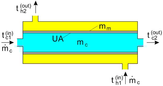
Figure 1.
Schematic drawing of a heat exchanger with a heat accumulator in the membrane and the cooling medium.
For the system shown in Figure 1, the following equation describing the energy balance can be assumed, neglecting the losses to the environment:
where Qin is heat flux delivered by the cooling medium, QUA is heat flux transferred between heating and cooling medium, Qout is the heat flux discharged by the cooling medium and Qacc is the heat flux delivered to the heat accumulating elements.
where is mass flow rate of the cooling medium in the heat exchanger, cc is specific heat of the cooling medium, tc1 is inlet temperature of the cooling medium.
where U is the overall heat transfer coefficient, A is heat transfer surface, –logarithmic temperature difference.
where tc2 is outlet temperature of the cooling medium.
where mc is the mass of the coolant in the heat exchanger, is the mass of the heat-conducting membrane in the heat exchanger, is the specific heat of the heat-conducting membrane in the heat exchanger, is an increase in the average temperature of the cooling medium over time ∆τ, and ∆τ is the time step of calculations.
where th1 is inlet temperature of the heating medium, and th2 is the outlet temperature of the heating medium.
It was assumed that the change in the average temperature of heat-accumulating elements over time ∆τ can be determined on the basis of the average temperature of the cooling medium between the inlet and the outlet of the heat exchanger. It was assumed that the temperature values of the heat-conducting membrane and the cooling medium are the same due to the large difference in the specific heat of the cooling and heating medium (water–gas) on the other side of the heat-conducting membrane:
where is the average temperature of the cooling medium in the heat exchanger during the previous calculation step, and is the average temperature of the cooling medium in the heat exchanger in the current calculation step.
where τ is a current time of the process.
By the discretization of the process of the operation of the installation, the current time of the process can be replaced by calculation steps (k):
The average temperature of the cooling medium in the heat exchanger in the previous (ini) and current (end) calculation steps can then be defined as follows:
At the same time, the condition that the heat flux transferred between heating and cooling medium must be equal to the heat flux change in the heating medium must be met:
where is the mass flow rate of the heating medium, th1 is the inlet temperature of the heating medium, and th2 is the outlet temperature of the heating medium.
Solving the above set of equations is analytically difficult due to their non-linear nature. Therefore, in this paper a new method of problem solving, based on an iterative procedure, has been proposed. The layout of the heat exchanger module has been presented in Figure 2.
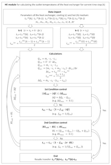
Figure 2.
Layout of the heat exchanger module.
2.2. Three-Way Equal Joint
In a three-way equal joint, it is possible to mix two fluids of different temperatures or to separate a fluid into two streams of the same temperature. In the considered case, the first of the mentioned variants will be analyzed. In Figure 3, a schematic of a three-way equal joint used to combine two streams of fluids of different temperatures has been shown.
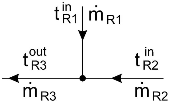
Figure 3.
Schematic drawing of a three-way equal joint used to combine two streams of fluids of different temperatures.
For this system, neglecting the heat losses to the surroundings, the energy balance can be presented as an equation:
where is the heat flux in a pipeline „i”.
is the mass flow rate in a pipeline „i”, cc is the specific heat of the cooling medium, and is the inlet fluid temperature „i”
where is the outlet fluid temperature „i”.
where is the mass flow rate in a pipeline „i”,
Using energy balance, it is possible to calculate the outlet temperature in a three-way equal joint:
2.3. Controlled Two-Way Valve
A controlled two-way valve is used to regulate the pressure and flow rate through the pipeline. Any throttling element, e.g., nozzle, filter, can also be computationally treated in this way. The scheme of the controlled two-way valve is shown in Figure 4.
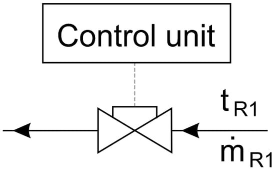
Figure 4.
Schematic drawing of a controlled two-way valve.
In the model of the controlled two-way valve, the temperature on the inlet and outlet of the element is assumed to be the same, but the flow rate can be calculated according to the following equation:
where is f2V is a fraction of mass flow rate through the two-way valve to the maximum mass flow rate for that valve, is maximum mass flow rate in pipeline.
2.4. Controlled Three-Way Valve
In a controlled three-way valve, it is possible, similarly to the three-way equal joint, to combine two fluid streams or to separate them (Figure 5). Below, the analysis of a variant related to combining two fluid streams of different temperatures with the controller which can smoothly adjust the share of mass flow of fluids from the input pipelines has been presented. On the basis of the energy balance for this system, it is possible to calculate the temperature of the fluid in the outlet pipeline, while the mass flow rate of the fluid in one of the pipelines can be defined on the basis of the proportion set by the controller:
and
where f3V is the fraction of mass flow rate in the first (inlet) pipeline to the mass flow rate in the outlet pipeline of a three-way valve.
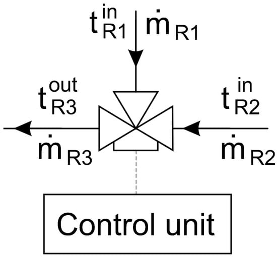
Figure 5.
Schematic drawing of a controlled three-way valve to combine two streams of fluids of different temperatures.
2.5. Pipeline
The section of the pipeline delivering fluid to the fittings has a volume that directly affects the delay in heat transport between the nodes of the system, e.g., between the heating element and the cooler (Figure 6). If the heat losses to the surroundings are neglected, it can be assumed that the impulse of the temperature change reaches from the beginning to the end of the pipeline in the following time:
where is a temperature impulse delay time in the pipeline, is the average density of the cooling medium in the pipeline, VR is the volume of the analyzed pipeline, and is the mass flow rate of the cooling medium in the pipeline
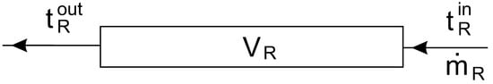
Figure 6.
Schematic drawing of a pipeline section.
However, the temperature impulse delay time can be calculated as the number of calculation steps that will elapse between the triggering of the impulse at the entrance to the pipeline and the impulse reaching the outlet from the pipeline:
The outlet temperature can be then calculated using the following relation:
Or
where is the inlet temperature of a cooling medium entering the pipeline for calculation step (k), is the outlet temperature of a cooling medium leaving the pipeline for calculation step (k), and is the initial outlet temperature of a cooling medium leaving the pipeline.
3. Modular Model for Computing Operation of a Water Installation with Elements Regulating the Flow
Each element of the installation is represented by one module, which incorporates iterative procedure for solving equations describing the operation of the considered element. Calculations are processed independently in each module. The algorithm presented below enables the usage of boundary conditions that can be stochastically modified during the warming-up process. It is assumed that stochasticity of the control process results from the superior role of the controller. A layout of the modular model for computing operations of water installation with elements regulating the flow has been shown in Figure 7. In the demonstrated method, it was assumed that calculations have been conducted sequentially, for a selected process time (calculation steps), separated from each other by a constant time step ∆τ. The results of calculations from previous calculation step are used as initial conditions for the next calculation step. Calculations for subsequent elements of the installation such as: heat exchangers, joints, controlled valves and pipelines are lead periodically for each calculation step (indicated process time) in relevant modules. Because of the application of elements causing a response delay in the form of pipeline sections between connected elements of installation, the sequence of calculations processed in modules describing the operation of installation elements is elective (there is no situation that output parameters from one element are used as input parameters for the other element in the same calculation step).
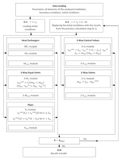
Figure 7.
Layout of the modular model for computing operation of the water installation with elements regulating the flow.
The original element of the method is application of elements controlled in a stochastic manner, which can receive a control signal, based on any strategy, also modified during the installation operation; it does not affect the order of calculations and does not require modification of the calculation algorithm. In the proposed calculation method, in the module describing the operation of the heat exchanger, an original solution was also used to calculate the temperatures of the fluids outgoing the heat exchanger through the use of two conditional loops. The first loop controls the condition that the amount of energy received by the metal membrane is equal to the amount of energy given by the hot fluid, this condition is described by Equation (15). The second loop, the external one, is used to control the condition that the amount of energy balance within the heat exchanger is maintained (1), also taking into account the processes of energy accumulation. Such a two-stage control of the conditions of maintaining energy balances in the exchanger enables the use of equations in its original form, e.g., the logarithmic temperature difference (6), and the result of the procedure operation is to determine the values of two variables in parallel, in this case the temperatures of fluids leaving the heat exchanger. This is a significant simplification in relation to the commonly used iterative methods, where there is one loop enabling the determination of one variable. Moreover, it was assumed that the mass of the exchanger metal membrane and the fluid in the heat exchanger have the same temperatures due to the large difference in the heat capacity of the fluids on both sides of the heat-conducting membrane. In the applications considered below, one fluid is a water and the other one is a process gas, the heat capacity ratio in this case is reaching 1000. The adopted calculation schematics enable calculations to be made both for the heat flow from the heating fluid to the cooling fluid, as well as in the opposite direction. It is also possible to change the direction of the heat flow while the heat exchanger is in operation. It is possible due to using conditional definition of the temperature difference in the heat exchanger (6). Depending on the temperatures of the fluid at the inlet and outlet, the definition of the temperature difference adopts proper notation to avoid mathematically forbidden actions, e.g., division by zero.
4. Analysis of the Warming up Process of the Water System
In Figure 8, a schematic of the water installation used for cooling or heating the process gases of a chemical installation has been shown. The installation consists of four heat exchangers for heating or cooling the process gases (W1–W4), a cooler (C1), a water pump, four adjustable three-way valves, an expansion tank and 16 selected pipeline sections (R1–R16). In exchangers W1–W3, heat is delivered by the process gases, while in the heat exchanger W4 the process gas is heated. The operation of the cooler (C1) has not been analyzed; this element has a thermal performance twice the maximum demand and, in combination with the control system, transfers any excess heat to the surroundings. Table 1 describes the parameters of the installation and the initial conditions.
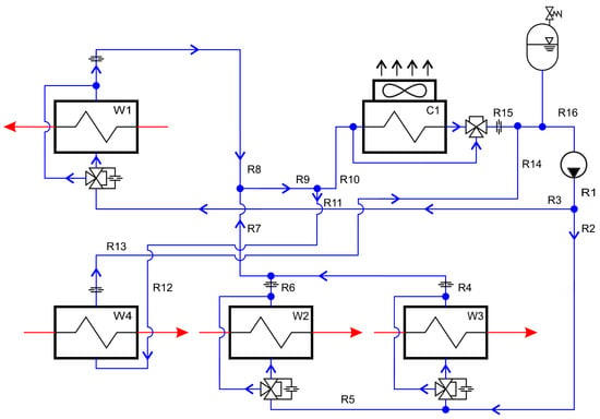
Figure 8.
Schematic drawing of the water installation used for controlling the temperature of the process gases in the chemical installation.

Table 1.
Parameters of the analyzed installation and the initial conditions (constant).
In the analysis, it has been assumed that the temperatures of the process gases at the inlet to the heat exchangers are constant, also during the start-up of the installation. On the other hand, the water temperature in the system, during start-up, is the same in all points of the installation. Taking into account the volumes of pipelines and heat exchangers, the warming-up of the system does not have a uniform course. Impulse of water temperature change is reaching the end of the pipeline with delay depending on length of the pipeline and the mas flow rate. This effect can be observed in pipelines R7 and R15 (Figure 9), the presented temperatures refer to the parameters at the outlet. Figure 9 shows the moment when the controller decides to activate the cooler C1 and pass a part of the water stream from the pipeline R10 through the cooler, and some through the bypass, in such a share that the temperature at the outlet from the pipeline R15 is 110 °C. This temperature is then maintained by the controller until the end of the analyzed operation of the installation.
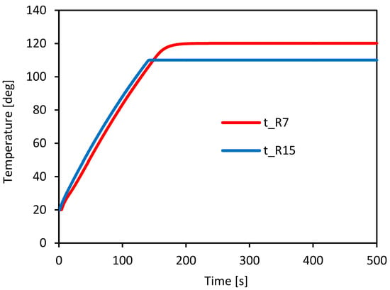
Figure 9.
Outlet temperature of pipeline R7 and R15.
Figure 10, Figure 11 and Figure 12 show the warming-up process of the heat exchangers W1–W3, calculated with the use of the algorithm described in Figure 7. The heat exchanger warming-up process takes about 200 s. After its completion, the water temperature at the outlet has a constant temperature, also the process’ gas maintains a constant temperature. The process of warming-up of the heat exchanger W4 has been shown in Figure 13. In this device, the inflowing water is used to warm-up the process gas.
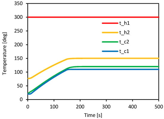
Figure 10.
Warming up process of the heat exchanger W1.
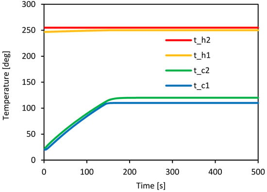
Figure 11.
Warming up process of the heat exchanger W2.
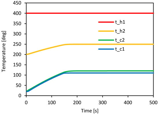
Figure 12.
Warming up process of the heat exchanger W3.
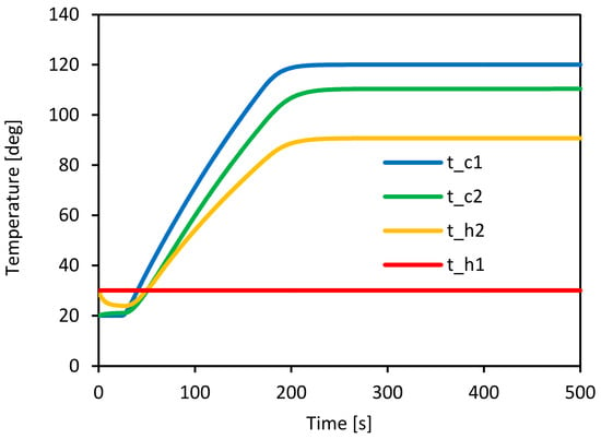
Figure 13.
Warming up process of the heat exchanger W4.
In the initial warming-up phase, the water has a lower temperature than the process gas, so that the heat flows in the opposite direction as initially designed. The application of the calculation algorithm presented in Figure 2 enables such a two-way heat flow analysis.
The analysis shows that the system is working stably and maintains the assumed temperature of the process gas after the warming-up process is completed (Figure 9, Figure 10, Figure 11, Figure 12 and Figure 13). The ratio of the heat capacity of the heat exchanger (metal membrane and water included) to the heat flux delivered is crucial for the warming-up time. On the basis of the presented results, it can be seen that the heat exchanger W4 (Figure 13), supplied with a relatively small heat flux, is warming-up the slowest, and in order to shorten this time, the heat flux should be increased or the heat exchanger mass should be reduced. The ratio of the water velocity in the pipeline to the water mass in the pipeline has a noticeable effect on the course of the heat exchanger warming-up process. This factor introduces a significant delay in the warming-up process, which can be clearly observed in the initial phase of the system operation in Figure 13. The delay resulting from the flow of water supplying the heat exchanger W4 is in this case as much as 26 s.
The verification of the results presented in Figure 9, Figure 10, Figure 11, Figure 12 and Figure 13 was carried out with the use of analytical methods. In the first stage, the model was verified for the steady state, and then for the warming-up state. For the system shown in Figure 8, calculations were made for the steady state using the energy conservation equations for heat exchangers W1–W4: (1)–(6), (15), (16), and the boundary conditions were formulated on the basis of the results presented in Figure 9, Figure 10, Figure 11, Figure 12 and Figure 13 for the last operating point (500 s). In Table 2, a comparison of water temperatures at the outlet of heat exchangers W1–W4, for the steady state, have been shown.
Table 2.
Water outlet temperature comparison for steady state.
For the model verification purposes during the warming-up, the system shown in Figure 8 has been reduced to one equivalent heat exchanger composed of one cumulated metal mass (25.46 kg), while the water mass in the equivalent heat exchanger is the sum of the water masses in all heat exchangers and pipelines (48.80 kg). The heat flux supplied to the equivalent heat exchanger is the average value of the sum of heat fluxes supplied in individual heat exchangers (96.96 kW). Table 3 shows a comparison of the warming-up time of the W1–W4 heat exchangers calculated with the use of the numerical model shown in Figure 7 and with the use of an equivalent heat exchanger (verification system).
Table 3.
Comparison of the warming-up time of heat exchangers W1-W4 calculated with the use of a numerical model and an equivalent heat exchanger (verification system).
Based on the obtained results, it can be concluded that the presented model with high accuracy reflects the operating conditions of the system in the steady state and during the warming-up process, the shorter warming-up time obtained during the verification results from the use of the constant value of the heat flux, which is calculated as the arithmetic mean for the initial and the final state. In practice, the heat flux present in the initial phase of the warming-up process is going down very quickly. This happens because of rapid reduction of the logarithmic temperature difference. That causes the real average heat flux for the warming-up process is lower than that adopted during the verification, and the real warming-up time is longer.
The above analysis was carried out for an iterative time step amounting to 1 s. Figure 14 shows the effect of iterative time step on the water temperature leaving the heat exchanger W4. However, in all analyzed cases, the convergence control is performed with the use of the condition that the left and right side of the energy balance in the heat exchanger (1) cannot differ from each other by more than 0.1 J.
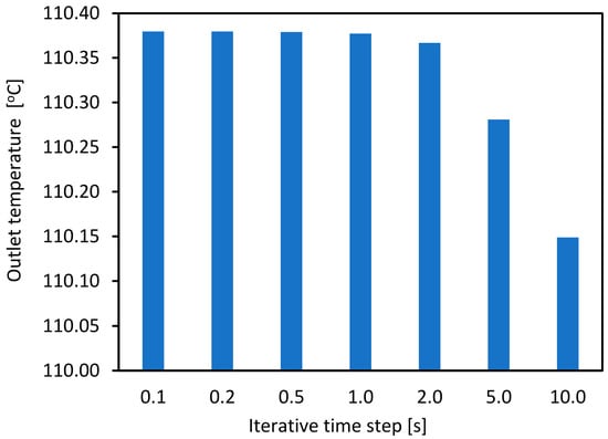
Figure 14.
Effect of iterative time step on the water temperature leaving the heat exchanger W4.
The presented data show that an iterative time step of 1 second or less practically does not affect the calculated value of the water temperature leaving the heat exchanger W4. On the other hand, for the iterative time step of 2 s and more, this effect becomes visible, and the difference in the calculated value of the water temperature leaving the heat exchanger W4 slightly exceeds 0.2 °C. Due to the very short calculation time achieved on a standard personal computer (less than 1 s), it was concluded there is no need to use a smaller iterative time step than one second.
5. Conclusions
The paper presents a new method for modelling the warming-up process of a water system with elements regulating the flow in a stochastic manner. The controller is responsible for the stochastic way of regulating the fluid flow through the system elements. The controller makes decisions based on the expected process gases temperatures. In addition, the controller may take into account the chemical process control algorithm (expected heating or cooling rate) or the adopted technological restrictions in the form of permissible extreme temperatures or pressures.
The main advantage of the proposed method is the modular construction of the model. Additional installation modules can be added and subtracted from the model in a very easy way, it is possible due to application of the iterative calculation method. The results from the previous calculation step are the initial conditions for the next calculation step. Calculations can be carried out parallel (independently) in all modules. Moreover, the presented method does not require the transformation of the differential equations describing the operation of individual elements into a linear form, which significantly facilitates the analytical work and makes it more flexible. For example, when calculating the temperatures of the cooled and heated medium at the outflow of the heat exchanger, the equations describing operation of the element have been left in its original form in the algorithm.
The paper presents calculation algorithms for the basic elements of the water system, such as heat exchangers, three-way controlled valves, two-way controlled valves (throttling elements), joints and pipeline sections. The example of the analysis of operation of water installation used for controlling temperature of the process gases in the chemical installation shows the functionality and flexibility of the method. The obtained results make it possible to assess the correctness of operation of the control system governing process gases temperatures, from the moment the cooling water reaches the temperature of 110 °C. The proposed model of the installation enables also assessing the correctness of operation of the control system in the event of simulated disturbances in the course of chemical processes, e.g., changes in the mass flow rate of the process gas or its temperature.
Author Contributions
Conceptualization, J.K.; Investigation, M.F.; Methodology, J.K.; Resources, A.R.; Validation, M.F. and A.R.; Writing—original draft, J.K. All authors have read and agreed to the published version of the manuscript.
Funding
This research was co-founded by National Centre of Research and Development and PGNiG SA (Polskie Górnictwo Naftowe i Gazownictwo SA) in the EU Smart Growth Operational Programme, grant number POIR.04.01.01-00-0064/18-00.
Institutional Review Board Statement
Not applicable.
Informed Consent Statement
Not applicable.
Data Availability Statement
Data is contained within the article.
Conflicts of Interest
The authors declare no conflict of interest.
Abbreviation
| Index | |
| A | heat transfer surface [m2], |
| cc | specific heat of the cooling medium [J/(kg·K)], |
| ch | specific heat of heating medium [J/(kg·K)], |
| cm | specific heat of the heat-conducting membrane in the heat exchanger [J/(kg·K)], |
| f2V | fraction of mass flow rate through the two-way valve to the maximum mass flow rate for that valve [-], |
| f3V | fraction of mass flow rate in the first (inlet) pipeline to the mass flow rate in the outlet pipeline of a three-way valve [-] |
| k | number of step calculation [-], |
| kR | number of calculation steps that will elapse between the triggering of the impulse at the entrance to the pipeline and the impulse reaching the outlet from the pipeline [-], |
| mc | mass of the cooling medium in the heat exchanger [kg], |
| mass of the heat-conducting membrane in the heat exchanger [kg], | |
| mass flow rate of the cooling medium [kg/s] | |
| mass flow rate of the heating medium [kg/s] | |
| maximum mass flow rate in pipeline ,,i’’ [kg/s], | |
| average temperature of the cooling medium in the heat exchanger during the current calculation step [s], | |
| average temperature of the cooling medium in the heat exchanger during the previous calculation step [s], | |
| tc1 | inlet temperature of cooling medium [K], |
| tc2 | outlet temperature of cooling medium [K],, |
| th1 | inlet temperature of heating medium [K], |
| th2 | outlet temperature of heating medium [K], |
| inlet temperature in pipeline ,,i” [K] | |
| inlet temperature of a cooling medium entering the pipeline for calculation step (k) [K] | |
| outlet temperature in pipeline ,,i” [K] | |
| outlet temperature of a cooling medium leaving the pipeline for calculation step (k) [K], | |
| initial outlet temperature of a cooling medium leaving the pipeline [K], | |
| Qacc | heat flux delivered to the heat accumulating elements [W] |
| Qin | heat flux delivered with the cooling medium, |
| Qout | heat flux discharged by the cooling medium [W], |
| heat flux in pipeline „i” [W], | |
| QUA | heat flux transferred between heating and cooling medium [W], |
| U | overall heat transfer coefficient [W/(m2·K)], |
| VR | volume of the analyzed pipeline [m3]. |
| Greek symbols | |
| ∆Qh | heat flux change in the heating medium, |
| ∆tav | increase in the average temperature of the cooling medium over time ∆τ [K/s] |
| logarithmic temperature difference [K], | |
| ∆τ | time step of calculations [s], |
| average density of the cooling medium in the pipeline [kg/m3] | |
| temperature impulse delay time in pipeline [s] | |
| Subcripts | |
| ini | previous calculation step, |
| end | current calculation step. |
References
- Van der Heijde, B.; Fuchs, M.; Tugores, R.; Schweiger, G.; Sartor, K.; Basciotti, D.; Müller, D.; Nytsch-Geusen, C.; Wetter, M.; Helsen, L. Dynamic equation-based thermo-hydraulic pipe model for district heating and cooling systems. Energy Convers. Manag. 2017, 151, 158–169. [Google Scholar] [CrossRef]
- Lund, H.; Werner, S.; Wiltshire, R.; Svendsen, S.; Eric, J.; Hvelplund, F. 4th Generation district heating (4GDH) integrating smart thermal grids into future sustainable energy systems. Energy 2014, 68, 1–11. [Google Scholar] [CrossRef]
- Buffa, S.; Cozzini, M.; D’Antoni, M.; Baratieri, M.; Fedrizzi, R. 5th generation district heating and cooling systems: A review of existing cases in Europe. Renew. Sustain. Energy Rev. 2019, 104, 504–522. [Google Scholar] [CrossRef]
- del Hoyo Arce, I.; Herrero López, S.; López Perez, S.; Rämä, M.; Klobut, K.; Febres, J.A. Models for fast modelling of district heating and cooling networks. Renew. Sustain. Energy Rev. 2018, 82, 1863–1873. [Google Scholar] [CrossRef]
- Ndiaye, D. Reliability and performance of direct-expansion ground-coupled heat pump systems: Issues and possible solutions. Renew Sustain. Energy Rev. 2016, 66, 802–814. [Google Scholar] [CrossRef]
- Wang, X.; Ma, C.; Lu, Y. An experimental study of a direct expansion ground-coupled heat pump system in heating mode. Int. J. Energy Res. 2009, 33, 1367–1383. [Google Scholar] [CrossRef]
- Bieniasz, L.K.; Bureau, C. Use of dynamically adaptive grid techniques for the solution of electrochemical kinetic equations: Part 7. Testing of the finite difference patch-adaptive strategy on example kinetic models with moving reaction fronts, in one-dimensional space geometry. J. Electroanal. Chem. 2000, 481, 152–167. [Google Scholar] [CrossRef]
- Wysocka, I.; Mielewczyk-Gryń, A.; Łapiński, M.; Cieślik, B.; Rogala, A. Effect of small quantities of potassium promoter and steam on the catalytic properties of nickel catalysts in dry/combined methane reforming. Int. J. Hydrog. Energy 2021, 46, 3847–3864. [Google Scholar] [CrossRef]
- Ulloa, C.; Miguez, J.L.; Porteiro, J.; Egula, P.; Cacabelos, A. Development of a Transient Model of a Stirling-based CHP System. Energies 2013, 6, 3115–3133. [Google Scholar] [CrossRef]
- Kropiwnicki, J.; Furmanek, M. A Theoretical and Experimental Study of Moderate Temperature Alfa Type Stirling Engines. Energies 2020, 13, 1622. [Google Scholar] [CrossRef]
- El Azab, H.-A.I.; Swief, R.A.; El-Amary, N.H.; Temraz, H.K. Unit Commitment Towards Decarbonized Network Facing Fixed and Stochastic Resources Applying Water Cycle Optimization. Energies 2018, 11, 1140. [Google Scholar] [CrossRef]
- Skoglund, T.; Årzén, K.E.; Dejmek, P. Dynamic object-oriented heat exchanger models for simulation of fluid property transitions. Int. J. Heat Mass Transf. 2006, 49, 2291–2303. [Google Scholar] [CrossRef]
- Wajs, J.; Gołąbek, A.; Bochniak, R.; Mikielewicz, D. Air-cooled photovoltaic roof tile as an example of the BIPVT system – An experimental study on the energy and exergy performance. Energy 2020, 197, 117255. [Google Scholar] [CrossRef]
- Dehghan, A.A.; Barzegar, A. Thermal performance behaviour of a domestic hot water solar storage tank during consumption operation. Energy Convers. Manag. 2011, 52, 468–476. [Google Scholar] [CrossRef]
- Kamal, R.; Moloney, F.; Wickramaratne, C.; Narasimhan, A.; Goswami, D.Y. Strategic control and cost optimization of thermal energy storage in buildings using EnergyPlus. Appl. Energy 2019, 246, 77.e90. [Google Scholar] [CrossRef]
- Dahash, A.; Mieck, S.; Ochs, F.; Krautz, H.J. A comparative study of two simulation tools for the technical feasibility in terms of modelling district heating systems: An optimization case study. Simul. Model. Pr. Theory 2019, 91, 48–68. [Google Scholar] [CrossRef]
- Li, D.; Wang, J.; Ding, Y.; Yao, H.; Huang, Y. Dynamic thermal management for industrial waste heat recovery based on phase change material thermal storage. Appl. Energy 2019, 236, 1168–1182. [Google Scholar] [CrossRef]
- Kuang, J.; Zhang, C.; Li, F.; Sun, B. Dynamic optimization of combined cooling, heating, and power systems with energy storage units. Energies 2018, 11, 2288. [Google Scholar] [CrossRef]
- Li, P.; Wang, H.; Lv, Q.; Li, W. Combined Heat and Power Dispatch Considering Heat Storage of Both Buildings and Pipelines in District Heating System for Wind Power Integration. Energies 2017, 10, 893. [Google Scholar] [CrossRef]
- Oppelt, T.; Urbaneck, T.; Gross, U.; Platzer, B. Dynamic thermo-hydraulic model of district cooling networks. Appl. Therm. Eng. 2016, 102, 336–345. [Google Scholar] [CrossRef]
- Giraud, L.; Merabet, M.; Baviere, R.; Vallée, M. Optimal control of district heating systems using dynamic simulation and mixed integer linear programming. In Proceedings of the 12th International Modelica Conference, Prague, Czech Republic, 15–17 March 2017; pp. 141–150. [Google Scholar]
- Bird, T.J.; Jain, N. Dynamic modelling and validation of a micro-combined heat and power system with integrated thermal energy storage. Appl. Energy 2020, 271, 114955. [Google Scholar] [CrossRef]
- Arsalis, A.; Nielsen, M.P.; Kær, S.K. Modelling and optimization of a 1 kWe HT-PEMFC based micro-CHP residential system. Int. J. Hydrog. Energy 2012, 37, 2470–2481. [Google Scholar] [CrossRef]
- Van der Heijde, B.; Aertgeerts, A.; Helsen, L. Modelling steady-state thermal behaviour of double thermal network pipes. Int. J. Therm. Sci. 2017, 117, 316–327. [Google Scholar] [CrossRef]
- Adam, A.; Fraga, E.S.; Brett, D.J.L. A modelling study for the integration of a PEMFC micro-CHP in domestic building services design. Appl. Energy 2018, 225, 85–97. [Google Scholar] [CrossRef]
- König, P.; Weber, A.; Lewald, N.; Aicher, T.; Jörissen, L.; Ivers-Tiffée, E. Model-aided testing of a PEMFC CHP system. Fuel Cells 2007, 7, 70–77. [Google Scholar] [CrossRef]
- Gori, P.; Guattari, C.; de Lieto Vollaro, R.; Evangelisti, L. Accuracy of lumped-parameter representations for heat conduction modelling in multilayer slabs. J. Phys. Conf. 2015, 655, 012065. [Google Scholar] [CrossRef]
- Bácsi, Á. The number of independent elements in heat transmission matrices. Int. J. Therm. Sci. 2019, 138, 496–503. [Google Scholar] [CrossRef]
- Bianco, G.; Bracco, S.; Delfino, F.; Gambelli, L.; Robba, M.; Rossi, M. A Building Energy Management System Based on an Equivalent Electric Circuit Model. Energies 2020, 13, 1689. [Google Scholar] [CrossRef]
- Li, Y.; Wenjie, X.; Ling, M.; Zhao, J.; Wenjia, L.; Shihe, W.; Jiulong, L. Dynamic heat transfer analysis of a direct-expansion CO2 downhole heat exchanger. Appl. Therm. Eng. 2021, 189, 116733. [Google Scholar] [CrossRef]
- Jung, W.; Kim, D.; Ha Kang, B.; Soo Chang, Y. Investigation of Heat Pump Operation Strategies with Thermal Storage in Heating Conditions. Energies 2017, 10, 2020. [Google Scholar] [CrossRef]
- Powell, K.M.; Edgar, T.F. An adaptive-grid model for dynamic simulation of thermocline thermal energy storage systems. Energy Convers. Manag. 2013, 76, 865–873. [Google Scholar] [CrossRef]
- Giménez, S.N.; Durá, J.M.H.; Ferragud, F.X.B.; Fernández, R.S. Control-oriented modeling of the cooling process of a PEMFC-based μ-CHP system. IEEE Access 2019, 7, 95620–95642. [Google Scholar] [CrossRef]
- Barone, G.; Buonomano, A.; Forzano, C.; Palombo, A. A novel dynamic simulation model for the thermo-economic analysis and optimisation of district heating systems. Energy Convers. Manag. 2020, 220, 113052. [Google Scholar] [CrossRef]
- Vesterlund, M.; Dahl, J. A method for the simulation and optimization of district heating systems with meshed networks. Energy Convers. Manag. 2015, 89, 555–567. [Google Scholar] [CrossRef]
- Gabrielaitiene, I.; Bøhm, B.; Sunden, B. Modelling temperature dynamics of a district heating system in Naestved, Denmark–a case study. Energy Convers. Manag. 2007, 48, 78–86. [Google Scholar] [CrossRef]
- Wysocka, I.; Hupka, J.; Rogala, A. Catalytic activity of nickel and ruthenium–Nickel catalysts supported on SiO2, ZrO2, Al2O3, and MgAl2O4 in a dry reforming process. Catalysts 2019, 9, 540. [Google Scholar] [CrossRef]
- Cichy, M.; Kropiwnicki, J.; Kneba, Z. A Model of Thermal Energy Storage According to the Convention of Bond Graphs (BG) and State Equations (SE). Pol. Marit. Res. 2015, 22, 41–47. [Google Scholar] [CrossRef]


Publisher’s Note: MDPI stays neutral with regard to jurisdictional claims in published maps and institutional affiliations. |
© 2021 by the authors. Licensee MDPI, Basel, Switzerland. This article is an open access article distributed under the terms and conditions of the Creative Commons Attribution (CC BY) license (https://creativecommons.org/licenses/by/4.0/).