Numerical Investigation on the Urban Heat Island Effect by Using a Porous Media Model

Abstract

The urban heat island (UHI) effect resulted from urbanization as well as industrialization has become a major environmental problem. UHI effect aggravates global warming and endangers human health. Thus, mitigating the UHI effect has become a primary task to address these challenges. This paper verifies the feasibility of a three-dimensional turbulent porous media model. Using this model, the authors simulate the urban canopy wind-heat environment. The temperature and flow field over a city with a concentric circular structure are presented. The impact of three factors (i.e., anthropogenic heat, ambient crosswind speed, and porosity in the central area) on turbulent flow and heat transfer in the central business district of a simplified city model with a concentric circular structure were analyzed. It is found that the three-dimensional turbulent porous media model is suitable for estimating the UHI effect. The UHI effect could be mitigated by reducing the artificial heat and improving the porosity of the central city area.

1. Introduction

With global urbanization increasing, the rapid change in the structure of modern cities (e.g., high-density buildings) and human activities’ increasing (e.g., heavy urban traffic) have made urban heat islands (UHI) more and more serious. [1]. The UHI intensity can increase rapidly with the city size and a maximum intensity of 12 K was observed in Lodz (Poland) and Mexico City (Mexico) [2]. Environmental problems in cities (i.e., reduced diffusion capacity of waste heat and pollution) have become the primary concern for city dwellers.

Manley first proposed the concept of the UHI in 1958 [3]. Currently, it has been generally accepted that UHI is a climatic phenomenon with higher temperature in towns and lower temperature in suburbs. Since the concept was proposed, many scholars have investigated UHI phenomena using field measurement methods, such as meteorological data and fixed-point, mobile, and infrared thermal measurements. Mathew and Kaul [4] analyzed the surface temperature data of the Chandigarh study area from 2009 to 2013 and found that a significant surface heat island phenomenon existed in the area. The UHI intensity of the targeted area changed with the seasons. Huang et al. [5] selected four types of land cover for microclimate research in Nanjing and analyzed the characteristics of the Nanjing heat island using temperature data from four fixed observation points. Sun et al. [6] conducted both mobile observations and fixed-point measurements to investigate the UHI effect. Sabiha and Satyanarayana [7] quantified the spatial relationships among the land occupations, planting and ground temperatures of 10 major metropolitan cities in India using satellite remote sensing and messaging systems. It was difficult to describe the spatial structure of UHIs with limited data obtained from field measurements. Singhe et al. [8] analyzed the data collected by satellites to study land occupation, planting and land temperature and their impact on surface temperature. The results show that urbanization has a greater impact on the distribution of surface temperature with computing power improving, an increasing number of studies have been published investigating urban climate issues using numerical simulations and mesoscale and microscale climate models [9]. Khan and Simpson [10] established a mesoscale model to study the UHI effect in Brisbane using local meteorological data. The results showed that additional heat sources affected the temperature field of the city during breezes. Atkinson [11] established a three-dimensional numerical model of the UHI in London and analyzed various factors affecting the UHI. Takahashi et al. [12] measured the temperatures of commercial buildings, university campuses, plaza buildings, and street surfaces in Tokyo in the summer of 2002 and established a prediction model. The results showed that the model could predict the urban thermal environment. Yushkov et al. [13] applied the mesoscale weather research and forecasting (WRF) model to describe the mixing process of the atmospheric boundary layer in detail and concluded that the model could only capture the main features of UHIs. Vitanova and Kusaka [14] investigated the characteristics of UHI and found that the degree of urbanization’s intensification impacted urban temperature distribution Mirzaei and Haghighat [9] reviewed the mathematical models for the study of UHIs. They found that the methods for the modeling of UHI were not sound. Mesoscale models were typically used in computational fluid dynamics (CFD) simulations to describe urban heat conduction. However, they had low horizontal accuracy, usually within the range of several kilometers. It was also difficult to describe the aerodynamic characteristics and thermal effects in the urban canopy. In contrast, microscale models could accurately depict the geometric features and architectural details of a city. However, it was extremely challenging to apply a microscale model to an entire city. Computational grids were not sufficient to model the building sizes, and the existing computing power cannot handle a large number of computational grids required for city-scale CFD simulations. Hang and Li [15] pointed out that the minimum grid resolution should be 10% of the building scale to simulate urban areas using the Reynolds-averaged Navier–Stokes (RANS) turbulence model. Thousands of buildings in urban require billions of grids, which cannot be handled by conventional CFD models.

Porous medium is defined as the material composed of solid substance and small gaps separated by a large number of densely spaced pores. Porous media can be divided into primary porous media and secondary porous media. Building materials such as bricks and wood are secondary porous media. It was observed that the urban spatial structure and porous media were very similar in terms of the topological structure. Therefore, cities are secondary porous media. Therefore, Hang and Li [15] approximated the urban space as a porous medium consisting of solid buildings and the spaces between the buildings and the used volume averaging. Although some micro-information in the simulated urban area was ignored in volume averaging, it could still simulate the impact of building clusters on urban airflow accurately. The Darcy term (Darcy Law means the groundwater movement throughout pores and fractures. This refers to the resistance of airflow in the pores), Forchheimer term, and Brinkman term in the momentum equation were used to describe the drag force generated by the buildings and the underlying surface. The application of an urban porous media model can significantly simplify the numerical model, facilitating urban-scale modeling.

Parker et al. earlier proposed a porous media parameter model. [16]. Since then, many scholars have performed macroscale flow experiments and numerical simulations of porous media [17,18,19]. Some researchers have conducted in-depth analyses of the mathematical equations of flow in porous media as well as proposed various modifications of Darcy’s law according to the physical properties of flow [20]. Whitaker et al. [21] derived the Forchheimer correction of Darcy’s law for uniform porous method adopting the volume averaging technology. The macro turbulence method based on porous media was continuously improved in the literature. Antohe and Lage [22] established and derived a two-equation turbulence model of incompressible flow in saturated rigid porous media. Subsequently, several researchers modified this model to study the airflow in an urban canopy. Brown and Decroix [23] conducted a wind tunnel experiment on a set of cube buildings, providing data for subsequent CFD simulation validation. Lien et al. [24] conducted detailed microscale numerical simulations of airflow in comparable cube arrays. Meanwhile, they carried out a macroscale simulation with an improved turbulence model to study the macroscale dynamics of airflow in the cubic array with porous properties. Hang and Li [15] proposed for the first time that a city could be treated to be porous. The revised porous media model was adopted by Antohe and Lage [22] to study the macroscale flows in the city. These studies provide theoretical guidance and methodological references for our work. Hu et al. [25] derived an urban porous method to investigate the urban airflow and UHI phenomenon. Hang and Li [26] adopted the porous method to study spatially averaged macro wind conditions of urban high-rise areas. Wang et al. [27] proposed a hybrid model that considered some buildings in the city as a porous medium, whereas the target buildings had full resolution. They applied the revised porous turbulence model developed by Hang and Li [15] to simulate the entire city. The scale of the modeling domain was expanded without missing the important characteristics of airflow in the studied area, and the computing power was proven sufficient. Wang and Li [28] proposed a multiscale CFD model suitable for urban airflow prediction. The authors used the porous method to simulate the urban boundary layer and successfully applied the model to study urban heat island circulation (UHIC), which is considered a challenging issue in CFD. This study laid the foundation for our study of the UHI within a city. Yang et al. [29] treated plants as porous media to simulate the influence of vegetation on the flow field and pollutants in 2D urban street canyons. Fan et al. [30] used the existing porous turbulence model to simulate the urban canopy and studied the formation mechanism of buoyancy and turbulence-driven atmospheric circulation (BTDAC) with low-level inflow and reverse divergent outflow from external rural areas in the upper mixed layer. In recent years, some scholars have performed outdoor scale experimental measurements. Chen et al. [31] conducted outdoor measurements to study the effect of aspect ratio on flow and heat transmission on the street. Chen et al. [32] made a field experiment to study the effect of aspect ratios and building heat storage on urban heat transfer.

The two-dimensional turbulent porous media model has been adopted to research the UHI effect. However, research on the three-dimensional turbulent porous media model is lacking. The urban spatial form is a key factor affecting the UHI effect. Therefore, it is vital to demonstrate that the three-dimensional turbulent porous method is suitable to study the UHI effect. Gu and Zhang [33] used a three-dimensional turbulent porous media model to study airflow in Fengxi New City, which laid the foundation for future work and provided a method, references, and a theoretical basis for our work.

Cities have various shapes. In large cities with an approximately circular shape, the functional areas form a concentric structure. Chicago, Tokyo, Moscow, Paris, Chengdu, and Beijing are examples of large cities with circular shapes. Therefore, investigation for the UHI effect of the cities with a concentric structure is essential. This paper adopts a three-dimensional turbulent porous mothed to study the UHI effect of a small-scale city with a concentric circle structure. The research results provide a reference for alleviating the UHI problem of cities with this structure. The entire city was considered to be a secondary porosity porous media porous medium. The macroscale flow and heat transfer inside the city were modeled employing a turbulence porous media model. The effects of anthropogenic heat, building density, and ambient crosswind speed on the UHI of the city were investigated. The modeling results could be used to guide making scientific urban development plans to mitigate the UHI effect.

2. Model Descriptions and Methodology

2.1. Geometric Model

Burgess proposed a concentric structure model of an urban area and provided a graphical description [34]. The concentric circle model was divided into five concentric areas, i.e., the central business district, the transitional area, the workers’ residential area, the better-quality residential area, and the senior residential area, according to Burgess’ theory. The central business district was designed as a place for commerce, culture, and other major social activities, as well as the center of the urban transportation network. The transition zone was originally a residential area for the rich. Due to the continuous development of industry and commerce, it gradually became a place where environmental quality declined. In our paper, we simply refer to the three residential areas in the concentric circle model as residential areas. Cities with a concentric circle structure are generally clumpy structure cities. Only when the city’s area is relatively large and the shape is close to a circle, can each functional area form a ring structure. Urban flows have large spatial and temporal ranges. The urban scale in this study is in mesoscale (1–100 km) [35]. According to the pollutant dispersion theory, the studied area could be separated into five scales. The urban scale is 10–20 km [36].

Since real cities are complex and large scale, this paper establishes a three-dimensional physical model of the urban structure of a small-scale concentric circle model. Different building partitions with different building heights, building densities, and bottom heat flux densities are used. Due to the symmetry of the concentric circle model, the wind direction is not considered in this study as a factor influencing the UHI. The porosity, anthropogenic heat of the central business district, and the ambient crosswind speed are considered as influencing factors. As shown in Figure 1a, London is a city with a typical concentric circle pattern. To simplify the modeling (Figure 1b), the following assumptions are made: (1) The calculation domain size is 11,000 m (x) ×10,000 m (y) × 800 m (z). We use half of the domain in the calculation because the geometric model is symmetric to reduce the computing resources; (2) The urban area consists of three concentric circles, namely, the central area, the transition area, and the residential area from the inside to the outside of the circles. The heights of the areas are 80 m, 40 m, and 20 m, respectively. The diameters of the concentric circles are 1000 m, 3000 m, and 5000 m, respectively; (3) The entire city is treated as a porous area, and porosity is consistent in each area. The calculation domain includes the urban areas and the free flow field areas. The porosity of the free flow field area is 1.0, and that of the urban area is 0.6–0.8; (4) The physical properties of the transition zone and residential area are the same.

2.2. Mathematical Model

The surface-averaged ψ^v and volume-average ψ^f are typically used to describe the characteristics of porous media. Whitaker [21] defined two time-averaged values, $\overline{{\psi }^v}$ and $\overline{{\psi }^f}$, to describe turbulent flow in porous area. Macroscale time-averaged value was obtained by the microscale volume-averaged and time-averaged value for a basic representative volume. The macroscale time-averaged volume was calculated as follows:

$$\overline{{\psi }^v}=\frac{1}{\Delta V_v}{\displaystyle \underset{\Delta V_v}{\int }\overline{\psi }dV}$$

(1)

$$\overline{{\psi }^f}=\frac{1}{\Delta V_f}{\displaystyle \underset{\Delta V_f}{\int }\overline{\psi }dV}$$

(2)

$$\overline{{\psi }^v}=\varphi \overline{{\psi }^f}$$

(3)

where ΔV_v indicates total volume of basic representative volume. ΔV_f represents fluid volume of basic representative volume. In this paper, $\overline{{\psi }^v}$ and $\overline{{\psi }^f}$ are written as ψ^v, and ψ^f. The porosity $\varphi$ represents the volume fraction of the fluid, which is given by

$$\varphi ={\psi }^f/{\psi }^v$$

(4)

The airflow passing through the building arrays was set to be incompressible turbulent flow. The porous turbulence method was employed to study the airflow. Hang and Li [15] proposed a single domain method to determine the transport equation using macro k-ε porous media method derived by Antohe and Lage [22]. This equation provided an improved prediction of the velocity of the fluid flowing through the building arrays. The thermal properties were assumed to remain the same, except air density. The Coriolis force generated by the rotation of the earth was not considered. The transport equation of the porous media method was simplified as follows. The flow domain lower than the building altitude was referred to as urban canopy. Since maximum building altitude is typically less than 200 m, the compressible airflow in the urban canopy is usually ignored. The transport equation of the incompressible flow in the urban canopy was defined as follows:

Continuity equation:

$$\frac{\partial (\phi u_i^{\mathrm{f}})}{\partial x_i}=0$$

(5)

The momentum conservation equation:

$$\frac{\rho \partial (\phi u_i^{\mathrm{f}}{u}_j^{\mathrm{f}})}{\partial x_j}=\frac{\partial }{\partial x_j}\left[(\mu J+{\mu }_t)\frac{\partial \phi u_i^{\mathrm{f}}}{\partial x_j}\right]-(\frac{\partial \phi p^{\mathrm{f}}}{\partial x_i}+\frac{2}{3}\rho \frac{\partial \phi k^{\mathrm{f}}}{\partial x_i})$$

$$-\stackrel{\mathrm{udarcy}}{\overbrace{\phi \frac{\mu }{K}\phi u_i^{\mathrm{f}}}}-\stackrel{uForch}{\overbrace{\phi \frac{\rho C_F}{\sqrt{K}}\phi Q^{\mathrm{f}}\phi u_i^{\mathrm{f}}}}+{\delta }_{\mathrm{i}3}\rho \left[\beta \left(T-T_{in}\right)-1\right]$$

(6)

Equation for the turbulent kinetic energy (TKE):

$$\frac{\rho \partial (\phi u_i^{\mathrm{f}}{k}^{\mathrm{f}})}{\partial x_j}=\frac{\partial }{\partial x_j}\left[(\mu J+\frac{{\mu }_t}{{\sigma }_k})\frac{\partial \phi k^{\mathrm{f}}}{\partial x_j}\right]-\rho \phi {\epsilon }^{\mathrm{f}}+\stackrel{TKEgen}{\overbrace{\phi G_k}}\stackrel{TKEdarcy}{\overbrace{-2\phi \frac{{\mu }_{\mathrm{l}}}{K}\phi k^{\mathrm{f}}}}$$

$$\stackrel{TKEForch}{\overbrace{-\frac{8}{3}{\phi }^2\rho \frac{C_F}{\sqrt{K}}{Q}^{\mathrm{f}}\phi k^{\mathrm{f}}}}\stackrel{TKE\_FK}{\overbrace{+2\phi {\phi }^2\rho \frac{C_F}{\sqrt{K}}{F}_k}}$$

(7)

Equation for the energy dissipation:

$$\frac{\rho \partial (\phi u_i^{\mathrm{f}}{\epsilon }^{\mathrm{f}})}{\partial x_j}=\frac{\partial }{\partial x_j}\left[(\mu J+\frac{{\mu }_t}{{\sigma }_{\epsilon }})\frac{\partial \phi {\epsilon }^{\mathrm{f}}}{\partial x_j}\right]-C_{\epsilon 1}\phi \frac{{\epsilon }^{\mathrm{f}}}{k^{\mathrm{f}}}{G}_k-J\rho C_{\epsilon 2}\phi \frac{{\epsilon }^{\mathrm{f}}}{k^{\mathrm{f}}}{\epsilon }^{\mathrm{f}}$$

$$\stackrel{EDdarcy}{\overbrace{-2\phi \frac{{\mu }_{\mathrm{l}}}{K}\phi {\epsilon }^{\mathrm{f}}}}\stackrel{EDForch1}{\overbrace{-\frac{8}{3}{\phi }^3\rho \frac{C_F}{\sqrt{K}}{Q}^{\mathrm{f}}{\epsilon }^{\mathrm{f}}}}-\stackrel{EDForch2}{\overbrace{\frac{8\mu }{3}\varphi {\varphi }^2\frac{C_F}{\sqrt{K}}\frac{\partial k^f}{\partial x_r}\frac{\partial Q^f}{\partial x_r}}}$$

$$+\stackrel{EDForch3}{\overbrace{2{\varphi }^2\varphi \frac{C_F}{\sqrt{K}}\left[\mu v_t\frac{\partial }{\partial x_r}(\frac{u_j^{\mathrm{f}}{u}_i^{\mathrm{f}}}{Q^f})\frac{{\partial }^2{u}_i^{\mathrm{f}}}{\partial x_r\partial x_j}+2\mu v_t\frac{u_j^{\mathrm{f}}{u}_i^{\mathrm{f}}}{Q^f}\frac{{\partial }^2}{\partial x_r{}^2}(\frac{\partial u_i^{\mathrm{f}}}{\partial x_j})\right]}}$$

(8)

$$F_k={\mu }_{\mathrm{t}}\frac{u_i^{\mathrm{f}}{u}_j^{\mathrm{f}}}{Q^{\mathrm{f}}}\frac{\partial \phi u_j^{\mathrm{f}}}{\partial x_i}$$

(9)

$$G_k={\mu }_{\mathrm{t}}\frac{\partial u_i^{\mathrm{f}}}{\partial x_j}(\frac{\partial u_i^{\mathrm{f}}}{\partial x_j}+\frac{\partial u_j^{\mathrm{f}}}{\partial x_j})$$

(10)

$$Q=\sqrt{u_i{u}_i}$$

(11)

$${\mu }_{\mathrm{t}}=C_{\mu }\rho \frac{{(k^{\mathrm{f}})}^2}{{\epsilon }^{\mathrm{f}}}$$

(12)

ρ is fluid density; $u_i^{\mathrm{f}}$, $Q^{\mathrm{f}}$, $p^{\mathrm{f}}$, $k^{\mathrm{f}}$, and ${\epsilon }^{\mathrm{f}}$ represent the fluid velocity, intrinsic average velocity, pressure, turbulent kinetic energy, and turbulent dissipation rate. μ and μ_t are dynamic viscosity and turbulent viscosity, respectively. J is turbulent viscosity ratio, which was assumed to be 1 in porous media. σ_k, σ_ε, and C_μ are constants, with values of 1.0, 1.3, and 0.09. K and C_F are permeability and the Forchheimer coefficient, respectively, which were calculated as follows:

$$K=\frac{{\varphi }^3{h}^2}{150{(1-\varphi )}^2}$$

(13)

$$C_F=\frac{1.75\beta }{\sqrt{150{\phi }^3}}$$

(14)

where h is feature scale of the solid matter in the porous medium. β is the Constant, which is β = 1 in original Ergun equation.

In momentum equation (Equation (6)) and the TKE equation (Equation (7)), the Darcy terms (udarcy and TKEdarcy) and Forchheimer terms (uForch and TKEForch) indicates the viscous resistance of fluids and solids to fluids, respectively. These four terms have negative values, reflecting the reduction in the momentum and turbulent transport due to the Darcy force and Forchheimer force. In Equation (7), TKE_Fk is the second term of the TKE generated by the Forchheimer term, which is a sink or source term, depending on magnitude of velocity component. In Equation (8), Darcy source and first Forchheimer source are negative terms, resulting in turbulent dissipation. A comparative analysis of the above items was conducted by Hang and Li [15], who found that the Forchheimer term was larger than Darcy term by two magnitudes because the dynamic viscosity effect was relatively small in a flow with a high Reynolds number. It is assumed that EDForch2 and EDForch3 are much lower than EDForch1; thus, EDForch2 and EDForch3 are ignored in this study.

Buildings release artificial heat and radiant heat absorbed from the sun. Therefore, local heating cannot be used in the urban porous media model to describe heat exchange between buildings and air. Two equations are needed to describe the energy equations of the solid phase and the fluid phase. However, we only focused on the air temperature of the external flow field when studying the UHI, thus, we only considered the energy equation of the fluid phase. The heat transmission from building to air is regarded as the energy source term applied to the air region. The energy equation is defined as follows:

$$\frac{\partial (\rho c_p\varphi u_{j}T)}{\partial x_j}=\frac{\partial }{\partial x_j}(\lambda \varphi \frac{\partial T}{\partial x_j})+(1-\varphi )q$$

(15)

Urban heat sources mainly are waste heat generated by buildings and industries and ground heat sources. The surface heat source is expressed by distributing the heat flow on the ground surface. For building heat source, the heat source intensity per unit building volume (W/m³) q of the building was calculated by using Equations (16) and (17), which is the ratio of building intensity heat source per unit surface $Q_b$ (W/m²) to body surface area ratio $V_b$.

$$q=Q_b/V_b$$

(16)

The body surface area ratio is given by

$$V_b={\displaystyle \underset{0}{\overset{H}{\int }}(1-\varphi )}\mathrm{dz}$$

(17)

H is building altitude (m). In this paper, porosity is regarded as a constant in different areas of the porous medium, thus

$$V_b=\left(1-\phi \right)H$$

(18)

when the heat flux density of the bottom boundary is given. It is necessary to consider the influence of many factors on the absorption of solar radiation.

Reflection, scattering, and absorption of solar radiation by atmosphere and reflection by the ground surface weaken the solar radiation absorbed by the ground. Thus, solar radiation absorbed by the ground is approximately one-third of the incoming solar radiation. In addition, solar radiation entering the atmosphere is affected by the reflection and scattering of clouds. Zuev et al. [37] used statistical models to calculate the atmospheric absorption in the presence of clouds. The results showed that the cloud type and cloud cover affected the total absorption of the atmosphere. Martinez-Chico et al. [38] analyzed the temporal and spatial distribution of solar radiation under different weather conditions. The results showed that cloud types and characteristics are important factors for solar radiation attenuation. In addition, the albedo of different materials on the urban ground, the scattering and absorption of aerosols, and the absorption of water vapor also affect the solar radiation reaching the ground. In a simulation study of the UHI effect, the heat flux of the city was typically 100 W/m²–200 W/m² [39]. This study focuses on the effect of artificial heat on the UHI effect. Therefore, the evening period (100 W/m²) was chosen to study the effect of artificial heat on the UHI effect to reduce the influence of solar radiation.

2.3. Boundary Conditions

The vertical wind is influenced not only by weather but also by the thermal effect caused by the surface properties and terrain. Therefore, the wind speed changes with the altitude (see Figure 1b). An exponential or logarithmic function can be used for describing wind speed profile for inlet boundary conditions [40,41]. We used an exponential function in this study. Since the state of outlet flow is fully developed, the outlet boundary conditions are categorized as an outflow. Non-slip wall boundaries are set for building walls surfaces. The upper boundary of the building walls is defined to be symmetric. The side of the area is relatively far from the urban area. Thus, a symmetric plane is used.

The exponential function formula of gradient wind is as follows:

$$u_{in}=u_{ref}{(\frac{z}{z_{ref}})}^{0.16}$$

(19)

According to Li [15], the TKE and dissipation rate at the entrance are marked as follows:

$$k_{in}=0.01u_{ref}^2$$

(20)

$${\epsilon }_{in}=C_{\mu }{}^{3/4}{k}_{in}{}^{3/2}/(kz)$$

(21)

u_ref is the characteristic velocity at the altitude z_ref 20 m above the ground, and $\kappa$ is an empirical constant called the Von Karman constant which is 0.4.

The inlet temperature distribution along the height is as follows

$$T_{in}=T_0-\gamma z$$

(22)

where γ is the vertical temperature reduction rate (K∙m⁻¹).

The inlet pressure distribution along the height is

$$p_{in}=p_0-\rho gz$$

(23)

As shown in Figure 1b, the domain consists of a porous area and a transparent fluid area. The mass, kinetic energy, as well as turbulent exchange at the interface are complex. A single domain is used to resolve e complex interface issue. The computational domain is considered a porous medium. The clear fluid region is regarded as a porous area and its porosity is 1.0. Permeability K in the domain is infinite, and the Forchheimer term is close to 0. Thus, the turbulent transport equation of porous area is reduced to the general turbulent transport equation in clear fluid region.

2.4. Grid Independence Test and Computational Procedure

The grid quality of the structured grid is relatively high, with rapid convergence, and low computational requirements [42]. For the same meshing zone, a structured mesh is more economically and efficiently reduces false diffusion than an unstructured mesh. Therefore, a structured mesh was used in the calculation domain in this study. Figure 2 shows the grid in the entire computational domain and local grid size in the city porous medium area. The grid size in the porous area should be larger than the architectural scale when the turbulent porous method is employed. Thus, the smallest grid size was ΔX = 8 m, ΔY = 1 m, and ΔZ = 3 m. The size of the grid gradually increases from the porous media area to the entrance and exit of the computing domain and the sides to reduce the computational complexity.

The CFD software ANSYS FLUENT 15.0 was employed for numerical simulation. Finite volume method was employed for discrete equations and convergence standard was 10⁻⁶. A double-precision separation implicit solver was utilized. The pressure discrete format was PRESTO. The coupling of pressure and velocity adopted the SIMPLE. Second-order upwind divergence format was adopted for dispersion of convection and diffusion terms. The under-relaxation factor of the velocity and pressure was 0.5. A turbulence-related under-relaxation factor below 0.5 was chosen to prevent divergence. The inlet boundary conditions and source terms of the governing equation of the turbulent porous media were determined with a user-defined function (UDF).

The grid independence was verified to ensure the calculation accuracy. Three grid systems (M1, M2, and M3) with increasing grid numbers were defined. The total grid numbers of the three systems were 5,344,200, 4,543,200, and 3,715,200 respectively.

The wind speeds and temperatures in the x-direction of the pedestrian layer (z = 1.5 m) of the three mesh systems were compared with the same working condition (the incoming wind speed is 2 m/s). In Figure 3, errors of the maximum wind speed and temperature are less than 5% in the three systems. The error in M3 is the largest, and the calculation results of the other two mesh systems are approximately the same. The results show that an increase in the number of grids does not significantly influence the calculation results. Therefore, the M2 mesh system was adopted for this study.

2.5. Model Verification

Model verification is indispensable to determine precision and trusty of numerical simulation. Numerical simulation results must be experimentally validated, thus. two experiments were undertaken to validate the feasibility of our three-dimensional urban scale turbulence model. The wind tunnel tests were undertaken to confirm practicability of the urban scale porous method. Then we verified the practicability of the three-dimensional porous method through field measurements in the Central Garden Community of Wuhan City.

However, the microscale method is often impractical because of the complex internal structure of the porous media and the large computational complexity. Thus, a macroscale method is often used, which requires averaging the particles on a larger scale and selecting larger volume micelles rather than particles. We call the macroscale micelles the representative volume element (RVE), which is larger than a single pore to contain enough fluid particles and much smaller than the entire flow area. At this scale, it is meaningful to average the RVE. The scale of an RVE can reach tens of meters in the horizontal direction. A single or multiple buildings can be included in an RVE. Therefore, the experimental parameter values, such as the air temperature and the airflow speed at a single location, do not represent the values of the RVE.

Thus, the validation process was divided into two steps to verify the accuracy of the turbulent porous media model.

We collected field measurements in the Nanhu Central Garden Community in Wuchang District, Wuhan City, to further verify the reliability of the turbulent porous media model (Figure 4). The community is surrounded by streets and has buildings with various heights. We selected measurement points along the main roads and the centers of local communities. Data were obtained at the height of 2 m, as shown in Figure 5. The measurements were undertaken in July on a typical summer day, and the average wind speed, wind orientation, and the largest wind were tested at each point every day in the same period. The average wind speed was measured for 10 min each time by 3–4 times per day.

The field measurements were used as the reference for simulating the boundary conditions, and the macroscale turbulent porous media models and standard CFD models were used to simulate the wind conditions in the residential area. Southerly winds prevail in the testing area in summer. The contours of wind velocity at a height of 2 m above the ground using the two methods were calculated and are displayed in Figure 6. The southerly wind velocity was measured using the equipment shown in Figure 4. The speed cloud image at the height of 2 m above the ground is intercepted.

A two-step verification process was used. Firstly, the measurements were undertaken to validate the calculation results by using the standard CFD method outcomes, as displayed in Figure 7. The reliability of the turbulent porous method was verified by comparing the calculation results by using the two simulation methods with the experimental measurement results. Since the modeling of porous media is relatively abstract, the wind speed within the building complex has no consultation meaning. Thence, four monitoring points (1, 2, 4, 5) in the building group were omitted, and the correlation between the simulation and the measurement results at the three testing points (3, 6, 7) on the north-south arbor was determined. The boundary-setting details of the standard method and porous method are listed in

Table 1. Boundary setting details of standard method and porous method.

Surfaces	Standard Method	Porous Method.
Inlet	Velocity-inlet	Velocity-inlet
Sides and Top	Symmetry	Symmetry
Underlying surface	No-Slipping Wall	No-Slipping Wall
Outlet Porous zone	Outflow	Outflow Interior

.

The verification results display a good agreement between the measurement and the microscale and macroscale simulation results, indicating the reliability of the proposed porous media model on the main axis of the residential area. This also shows that it is feasible to utilize a three-dimensional turbulent porous method to model a community-scale wind environment. This makes it possible to use computational fluid dynamics (CFD) to simulate urban-scale wind and heat environments.

3. Results and Discussion

3.1. Characteristics of Macroscale Porous Flow

Figure 8 displays distribution of the macroscale parameters in plane y = 0 (the ambient crosswind speed is 2 m/s). The porous medium has an additional momentum loss in the momentum equation. The flow patterns obtained from the conventional CFD model and the porous method are similar. Resistance of the porous medium reduces the flow on the windward side of the city. The horizontal velocity on the windward side of each upstream area decreases rapidly, while the velocity increases rapidly in the vertical direction. Figure 8c displays TKE distribution profile. The largest TKE values are observed on the windward side of the central area. Subsequently, the turbulent shear stress causes energy to be transferred downward. On the leeward side of the central area, the turbulent shear stress directs the vertical velocity of air downward (the vertical velocity is negative), moving the air from above into the urban porous media area.

However, there are some differences between the standard method and porous method results of the flow. In the porous method results, the airflow in the street is ignored. The buildings on the windward side of the city are an important source of turbulence in the standard method, as shown in Figure 8d. In the porous method, the buildings on the windward side of the porous medium are a turbulent sink, as displayed in Figure 8e. The TKE above the top interface between the porous area and the near leeward edge of porous area is larger than other areas because of the shear layer near the interface between the porous area and the free fluid area. The downward transmission of momentum caused by the turbulent shear stress is the driving force for the flow of the porous area. The resistance effect in the porous area (Darcy and Fochheimer terms) helps remove the momentum of the porous area.

The results indicate that the porous media model as well as the conventional CFD model can predict the macroscale flow of the city, although it cannot adequately predict the macroscale TKE of the area close to the upwind fringe of the porous area.

3.2. Influence of Different Parameters on the Urban Heat Island Effect

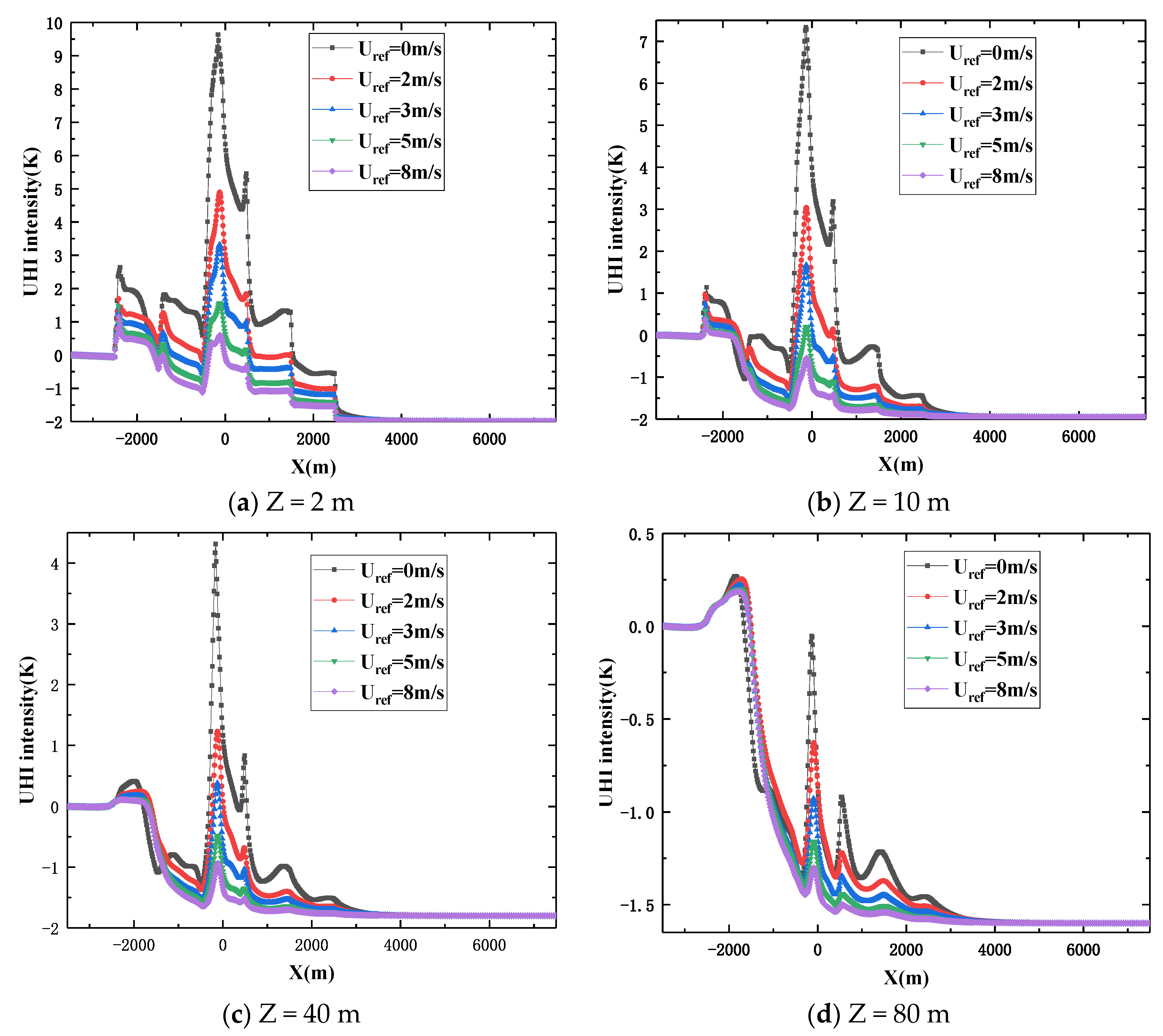
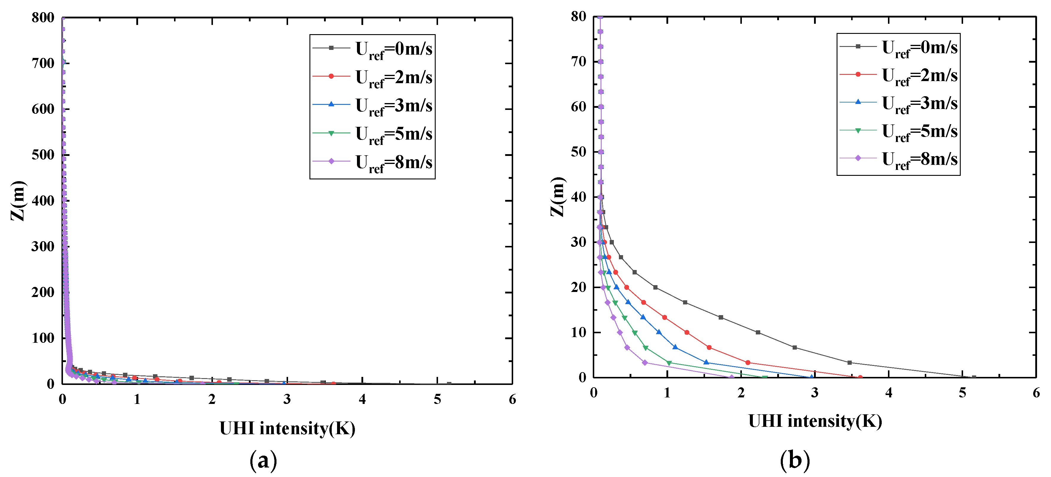
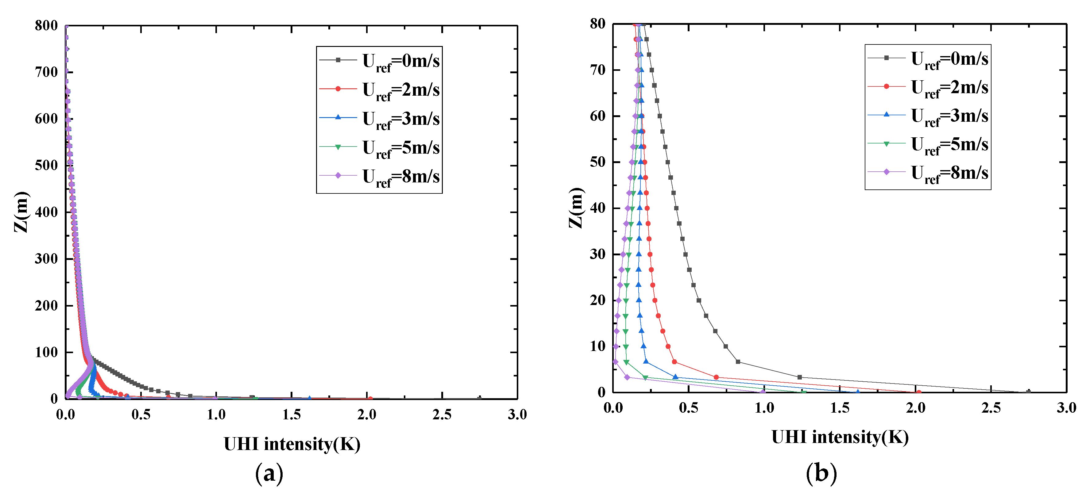
3.2.1. Influence of Ambient Crosswind Speed

The UHI effects are influenced by many factors. Memon et al. [43] summarized these factors and proposed some effective measures to reduce the UHI effect. Appropriate urban planning and design can induce wind into the city as so to alleviate the UHI phenomenon [44]. Some scholars used linear and nonlinear regression equations to predict the UHI intensity. They discovered that the UHI intensity decreased linearly with the wind speed [45,46]. In this study, we discussed the influence of wind speed on the UHI intensity in the urban area with a concentric structure, the porosity in the urban area from the inside to the outside was set to be 0.6 to 0.8, and the artificial heat intensity was 80 W/m², 60 W/m², and 40 W/m², respectively. The ambient crosswind speeds were set to be 0 m/s, 2 m/s, 3 m/s, 5 m/s, and 8 m/s, respectively, to explore the influence of wind on the UHI effect.

Figure 9 displays the profiles of UHI intensities at various heights with different ambient wind speeds. The lower the ambient speed, the higher the UHI intensity is. The UHI intensity is the highest when there is no wind in the city, especially in the central business district. A strong UHI effect is observed in the front of residential areas. A low-speed wind has a limited capacity to dissipate the artificial heat. The UHI effect is generated in front of the transition zone and the central business district.

As displayed in Figure 9, with wind speed increasing from 2 m/s to 3 m/s, UHI intensity decreases from the upstream boundary of the city to the downstream exit. At the height of 2 m (Figure 9a), increasing the wind speed by 1 m/s reduces the UHI intensity by about 1.9 K, which is consistent with the results informed by Memon and Leung [47]. The range and amplitude of the decrease in the UHI intensity are significantly reduced in the whole region with the wind speed increasing from 3 m/s to 5 m/s, with the greatest decrease of 1.7 K in the UHI intensity in the central urban area.

Regardless of wind speed, upstream transition area and residential area are hotter than the downstream transition area and residential area. The reason is that the maximum TKE is generated on the windward side of the central urban area. The turbulent shear stress transfers the energy and airflow downward on the leeward side of the central business district (vertical speed is negative), bringing the upper air into an urban porous medium area. Therefore, the low-temperature air at the top of the city moves downward on the leeward side of the city, reducing the UHI effect on the leeward side.

Figure 10 displays the vertical profiles of UHI intensities at various ambient crosswind speeds in the plane x = −2500 m. A strong UHI effect is observed in front of the residential areas of the city (x = −2500 m) since wind speed is smaller than that in the other city areas at the same altitude. The low-speed wind is not conducive to dissipate urban heat. The UHI intensity is significantly higher at the bottom than that on the top of the urban area. The UHI intensity at the height of the residential area is higher than that above the residential area, and the UHI intensity above the height of the residential area decreases rapidly with the height increasing. At heights exceeding 40 m, the UHI effect is not noticeable.

Figure 11 shows the vertical profiles of the UHI intensities at various ambient crosswind speeds in the center of the upstream residential area (x=−2000 m). With the height increasing, the UHI intensity gradually decreases. At heights greater than 20 m, the heat generated in front of the residential area is more likely to diffuse to the downstream area because the front residential area is not affected by the resistance of the urban porous medium area. Therefore, the UHI intensity in the center of the upstream transition zone is higher than that in the other areas. At the heights exceeding the urban canopy, the UHI intensity does not continue to increase but gradually decreases with the height increasing. There is no UHI effect at heights greater than 500 m.

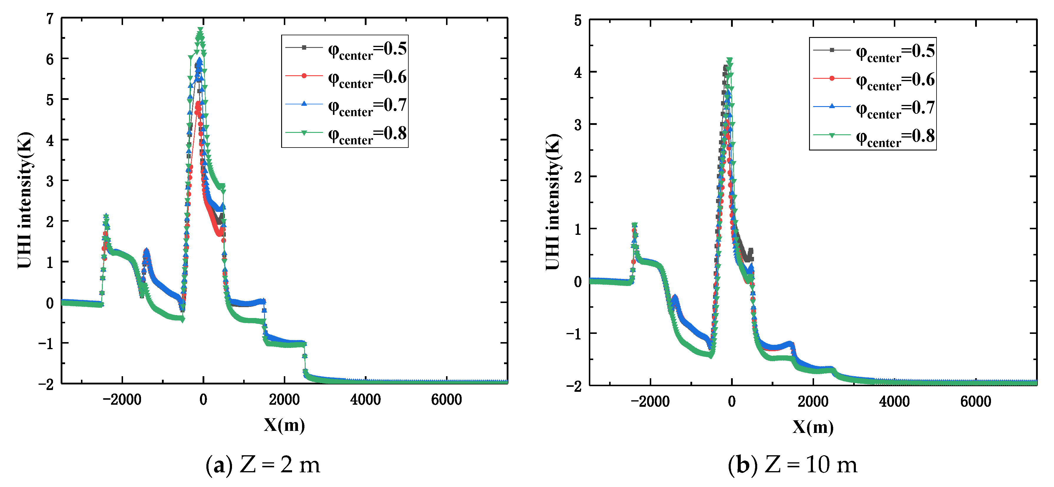
3.2.2. Influence of Porosity in the Central Urban Area

In a real urban area, the sum of building density and porosity is 1, and the range of building density is 0.18~0.62; thus, the range of the fluid porosity is 0.38~0.82 [48]. The intensity of artificial thermal sources in urban areas remains unchanged. Porosities of residential area and transition area are 0.8 and 0.7, respectively. We set the porosity of the central business district to be 0.5, 0.6, 0.7, and 0.8 to analyze the influence of the building density of the urban central business district on the UHI effect.

As shown in Figure 12, the smaller the porosity and the higher the building density, the greater the Darcy force and Forchheimer force will be, inhibiting more airflow. If the intensity of the artificial heat source in the central business district remains unchanged, the greater the porosity in the central business district, the smaller the Darcy force and Forchheimer force will be. Thus, the heat generated in the upstream transition zone can easily diffuse to the central business district. The temperature in the central area is dramatically higher than that in the other areas when porosity of the central business district is 0.8. Since the porosity of the downstream transition zone is lower than that of the central business district, the airflow is greatly inhibited, and the heat in the central business district cannot be diffuse downstream. When the porosity of the central business district is 0.5, large Darcy and Forchheimer forces will be generated. When the air flows from the upstream transition zone to downstream, it bypasses the central business district due to its large flow resistance. As a result, the heat in the central area cannot diffuse downstream, causing the increment of UHI intensity in the central business district. UHI effect is similar to the porosity of 0.5 and 0.7 in the central business district. Therefore, the porosity in the central business district has an optimal value at which the heat in the central business district can easily diffuse downstream. In the four cases analyzed in this paper, the optimal porosity value in the central urban area is 0.6.

At a height of 2 m from the ground (Figure 12a), the UHI intensity increases rapidly in the upper reaches of the city. At a height of 10 m (Figure 12b), the UHI effect in the upstream transition zone is not obvious. At a height of 40 m (Figure 12c), the maximum UHI intensity in the central business district is 1.7 K. At a height of 80 m (Figure 12d), UHI intensity of the central business district is significantly lower.

3.2.3. Influence of Anthropogenic Heat in the Central Business District

Studies on the intensity of anthropogenic heat sources in a large number of cities [49,50] have shown that anthropogenic heat intensifies the UHI effect [48,51,52]. Bhuian et al. [53] analyzed the land surface temperature (LST) data from 2000 to 2019 and concluded that population, lack of greenery and man-made heat are the main factors affecting the urban heat island effect. Yao et al. [54] conducted a combined analysis on satellite data and station data and concluded that human activities are the main driving force leading to the increase of the canopy layer UHI and surface UHI. We assume the intensity of the anthropogenic heat source Q in the central business district to be 40 W/m², 60 W/m², 80 W/m², 100 W/m² to investigate the influence of anthropogenic heat on the UHI effect. The porosities inside and outside of the urban area are 0.6 and 0.8, respectively. The intensities of the artificial heat source in the residential area and the transition area are 40 W/m² and 60 W/m².

As shown in Figure 13, as the intensity of the artificial heat source in the central urban area increases, the UHI intensity in the area increases significantly. The heat source intensity has no effect on the UHI intensity on the downstream transition area and residential area. The first strong UHI effect occurs in front of the city. As the airflow enters the urban area, part of it flows over the city due to the effect of the urban buildings, creating a high wind speed area above the windward edge of the city. The high-speed wind increases heat exchange flux, rapidly dissipating the city’s anthropogenic heat. Therefore, the UHI effect is the largest in front of the three urban porous medium areas, followed by a decline in the UHI intensity.

At a height of 2 m from the ground (Figure 13a), with anthropogenic heat source intensity increasing, the UHI intensity in the central urban area is also increasing, with a maximum value of 4.5 K. At a height of 10 m (Figure 13b), the heat diffuses to the central urban area due to the ambient crosswind, and no UHI effect is observed in the upstream transition area. At a height of 40 m (Figure 13c), there is no sudden increase in the UHI intensity at the front of the city. At a height of 80 m (Figure 13d), there is no UHI effect in the entire area because the height of the upstream buildings is lower than 40 m.

4. Discussion

In this paper, we used the modified turbulent porous method to calculate temperature and velocity distribution in a city with a concentric circular structure. The impact of three factors (i.e., artificial heat, incoming flow speed, and porosity in the central area) on the turbulent flow and heat transfer in the central urban area of a simplified city model with a concentric circular structure was analyzed. The simulation method allows the analysis of the UHI effect at the macroscale, provides high calculation accuracy and does not require high computing power.

Nevertheless, this study has several limitations, which will be addressed in our research in the next stage. First, we assumed that the city was a homogeneous porous medium. The porosity was constant in the calculation, and the anisotropy of the porous medium was not considered. In addition, the city model was relatively small and consisted of a simplified concentric circle structure that ignored the influence of urban blocks on the UHI effect. Second, the geometric city model was symmetrical, and neither the city morphology nor the effect of predominant wind direction on UHI effect was considered. Moreover, it was assumed that an ideal value of one-third of the solar radiation intensity was absorbed by the ground, in accordance with previous experimental and empirical research data. In reality, absorption of solar radiation by the ground is affected by cloud reflection and scattering, aerosol scattering and absorption, water vapor absorption, and other factors before reaching the earth’s surface.

Therefore, in the future study, we will consider the anisotropy of the porous structure and different porosities, depending on the multi-spatial characteristics of the urban structure in different directions. In addition, the effect of the city spatial form on the UHI effect will be considered in our future work. Optimizing the urban spatial form is one of the important measures to alleviate UHI. Guo et al. [55] considered the urban spatial morphology at the community scale and discussed the spatial differentiation characteristics and the driving factors of land surface temperature (LST) of the urban area of Dalian from 2003 to 2018. Oke [56] used a simple scale model to study the influence of urban geometric shapes on urban heat islands. The experimental results show that the geometric shape of the canyon in the city center is the main factor t producing the UHI at night.

5. Conclusions

Porous media models can be used to research the impact of buildings on the UHI effect in modern cities This model can preserve good modeling accuracy but requires much less computational resource. In this paper, a porous method was used to analyze spatial influence of ambient crosswind speed, porosity, and anthropogenic heat source intensity in the central business district on the UHI effect of a city with a concentric circle pattern. The important conclusions are drawn as follows:

• The extent of the UHI effect is significantly affected by the ambient crosswind speed. An increase in the wind speed significantly reduces the UHI intensity, especially in the central area of a city. A 1 m/s increase in the wind speed reduces the UHI intensity by approximately 1.7–1.9 K.
• In concentric circle cities, an optimal porosity exists for the city central area that facilitates artificial heat dissipation. In this study, the optimal porosity value was about 0.6, and the heat dissipation performance was approximately the same for the porosity of 0.5 and 0.7.
• With anthropogenic heat source intensity increasing, the UHI intensity in the central business district is also increasing, with a maximum value of 4.5 K at the measured height of 10 m. The rate of increase in the UHI intensity in the central business district is influenced by the upstream area.

References

1. Zhong, S.; Qian, Y.; Zhao, C.; Leung, R.; Yang, X.Q. A case study of urbanization impact on summer precipitation in the Greater Beijing Metropolitan Area: Urban heat island versus aerosol effects. J. Geophys. Res. Atmos. 2015, 120, 10,903–10,914. [Google Scholar] [CrossRef]
2. Grimmond, S.C.; Oke, T.R. Aerodynamic properties of urban areas derived from analysis of surface form. J. Appl. Meteorol. 1999, 38, 1262. [Google Scholar] [CrossRef]
3. Manley, G. On the Frequency of Snowfall in Metropolitan England. Q. J. R. Meteorol. Soc. 1958, 84, 70–72. [Google Scholar] [CrossRef]
4. Mathew, A.; Khandelwal, S.; Kaul, N. Spatial and temporal variations of urban heat island effect and the effect of percentage impervious surface area and elevation on land surface temperature: Study of Chandigarh city, India. Sustain. Cities Soc. 2016, 26, 264–277. [Google Scholar] [CrossRef]
5. Huang, L.; Li, J.; Zhao, D.; Zhu, J. A fieldwork study on the diurnal changes of urban microclimate in four types of ground cover and urban heat island of Nanjing, China. Build. Environ. 2008, 43, 7–17. [Google Scholar] [CrossRef]
6. Sun, C.Y.; Kato, S.; Gou, Z. Application of Low-Cost Sensors for Urban Heat Island Assessment: A Case Study in Taiwan. Sustainability 2019, 11, 2759. [Google Scholar] [CrossRef] [Green Version]
7. Sultana, S.; Satyanarayana, A. Urban heat island intensity during winter over metropolitan cities of India using remote-sensing techniques: Impact of urbanization. Int. J. Remote. Sens. 2018, 39, 6692–6730. [Google Scholar] [CrossRef]
8. Singh, P.; Kikon, N.; Verma, P. Impact of land use change and urbanization on urban heat island in Lucknow city, Central India. A remote sensing based estimate. Sustain. Cities Soc. 2017, 32, 100–114. [Google Scholar] [CrossRef]
9. Mirzaei, P.A.; Haghighat, F. Approaches to study Urban Heat Island–Abilities and limitations. Build. Environ. 2010, 45, 2192–2201. [Google Scholar] [CrossRef]
10. Khan, S.M.; Simpson, R.W. Effect Of A Heat Island On The Meteorology Of A Complex Urban Airshed. Bound. Layer Meteorol. 2001, 100, 487–506. [Google Scholar] [CrossRef]
11. Atkinson, B.W. Numerical Modelling of Urban Heat-Island Intensity. Bound. Layer Meteorol. 2003, 109, 285–310. [Google Scholar] [CrossRef]
12. Takahashi, K.; Yoshida, H.; Tanaka, Y.; Aotake, N.; Wang, F. Measurement of thermal environment in Kyoto city and its prediction by CFD simulation. Energy Build. 2004, 36, 771–779. [Google Scholar] [CrossRef]
13. Yushkov, V.P.; Kurbatova, M.M.; Varentsov, M.I.; Lezina, E.A.; Kallistratova, M.A. Modeling an Urban Heat Island during Extreme Frost in Moscow in January 2017. Izv. Atmos. Ocean. Phys. 2019, 55, 389–406. [Google Scholar] [CrossRef]
14. Vitanova, L.L.; Kusaka, H. Study on the Urban Heat Island in Sofia City: Numerical Simulations with Potential Natural Vegetation and Present Land Use Data. Sustain. Cities Soc. 2018, 40, 110–125. [Google Scholar] [CrossRef]
15. Jian, H.; Yuguo, L. Wind Conditions in Idealized Building Clusters: Macroscopic Simulations Using a Porous Turbulence Model. Bound. Layer Meteorol. 2010, 136, 129–159. [Google Scholar]
16. Parker, J.C.; Lenhard, R.J.; Kuppusamy, T. A parametric model for constitutive properties governing multiphase flow in porous media. Water Resources Res. 1987, 23, 618–624. [Google Scholar] [CrossRef]
17. Uth, M.F.; Jin, Y.; Kuznetsov, A.V.; Herwig, H. A direct numerical simulation study on the possibility of macroscopic turbulence in porous media: Effects of different solid matrix geometries, solid boundaries, and two porosity scales. Phys. Fluids 2016, 28, 70–77. [Google Scholar] [CrossRef]
18. Jin, Y.; Uth, M.F.; Kuznetsov, A.; Herwig, H. Numerical investigation of the possibility of macroscopic turbulence in porous media: A direct numerical simulation study. J. Fluid Mech. 2015, 766, 76–103. [Google Scholar] [CrossRef]
19. Nimvari, M.E.; Maerefat, M.; Jouybari, N.F.; El-Hossaini, M.K. Numerical simulation of turbulent reacting flow in porous media using two macroscopic turbulence models. Comput. Fluids 2013, 88, 232–240. [Google Scholar] [CrossRef]
20. Getachew, D.; Minkowycz, W.J.; Lage, J.L. A Modified Form of the k–ε Model for Turbulent Flows of an Incompressible Fluid in Porous Media. Int. J. Heat Mass Transf. 2000, 43, 2909–2915. [Google Scholar] [CrossRef]
21. Whitaker, S. The Forchheimer equation: A theoretical development. Transp. Porous Media 1996, 25, 27–61. [Google Scholar] [CrossRef]
22. Antohe, B.V.; Lage, J.L. A general two-equation macroscopic turbulence model for incompressible flow in porous media-ScienceDirect. Int. J. Heat Mass Transf. 1997, 40, 3013–3024. [Google Scholar] [CrossRef]
23. Brown, M.J. Comparison of Centerline Velocity Measurements Obtained around 2d and 3d Building Arrays in a Wind Tunnel. In Proceedings of the International Society of Environmental Hydraulics Conference, Tempe, AZ, USA, 5–8 December 2001. [Google Scholar]
24. Lien, F.S.; Yee, E.; Cheng, Y. Simulation of mean flow and turbulence over a 2D building array using high-resolution CFD and a distributed drag force approach. J. Wind. Eng. Ind. Aerodyn. 2004, 92, 117–158. [Google Scholar] [CrossRef]
25. Hu, Z.; Yu, B.; Chen, Z.; Li, T.; Min, L. Numerical investigation on the urban heat island in an entire city with an urban porous media model. Atmos. Environ. 2012, 47, 509–518. [Google Scholar] [CrossRef]
26. Jian, H.; Li, Y. Macroscopic simulations of turbulent flows through high-rise building arrays using a porous turbulence model. Build. Environ. 2012, 49, 41–54. [Google Scholar]
27. Wang, X.; Li, Y.; Hang, J. A combined fully-resolved and porous approach for building cluster wind flows. Build. Simul. 2017, 10, 97–109. [Google Scholar] [CrossRef]
28. Wang, X.; Li, Y. Predicting urban heat island circulation using CFD. Build. Environ. 2016, 99, 82–97. [Google Scholar] [CrossRef]
29. Chen, G.; Yang, X.; Yang, H.; Hang, J.; Lin, Y.; Wang, X.; Liu, Y. Integrated impacts of tree planting and street aspect ratios on CO dispersion and personal exposure in full-scale street canyons. Build. Environ. 2019, 169, 106529. [Google Scholar]
30. Fan, Y.; Hunt, J.; Li, Y. Buoyancy and turbulence-driven atmospheric circulation over urban areas. J. Environ. Sci. 2017, 59, 63–71. [Google Scholar] [CrossRef]
31. Chen, G.; Yang, X.; Yang, H.; Hang, J.; Lin, Y.; Wang, X.; Liu, Y. The influence of aspect ratios and solar heating on flow and ventilation in 2D street canyons by scaled outdoor experiments-ScienceDirect. Build. Environ. 2020, 185, 107159. [Google Scholar] [CrossRef]
32. Chen, G.; Wang, D.; Wang, Q.; Li, Y.; Wang, K. Scaled outdoor experimental studies of urban thermal environment in street canyon models with various aspect ratios and thermal storage. Sci. Total. Environ. 2020, 726, 138147. [Google Scholar] [CrossRef]
33. Gu, Z.L.; Zhang, Y.W. Large eddy simulation methods and application for building and urban wind environment simulation. Beijing Sci. Press. 2014, 64, 47–81. [Google Scholar]
34. Burgess, E.W. The Growth of the City: An Introduction to a Research Project; University of Chicago Press: Chicago, IL, USA, 2008. [Google Scholar]
35. Fernando, H.J.S. Fluid Dynamics of Urban Atmospheres in Complex Terrain. Annu. Rev. Fluid Mech. 2010, 42, 365–389. [Google Scholar] [CrossRef]
36. Ritter, B.R.E.; Hanna, S.R. Flow and dispersion in urban areas. Annu. Rev. Fluid Mech. 2003, 35, 469–496. [Google Scholar] [CrossRef]
37. Zuev, V.E.; Kas’Yanov, E.I.; Titov, G.A. Radiative characteristics of the system ‘broken cloudiness-underlying surface’. In Proceedings of the SPIE-The International Society for Optical Engineering, San Diego, CA, USA, 12–14 July 1993. [Google Scholar]
38. Martínez-Chico, M.; Batlles, F.J.; Bosch, J.L. Cloud classification in a mediterranean location using radiation data and sky images-ScienceDirect. Energy 2011, 36, 4055–4062. [Google Scholar] [CrossRef]
39. Zhang, N.; Wang, X.; Peng, Z. Large-Eddy Simulation of Mesoscale Circulations Forced by Inhomogeneous Urban Heat Island. Bound. Layer Meteorol. 2014, 151, 179–194. [Google Scholar] [CrossRef]
40. Rajapaksha, I.; Nagai, H.; Okumiya, M. A ventilated courtyard as a passive cooling strategy in the warm humid tropics. Renew. Energy 2003, 28, 1755–1778. [Google Scholar] [CrossRef]
41. Leung, K.K.; Liu, C.H.; Wong, C.; Lo, J.; Ng, G. On the study of ventilation and pollutant removal over idealized two-dimensional urban street canyons. Build. Simul. 2012, 5, 359–369. [Google Scholar] [CrossRef]
42. Wang, H.; Peng, C.; Li, W.; Ding, C.; Zhou, N. Porous media: A faster numerical simulation method applicable to real urban communities. Urban Climate. 2021, 38, 100865. [Google Scholar] [CrossRef]
43. Memon, R.A.; Leung, D.; Liu, C. A review on the generation, determination and mitigation of Urban Heat Island. J. Environ. Sci. 2008, 20, 120–128. [Google Scholar]
44. He, B.J.; Ding, L.; Prasad, D.K. Urban ventilation and its potential for local warming mitigation: A field experiment in an open low-rise gridiron precinct. Sustain. Cities Soc. 2020, 55, 102028. [Google Scholar] [CrossRef]
45. Morris, C.; Simmonds, I.; Plummer, N. Quantification of the Influences of Wind and Cloud on the Nocturnal Urban Heat Island of a Large City. J. Appl. Meteorol. 1992, 40, 169–182. [Google Scholar] [CrossRef]
46. Schlünzen, K.; Hoffmann, P.; Rosenhagen, G.; Riecke, W. Long-term changes and regional differences in temperature and precipitation in the metropolitan area of Hamburg. Int. J. Climatol. 2010, 30, 1121–1136. [Google Scholar] [CrossRef]
47. Memon, R.A.; Leung, D. Impacts of environmental factors on urban heating. J. Environ. Sci. 2010, 12, 1903–1909. [Google Scholar] [CrossRef]
48. Kikegawa, Y.; Genchi, Y.; Yoshikado, H.; Kondo, H. Development of a numerical simulation system toward comprehensive assessments of urban warming countermeasures including their impacts upon the urban buildings’ energy-demands. Appl. Energy 2003, 76, 449–466. [Google Scholar] [CrossRef]
49. Kato, S.; Yamaguchi, Y. Analysis of urban heat-island effect using ASTER and ETM+ Data: Separation of anthropogenic heat discharge and natural heat radiation from sensible heat flux. Remote. Sens. Environ. 2005, 99, 44–54. [Google Scholar] [CrossRef]
50. Offerle, B.; Grimmond, C.; Fortuniak, K. Heat storage and anthropogenic heat flux in relation to the energy balance of a central European city centre. Int. J. Climatol. 2005, 25, 1405–1419. [Google Scholar] [CrossRef]
51. Ichinose, T.; Shimodozono, K.; Hanaki, K. Impact of anthropogenic heat on urban climate in Tokyo. Atmos. Environ. 1999, 33, 3897–3909. [Google Scholar] [CrossRef]
52. Du, H.; Wang, D.; Wang, Y.; Zhao, X.; Fei, Q.; Hong, J.; Cai, Y. Influences of land cover types, meteorological conditions, anthropogenic heat and urban area on surface urban heat island in the Yangtze River Delta Urban Agglomeration. Sci. Total. Environ. 2016, 571, 461–470. [Google Scholar] [CrossRef] [PubMed]
53. Bhuian, M.H.; Dewan, A.; Mahmud, G.I.; Hassan, Q.K.; Kiselev, G. Surface urban heat island intensity in five major cities of Bangladesh: Patterns, drivers and trends. Sustain. Cities Soc. 2021, 71, 102926. [Google Scholar]
54. Yao, R.; Wang, L.; Huang, X.; Liu, Y.; Wang, L. Long-term trends of surface and canopy layer urban heat island intensity in 272 cities in the mainland of China. Sci. Total. Environ. 2021, 772, 145607. [Google Scholar] [CrossRef] [PubMed]
55. Guo, A.D.; Yang, J.; Xiao, X.M.; Xia, J.H.; Jin, C.; Li, X.M. Influences of urban spatial form on urban heat island effects at the community level in China. Sustain. Cities Soc. 2019, 53, 101972. [Google Scholar] [CrossRef]
56. Oke, T.R. Canyon geometry and the nocturnal urban heat island: Comparison of scale model and field observations. Int. J. Climatol. 2010, 1, 237–254. [Google Scholar] [CrossRef]
Figure 1. The evolution of the geometric model: (a) Map of London; (b) three-dimensional geometric model and boundary conditions.
Energies 14 04681 g001
Figure 2. Schematic diagram of the grid demarcation.
Energies 14 04681 g002
Figure 3. Grid independence test results.
Energies 14 04681 g003
Figure 4. Field measurement sites and photo of measuring instruments.
Energies 14 04681 g004
Figure 5. The location of the measurement points.
Energies 14 04681 g005
Figure 6. The contours of wind velocity in plane z = 2 m: (a) macroscale porous media model simulation, (b) microscale simulation (for southerly wind).
Energies 14 04681 g006
Figure 7. (a) Comparison of measurement data with the standard simulation results (b) Comparison of the measurement data with standard simulation, and porous simulation results.
Energies 14 04681 g007
Figure 8. Distribution of (a) horizontal velocity, (b) vertical velocity, (c) TKE, (d) TEK microscale simulation results (building zone), (e) TEK macroscale simulation results (porous medium zone) in plane y = 0 when the wind speed is 2 m/s.
Energies 14 04681 g008aEnergies 14 04681 g008b
Figure 9. The horizontal profiles of the UHI intensities at different ambient crosswind speeds at heights of (a) 2 m, (b) 10 m, (c) 40 m, and (d) 80 m in the plane y = 0.
Energies 14 04681 g009
Figure 10. The vertical profiles of the UHI intensities at different ambient crosswinds in the plane x = −2500 m: (a) within the computational height and (b) at the urban canopy’s heights.
Energies 14 04681 g010
Figure 11. The vertical profiles of the UHI intensities at different ambient crosswinds in the plane x = −2000 m: (a) within the computational height and (b) at the urban canopy’s heights.
Energies 14 04681 g011
Figure 12. The horizontal profiles of the UHI intensities at different porosities in the central business district at the height of (a) 2 m, (b) 10 m, (c) 40 m, and (d) 80 m in the plane y = 0.
Energies 14 04681 g012aEnergies 14 04681 g012b
Figure 13. The horizontal profiles of the UHI intensities at different intensities of the artificial heat source at the heights of (a) 2 m, (b) 10 m, (c) 40 m, and (d) 80 m in plane y = 0.
Energies 14 04681 g013