The Potential of Vehicle-to-Grid to Support the Energy Transition: A Case Study on Switzerland

Abstract

Energy systems are undergoing a profound transition worldwide, substituting nuclear and thermal power with intermittent renewable energy sources (RES), creating discrepancies between the production and consumption of electricity and increasing their dependence on greenhouse gas (GHG) intensive imports from neighboring energy systems. In this study, we analyze the concurrent electrification of the mobility sector and investigate the impact of electric vehicles (EVs) on energy systems with a large share of renewable energy sources. In particular, we build an optimization framework to assess how Evs could compete and interplay with other energy storage technologies to minimize GHG-intensive electricity imports, leveraging the installed Swiss reservoir and pumped hydropower plants (PHS) as examples. Controlling bidirectional EVs or reservoirs shows potential to decrease imported emissions by 33–40%, and $60\%$ can be reached if they are controlled simultaneously and with the support of PHS facilities when solar PV panels produce a large share of electricity. However, even if vehicle-to-grid (V2G) can support the energy transition, we find that its benefits will reach their full potential well before EVs penetrate the mobility sector to a large extent and that EVs only contribute marginally to long-term energy storage. Hence, even with a widespread adoption of EVs, we cannot expect V2G to single-handedly solve the growing mismatch problem between the production and consumption of electricity.

1. Introduction

Worldwide, energy sectors are facing profound changes following the Paris Agreement pledges to limit global warming to well below 2 °C [1]. This will require significant investments in renewable energy sources (RES) to meet the electricity demand while complying with the wanted reduction of greenhouse gas (GHG) emissions. Generally, solar and wind-based energy generation is envisioned to cover the largest part of the increasing gap between the production and consumption of electricity following the decommissioning of baseload nuclear and thermal power plants [2].

1.1. The Mismatch between Electricity Production and Consumption

Replacing the current baseload with RES will however emphasize already existing diurnal and seasonal discrepancies: while photovoltaic (PV) panels mainly produce electricity at noon and in summer, the energy demand is on the other hand high in the evenings and in winter when heating is required, especially in temperate or continental climates. Future power systems will thus face an important mismatch problem, where electricity consumption and production are not aligned [3,4]. When no storage capacity is available, this will indeed force such power systems to export surpluses of energy to connected energy markets during summer or when the sun is shining. Conversely, to cover the domestic demand in the evenings and over the winter period, electricity will have to be imported once the stored energy is depleted. However, imported electricity may have a high GHG content compared to the domestic production of energy systems with a large share of renewable sources when it comes from emission-intensive coal or gas power plants [5].

Alternatively to exchanges with connected power systems, the increasing sharp afternoon ramp-up and evening peak net demand could be covered by additional power plants. However, this would require significant investments in fast-ramping energy resources and in so-called peaking units—power plants that only operate for short periods of time to meet the evening peak demand. Moreover, the plants chosen for these tasks are usually fast thermal power plants when hydropower plants are not available, which would jeopardize the global efforts to decrease our carbon footprint [6,7].

On the other hand, control strategies can provide alternative solutions to mitigate this issue by leveraging a collection of storage technologies to support electricity grids and dampen diurnal and seasonal discrepancies between the production and consumption of electricity. Dujardin et al. [8] for example showed that the already installed hydropower plants could be used to help mitigate the growing reliance of a fully renewable Switzerland on the European grid to some extent. Following the global electrification of mobility, additional storage possibilities will arise due to the increasing number of electric vehicles (EVs) connected to power grids.

1.2. The Role of Electric Vehicles

More than 10 million EVs were on the road around the world in 2020, and this number is growing exponentially each year [9]. From an energy system’s perspective, EVs are batteries moving from one point of the electricity grid to another, with potentially negative impacts if many of them are connected to the grid and charging simultaneously.

Several studies in the literature analyzed the effects of controlled charging and discharging of EVs on the grid and the associated reductions of GHG emissions [10,11,12,13,14,15,16]. Note that, in energy systems with a large share of RES, flattening the duck curve, which represents the net demand of a power system once the intermittent renewable energy production has been subtracted from the total demand [3], is similar to reducing the amount of imported GHG emissions. Indeed, a more pronounced duck curve inevitably leads to more imports from neighboring countries, which, in such systems, means an increase in the GHG intensity of the electricity.

In general, controlling EVs was shown to flatten the duck curve to some extent, both when considering controlled charging (V1G) [10] or vehicle-to-grid (V2G) operations [11,12,13,14]. At the city level, significant reductions of carbon emissions can be attained in systems with large solar power generation and EV penetration, e.g., as shown in a case study in Kyoto [15]. Similarly, in Utrecht, Brinkel et al. [16] found that V2G could reduce emissions of up to $23.6$%. Finally, a large-scale study on the electricity grid in the midwestern United States showed that V2G could almost completely level the daily variations of the duck curve [12]. However, none of these works considers how EVs could collaborate with other storage technologies to support the grid.

1.3. Main Contributions

In this work, we investigate how energy storage technologies can minimize the amount of GHG-intensive electricity imports needed to cover the domestic demand with a case study on Switzerland. We first analyze the potential of controlling EVs, with V1G or V2G, to reduce these emissions. We then assess how V1G and V2G could compete or collaborate with other energy storage technologies in different energy and mobility scenarios and under shorter or longer optimization horizons, using the existing reservoir and pumped hydropower plants in Switzerland as examples. We simultaneously analyze the influence of these different control strategies on the dependency of energy systems with a large share of RES on connected systems for energy exchanges. Finally, we briefly investigate the impacts of V1G and V2G on the degradation of EV batteries to discuss the downside of these control strategies.

1.4. Structure of the Work

The rest of the work is structured as follows. Section 2 introduces the needed background knowledge and Section 3 then details the methods used in this work. Finally, we present and discuss the results in Section 4 and subsequently conclude the paper in Section 5.

2. Background

This Section provides necessary information on the Swiss energy system, as well as a small overview of the different EV charging strategies.

2.1. Challenges of the Future Swiss Energy System

The global energy transition is emphasized further in Switzerland due to the planned nuclear phase-out [17]. This baseload, which currently represents one-third of the total electricity production in the country, will have to be replaced before 2035 when the nuclear power plants are scheduled for decommissioning [18]. On the other hand, the heating and mobility sectors, currently responsible for almost one-half of the total domestic GHG emissions [19], will also undergo deep transitions leading to an increase in electricity demand. Additionally, almost 50,000 EVs were registered in Switzerland as of 2020, and this number is growing steadily every year [20], with projections for 2050 ranging between $1.4$ and $3.5$ million EVs [21,22], which will further augment the electricity consumption in the country.

Switzerland currently mostly relies on nuclear and hydro-based power plants, with numerous reservoirs and run-of-the-river (RoR) installations, to produce the large majority of its electricity [23]. The remaining 8–9% is generated via renewable energy sources, for the bigger part, and some conventional thermal power plants. Since more than 50% of its electricity generation is supported by hydrological sources, Switzerland is however heavily dependent on its water cycle: the snowmelt in spring and throughout summer generates hydropower surpluses that are currently exported to neighboring countries, while the dams are on the other hand depleted during the winter, forcing the country to rely on imports to cover the increasing domestic heating demand. All year round, Switzerland is therefore steadily relying on energy exchanges with neighboring countries to compensate for the system-wide discrepancies between electricity production and consumption, taking advantage of its geographical position and comparatively small size in the middle of the European continent, as can be observed in Figure 1. This plot also exhibits how storage technologies—PHS facilities in that case—are utilized as of today, with more activity over the summer period when energy surpluses can be exploited.

Altogether, the Swiss electricity generation thus currently features a low GHG intensity profile [4]. Due to the higher GHG content of the imported electricity, there is a need for Switzerland to decrease its dependency on international exchanges to meaningfully follow its pledges to reduce carbon emissions [24]. Additionally, a large market penetration of solar panels was shown to be problematic for the country because of the limited cross-border net transfer capacities (NTC) [8]. Similarly, other analyses pointed out that the currently envisioned Swiss strategy to transfer almost all the nuclear electricity production to intermittent renewable sources would create bottlenecks on the cross-border lines [25,26].

2.2. EV Charging Strategies

In the Uncontrolled Charging (UC) regime, the classical charging protocol, people plug their vehicle directly upon arrival and it immediately starts to charge at full power until the maximum energy capacity is reached, thereby emphasizing the magnitude of the evening peak demand further [12,27].

However, control algorithms can mitigate the issues of UC and even leverage EV batteries to support the grid. Firstly, controlled charging (V1G) can regulate the power drawn from the grid to shift the charging of EVs to more suitable times and reduce grid stress. Moreover, if bidirectional EVs able to feed electricity back to the grid are available, they can participate in so-called vehicle-to-grid (V2G) operations. In that case, EVs are additionally able to shift the electricity production, and it was already observed that V2G could have an impact on the grid comparable to stationary battery storage systems [3,28]. Controlling the charging and discharging of EVs is, however, a much more challenging task than operating a stationary battery, due to their dynamical framework. EVs are indeed not always connected to the grid and their owners require to have enough energy for their coming trips any time they disconnect their vehicles, which brings both stochasticity and hard constraints in the control problem. Moreover, the impact of battery degradation on the benefits of V2G is still debated in the literature, where some studies argue that V2G is not economically viable for the participating EVs [29], or at least not for all of them [13].

3. Methods

In this study, we develop an optimization model to minimize the GHG emissions stemming from electricity imports in Switzerland. According to scenarios with different electricity production and consumption patterns and market penetration of EVs, we simulate the years 2018 (reference), 2030, 2035, and 2050 with a resolution of 15 min to assess the future evolution of the system. Based on a given fluctuating profile of the GHG content of the European grid, we investigate the potential reductions of imported GHG emissions that can be attained over each whole year through control algorithms. Note that we do not consider market forces and focus on reductions of GHG-intensive electricity imports, whereas financial incentives usually guide the operations of all the participants in reality. Nonetheless, assuming a very high cost of CO${}_2$ in the coming years, which could completely drive the price of electricity, similar behaviors to what is shown in this study could be expected.

Throughout this work, we either control the operations of EVs (V1G or V2G), reservoirs, Pumped Hydro Storage (PHS) facilities, or a combination thereof to minimize GHG-intensive imports. When not controlled, hydro-based solutions follow a historical activity pattern, while EVs employ UC mechanisms. To analyze the impact of perfect yearly forecasts of the production and consumption of electricity, the GHG-content of imports, and the behaviors of EVs, we compare the performance over one year to the cumulative performance over each week of the year. In this scheme, the optimization has perfect knowledge of all the variables over a restricted weekly horizon and can thus only find locally optimal solutions.

In this Section, we first provide information about the data inputs to our model in Section 3.1, detailing the creation of electricity production and consumption profiles and the modeling of electric vehicles. In Section 3.2, we then present the extrapolation scenarios used to project the data in future years. Finally, the optimization framework is laid out and explained in Section 3.3.

3.1. Data

3.1.1. Uncontrolled Supply and Demand Profiles

We compute profiles at a resolution of 15 min for each electricity producer and the electricity consumption from 2018, which is used as base year throughout this study, in Switzerland. These profiles are then scaled each year in the optimization horizon according to the total production or demand scenario, as presented in Section 3.2.

We use hourly profiles provided by Rüdisüli et al. [30] for the RoR, reservoir, PHS, nuclear, and PV electricity production. The reader is referred to the original paper for a description of the data processing. The hourly wind power output profile is retrieved from www.renewables.ninja (4 August 2021) where the data has been collected and preprocessed as explained in Staffell et al. [31] (see Appendix A for more details), and all these profiles are linearly interpolated to get consistent 15 minute profiles. Since the combined annual production of all the conventional thermal power plants is roughly constant in Switzerland [30], it is modeled as a fixed profile. Similarly, production profiles from energy sources not described above, e.g., from other renewable sources, are assumed constant throughout the study. The total constant production in the base year is derived from the annual Swiss electricity production data [32]. Finally, the electricity consumption profile used in this work originates from the Swiss Transmission System Operator (TSO) [33] and is adapted for each year in the horizon to account for the electrification of the heating sector as explained in Section 3.2.

When the electricity production of reservoirs is optimized by the controller, we cannot use the profile described above and have to rely on water inflows to know how much energy is available to the controlled power plants at each point in time. These inflows were provided by Beer et al. [34] for the base year 2018. Throughout the years of the optimization horizon, those inflows were scaled proportionally to the projected increase in reservoir capacity, see

Table A1. Summary of projected energy and power capacities of hydro-based powerplants in Switzerland.

Year	Energy Capacity	Power Capacity	Ramping Capacity
Reservoir
2018	8800 GW h	8.2 GW	755.6 MW/15 min
2030	9835 GW h	9.2 GW	844.4 MW/15 min
2035	10,353 GW h	9.7 GW	888.8 MW/15 min
2050	11,503 GW h	10.8 GW	987.6 MW/15 min
PHS
2018	300 GW h	3.1 GW	2400 MW/15 min
2030	335 GW h	3.5 GW	2400 MW/15 min
2035	353 GW h	3.7 GW	2400 MW/15 min
2050	392 GW h	4.1 GW	2400 MW/15 min

in Appendix B.

Finally, the hourly GHG content of the imported electricity from the European grid is taken from Rüdisüli et al. [22] and interpolated to get the desired resolution. Since the given profile presents daily patterns which only vary between seasons, we additionally incorporate Gaussian noise at each time step to model fluctuations from one day to another that can be exploited by our minimization framework. Note that we assume the GHG content of the European grid to follow the same trends over all scenarios, which does not take the current global energy transition into account. For further work, it would be more justified to characterize the GHG intensity of the imported electricity in terms of marginal rather than average emissions, as we do here, since any additional import in Switzerland would come from the marginal electricity producer of the foreign grid [35].

3.1.2. Electric Vehicles

To investigate the effects of UC, V1G, and V2G, we need to know how many EVs are connected to the grid at each point in time, how much energy they require for their next trip, and at which rate they can exchange power with the grid.

To define the activity pattern of each EV, we use 100 randomly sampled travel schedules from Pareschi et al. [36], who adapted the Swiss household travel survey (HTS) [37] to electric vehicles. A travel schedule describes the list of trips made by an EV, with the corresponding starting and ending locations, as well as the associated energy consumption, for one week in each season and at the resolution of one minute. Subsampling the travel schedules to 15 min intervals then gives the location of each EV at each point in time and their corresponding energy needs.

When parked, EVs can be located in four different categories of places: at home, at work, at a Point of Interest (POI), or at Other locations (POIs include education, entertainment or shopping activities, whereas Other represents locations far away from the purpose of the trip). Each category is assigned a certain probability to host a charging station with a given power rating capacity, as depicted in

Table 1. Charging station characteristics adopted in this work.

Location	Probability of a Station	Power Rating
Home	80% [38]	{$3.7$, $7.4$, 11} kW
Work	50% [39]	{11, 22} kW
Point of Interest	26% [37,39]	Distribution from [40]
Other	26% [37,39]	Distribution from [40]

. Together with the traveling schedule, we thus know how much power each EV can draw from or feed to the grid when parked.

Finally, each EV is assigned a type, which specifies its maximum energy and power capacity, to know how much power and energy can actually be exchanged with the grid. Based on values from the current market leaders in

Table A2. EV types used in this work, with their power and energy capacities, as well as their corresponding market share.

Model	Share	Energy	Power
Tesla Model S	$21.93$%	100 $\mathrm{k}$$\mathrm{W}$$\mathrm{h}$	250 $\mathrm{k}$$\mathrm{W}$
Renault Zoe	$18.37$%	41 $\mathrm{k}$$\mathrm{W}$$\mathrm{h}$	50 $\mathrm{k}$$\mathrm{W}$
Tesla Model 3	$18.27$%	75 $\mathrm{k}$$\mathrm{W}$$\mathrm{h}$	250 $\mathrm{k}$$\mathrm{W}$
BMW i3	$18.12$%	$42.2$ $\mathrm{k}$$\mathrm{W}$$\mathrm{h}$	50 $\mathrm{k}$$\mathrm{W}$
Tesla Model X	$8.89$%	100 $\mathrm{k}$$\mathrm{W}$$\mathrm{h}$	150 $\mathrm{k}$$\mathrm{W}$
Nissan Leaf	$6.11$%	62 $\mathrm{k}$$\mathrm{W}$$\mathrm{h}$	100 $\mathrm{k}$$\mathrm{W}$
Audi e-tron	$2.48$%	95 $\mathrm{k}$$\mathrm{W}$$\mathrm{h}$	150 $\mathrm{k}$$\mathrm{W}$
Mitsubishi i-MiEV	$1.95$%	16 $\mathrm{k}$$\mathrm{W}$$\mathrm{h}$	50 $\mathrm{k}$$\mathrm{W}$
Jaguar I-Pace	$1.84$%	90 $\mathrm{k}$$\mathrm{W}$$\mathrm{h}$	100 $\mathrm{k}$$\mathrm{W}$
Citroën C-ZERO	$0.82$%	$14.5$ $\mathrm{k}$$\mathrm{W}$$\mathrm{h}$	40 $\mathrm{k}$$\mathrm{W}$
Peugeot iOn	$0.66$%	16 $\mathrm{k}$$\mathrm{W}$$\mathrm{h}$	40 $\mathrm{k}$$\mathrm{W}$
Mercedes-Benz EQC	$0.55$%	100 $\mathrm{k}$$\mathrm{W}$$\mathrm{h}$	110 $\mathrm{k}$$\mathrm{W}$

, Appendix C, we randomly sample 100 times according to the given market shares to define the characteristics of each vehicle at the beginning of the optimization.

Altogether, this procedure defines how much energy and power is available for or required by the 100 EVs at each point in time. Their energy needs, energy capacities, and power ratings are then scaled to meet the total values for each scenario presented in Section 3.2.

3.2. Scenarios

To assess the evolution of the energy system from 2018 to 2030, 2035, and 2050, we scale the electricity profiles from Section 3.1.1 and the energy and power capacities of EVs from Section 3.1.2 to match the expected total electricity production and consumption in each year according to different scenarios.

We consider two energy scenarios to project the inland production and consumption of electricity, referred to as the business-as-usual (BAU) and ZERO scenarios. These closely follow scenarios from the Swiss Federal Office of Energy [2]. As can be observed in Figure 2, the ZERO scenario assumes a large installation of solar panels to recover from the loss of nuclear power. This is the main difference with the BAU scenario, where conventional thermal production fills most of the gap. Additionally, the BAU scenario assumes a higher annual demand for electricity of up to 77 TW h in 2050, 5.6 TW h more than in the ZERO scenario due to more ambitious energy efficiency and consumption reduction targets. Overall, it also entails a much lower total production of 72 TW h, since less solar electricity production is envisioned.

In all scenarios, the consumption profile is slightly modified to account for the expected electrification of the heating sector in Switzerland. First, the demand profile from heat pumps (HPs) in 2018, generated in Rüdisüli et al. [4], is subtracted from the base year consumption profile and scaled each year in the horizon depending on the annual heat pump electricity demand projection from the Swiss Office of Energy [2]. The remaining consumption profile is separately scaled to match the demand from either the BAU or ZERO scenario (after subtracting the expected HP demand). We finally add both profiles together to get a more accurate representation of the electricity demand in Switzerland throughout the years.

On the other hand, we also investigate the effect of the number of EVs connected to the grid on the optimization with two scenarios, the new-energy-policy (NEP) scenario, taken from the Energy Perspectives from 2012 [21], and the electric-based-mobility (EBM) scenario from Rüdisüli et al. [22]. In the former, a more conservative approach is adopted, assuming that $23\%$ of the entire stock of $6.1$ millions vehicles will be electric in 2050, while the latter projects a share of $58\%$. These values correspond to an additional electricity consumption of 3 $\mathrm{T}$$\mathrm{W}$$\mathrm{h}$ and $7.5$ $\mathrm{T}$$\mathrm{W}$$\mathrm{h}$, respectively, and the impact can be seen in Figure 2.

3.3. Optimization Framework

The power system controller can either control the power of charge or discharge of the EVs, the reservoirs, the PHS, or a combination thereof. All the EVs are aggregated in a virtual EV battery, as detailed in Section 3.3.1, and we will thus refer to the EV as being singular. Similarly, all the reservoirs and PHS are aggregated in two virtual variables by summing their power and energy values. When not optimized, reservoirs and PHS follow the historical profiles described in Section 3.1.1, scaled according to their total energy production in the corresponding year from Table A1 in Appendix B, and the charging of EVs is unmanaged.

Throughout this work, we define negative power flows as production of electricity in Switzerland and positive ones as consumption. To alleviate the computational burden that would arise from more complex models, we represent the power system via a linear program (LP). This requires separating charging and discharging power variables to keep the problem linear due to energy conversion inefficiencies. Altogether, the minimization of imported GHG emissions in Switzerland is formulated as follows, for a horizon of N time steps, corresponding to a week or a year (Since each time step represents 15 min, $N=4\times 24\times 7=672$ for a week and $N=4\times 24\times 365=\mathrm{35,040}$ for a full year):

$$\begin{array}{ccccc}\hfill & \underset{U_1,\dots ,U_N}{min}\hfill & \hfill & \sum _{t=1}^{t=N}{P}_t^{Imp}GH{G}_t^{EU}-\alpha P_t^{Exp}+\beta {ϵ}_t^{Imp}\hfill & \hfill \end{array}$$

(1a)

$$\begin{array}{ccc}\hfill & \mathrm{subject}\mathrm{to}\hfill & P_t^{Net}-P_t^{Imp}+P_t^{Exp}-P_t^{Res}+P_t^{PHS,c}-P_t^{PHS,d}+P_t^{EV,c}-P_t^{EV,d}=0\hfill \end{array}$$

(1b)

$$\begin{array}{cccc}\hfill & \hfill & & E_{t-1}^{EV}+{\eta }_{EV}{P}_t^{EV,c}-\frac{P_t^{EV,d}}{{\eta }_{EV}}-E_t^{EV,cons}+\Delta E_t^{EV,trips}=E_t^{EV}\hfill \end{array}$$

(1c)

$$\begin{array}{cccc}\hfill & \hfill & & E_{t-1}^{PHS}+{\eta }_{PHS}{P}_t^{PHS,c}-\frac{P_t^{PHS,d}}{{\eta }_{PHS}}=E_t^{PHS}\hfill \end{array}$$

(1d)

$$\begin{array}{cccc}\hfill & \hfill & & E_{t-1}^{Res}-\frac{P_t^{Res,d}}{{\eta }_{Res}}+{\mathrm{I}}_t=E_t^{Res}\hfill \end{array}$$

(1e)

$$\begin{array}{cccc}\hfill & \hfill & & 0\le P_t^{X,\{c,d\}}\le P_{t,max}^{X,\{c,d\}}\hfill \end{array}$$

(1f)

$$\begin{array}{cccc}\hfill & \hfill & & E_{t,min}^X\le E_t^X\le E_{t,max}^X\hfill \end{array}$$

(1g)

$$\begin{array}{cccc}\hfill & \hfill & & P_t^{X,\{c,d\}}-P_{t-1}^{X\{c,d\}}\le P_{max,ramp}^{X,\{c,d\}}\hfill \end{array}$$

(1h)

$$\begin{array}{cccc}\hfill & \hfill & & P_t^{EV,\{c,d\}}-P_{t-4}^{EV,\{c,d\}}\le 3*P_{max,ramp}^{EV,\{c,d\}}\hfill \end{array}$$

(1i)

$$\begin{array}{cccc}\hfill & \hfill & & 0\le P_t^{Imp}\le P_{max}^{Imp}+{ϵ}_t^{Imp}\hfill \end{array}$$

(1j)

$$\begin{array}{cccc}\hfill & \hfill & & 0\le P_t^{Exp}\le P_{max}^{Exp}\hfill \end{array}$$

(1k)

$$\begin{array}{cccc}\hfill & \hfill & & 0\le {ϵ}_t^{Imp}\hfill \end{array}$$

(1l)

where all the constraints (1b)–(1l) have to be satisfied at all time steps, indicated by the subscript $t=1,\dots ,N$. X represents constraints for each of the three controllable participants, i.e. reservoirs, PHS, and EVs. P stands for power and E for energy components, while the superscripts refer to which actor they correspond to: Imports (Imp), Exports (Exp), reservoirs (Res), PHS, or EV. $I_t$ is the water inflow and $P_t^{Net}$ the electricity consumption in Switzerland after the subtraction of the static production which cannot be controlled in this study, mainly from nuclear, RoR, and renewable energy sources. Additionally, the superscripts c and d stand for charging and discharging, respectively. The variables controlled in the optimization are grouped in U, i.e.:

$$\begin{array}{cc}\hfill U_t& \subseteq \{P_t^{Res},P_t^{PHS,c},P_t^{PHS,d},P_t^{EV,c},P_t^{EV,d}\}.\hfill \end{array}$$

(2)

$\eta$ represents conversion efficiencies, $\alpha \ge 0$ is a small constant and $\beta =1000$. Note that $P_{t,max}^{Res,c}=P_{max,ramp}^{Res,c}=0$ in Equations (1f) and (1h), as reservoirs cannot charge any energy.

The primary objective of the optimization is to minimize the sum of imported GHG from the European grid, represented by the first term of Equation (1a). However, we also slightly reward the model for exports in the second term to avoid simultaneous charging and discharging operations that would lead to energy losses due to conversion efficiencies. Indeed, this makes sure that the optimization is exporting electricity surpluses to neighboring countries, so that the observed power flows are representative of the state of the system. We choose $\alpha \ll GH{G}_{min}^{EU}$, the minimum GHG intensity of the European electricity, to ensure that rewards for exports can never be higher than penalties from imports. Otherwise, the model might import more energy than needed to export it later and get unwanted bonuses. This also guarantees that storing domestic energy surpluses is always preferred over exporting them. The last term in the objective is a penalty on slack variables, to make sure the model respects the constraints and does not use the slack variables when not needed.

Equation (1b) forces the production and consumption to match, including cross-border exchanges, while Equations (1c)–(1e) enforce conservation of energy throughout the process for the three variables we can control. For reservoirs, this includes energy stemming from water inflows throughout the horizon. The conversion efficiencies are set to ${\eta }_{PHS}={\eta }_{Res}=79.2$% [30,34] and ${\eta }_{EV}=87$% [41], and the energy conservation of the aggregated EV is detailed in Section 3.3.1: individual EVs may indeed be disconnected from the grid and consume electricity, which leads to dynamical power and energy considerations for the aggregated EV.

Equations (1f)–(1g) are power and energy constraints for PHS, reservoirs, and EVs. The constraints on the aggregated EV are dynamical and developed in Section 3.3.1, while maximum power and energy constraints of the hydrological facilities come from the observed values in 2018. They are projected each year of the horizon proportionally to the expected installed capacity from Appendix B. As for minimum energy constraints, the dams in Switzerland are in practice not allowed to be fully emptied for ecological reasons, and [34] computed the minimum level of the reservoirs to represent $E_{t,min}^{Res}$ = 500 MW h at all times. This value is also scaled proportionally to the increase of the maximum energy capacity from Appendix B. For PHS facilities, we assume they can be fully emptied, setting $E_{t,min}^{PHS}=0$ at all times. From the control perspective, $P_{t,max}^{EV,d}=0$ when V2G is not available since discharging is not possible in the V1G case.

In order to avoid unrealistic peaks of charge and discharge of the participants, we include ramping constraints on all possible control variables in Equation (1h). For reservoirs, we use the maximal ramp-up observed in the fixed historical profile of 2018 as boundary and scale it proportionally to the increasing installed capacity, while we defined an arbitrary value for PHS, as depicted in Table A1 in Appendix B. For the EV, we arbitrarily set a limit of $P_{max,ramp}^{EV,\{c,d\}}$ = 1600 MW/15 min, with the additional condition that it does not ramp up or down more than 4800 $\mathrm{M}$$\mathrm{W}$/$\mathrm{h}$ in Equation (1i), since the grid cannot sustain large ramp ups over prolonged periods without using costly tertiary regulation schemes [42].

Imports and exports are constrained in Equations (1j)–(1k), and we assume the NTC of the cross-border lines to stay constant at $P_{max}^{Imp}=6.9 \mathrm{G}\mathrm{W}$, which approximately reflects the maximal power exchange observed in 2018 [33]. Concerning exports, we set a higher limit of $P_{max}^{Exp}=30 \mathrm{G}\mathrm{W}$ to ensure that the export capacity is never saturated, as we want to focus on GHG-intensive imports, without constraining our system on the exports. Finally, the constraint (1l) is forcing slack variables to remain positive.

3.3.1. The Virtual EV Battery

The energy and power of the virtually aggregated EV have to be dealt with dynamically, since the 100 EVs are not always all connected to the grid, changing the characteristics of the aggregated battery. In this work, we centralize the charging and discharging operations in a single entity which we assume can communicate with all the vehicles, inspired by what was done in previous works [16,43]. However, one has to keep in mind that since such a centralized implementation is idealized, it would be technically complex to implement and could lead to privacy issues for EV owners [44,45].

For an individual EV i, the electricity consumed during a trip is subtracted from the aggregated battery when it connects back to the grid. At each time step, the consumption from all the ending trips is summed to define the energy consumed by the aggregated EV while driving:

$$\begin{array}{cc}\hfill E_t^{EV,cons}& =\sum _{i\in \mathrm{EVs}}{E}_t^{i,cons}\hfill \\ \hfill E_t^{i,cons}& =\left\{\begin{array}{cc}{E}_{trip}^i,\hfill & \mathrm{if}\mathrm{EV}i\mathrm{finishes}\mathrm{trip}\mathrm{at}\mathrm{time}t,\hfill \\ 0,\hfill & \mathrm{otherwise}.\hfill \end{array}\right.\hfill \end{array}$$

(3)

where $E_{trip}^i$ is the electricity consumption of EV i for the given $trip$, from its travel schedule.

Furthermore, EVs cannot be used for (dis-)charging operations when they are not connected to the grid. Every time an EV is disconnected for a trip, its maximal energy capacity is thus subtracted from the aggregated battery capacity, and it is added back when the EV reconnects at the end of the trip. This is equivalent to saying we assume the EVs always leave the stations with a fully charged battery, and it additionally ensures the virtual battery is not using energy that is actually blocked in a traveling EV. In mathematical terms, assuming $E_{max}^i$ to represent the maximal energy capacity of an EV i, we get the total dynamic change of energy due to the movements of EVs:

$$\begin{array}{cc}\hfill & \Delta E_t^{EV,trips}=\sum _{i\in \mathrm{EVs}}{A}_t^i\hfill \\ \hfill & A_t^i=\left\{\begin{array}{cc}{E}_{max}^i,\hfill & \mathrm{if}\mathrm{EV}i\mathrm{finishes}\mathrm{trip}\mathrm{at}\mathrm{time}t,\hfill \\ -E_{max}^i,\hfill & \mathrm{if}\mathrm{EV}i\mathrm{starts}\mathrm{trip}\mathrm{at}\mathrm{time}t,\hfill \\ 0,\hfill & \mathrm{otherwise}.\hfill \end{array}\right.\hfill \end{array}$$

(4)

Putting Equations (3) and (4) together in words, EVs take their maximum amount of energy away from the aggregated battery upon leaving and connect back with that energy minus what was used for the trip. The known downside of this approach is that an EV that has not even been connected to the grid in reality, or only for a short time, could disconnect with $100\%$ state-of-charge (SoC), thereby virtually gaining energy that was actually charged to other vehicles from the aggregated battery.

Maximum power and energy constraints of the virtual battery, which are also dynamical, are defined by the connected EVs at that time:

$$\begin{array}{cc}\hfill P_{t,max}^{EV,c,d}& =P_{t,max}^{EV,d}=\hfill \\ \hfill & \sum _{i\in \mathrm{EVs}}\min \{P_{max}^i,P_{max}^s\}{\mathbf{1}}_{\left\{i\mathrm{is}\mathrm{connected}\mathrm{to}\mathrm{station}s\right\}}\hfill \end{array}$$

(5)

$$\begin{array}{c}\hfill E_{t,max}^{EV}=\sum _{i\in \mathrm{EVs}}{E}_{max}^i{\mathbf{1}}_{\left\{i\mathrm{is}\mathrm{connected}\mathrm{to}\mathrm{a}\mathrm{station}\right\}}\end{array}$$

(6)

where $P_{max}^i$ represents the maximal power capacity of each individual EV and $P_{max}^s$ the charging power available at the charging station s, derived from Table 1 as explained in Section 3.3.2. Finally, to protect the battery of the vehicles, we constrain the minimum SoC of each EV to stay above 20%, which leads to the dynamical minimum aggregated energy level of the virtual battery:

$$\begin{array}{cc}\hfill E_{t,min}^{EV}& =0.2*E_{t,max}^{EV}\hfill \end{array}$$

(7)

All these power and energy-related quantities of the aggregated EV are scaled each year of the optimization to represent the projected number of EVs envisioned either in the NEP or the EBM scenario.

3.3.2. Implementation

The optimization is implemented in MATLAB [46] and we use the Yalmip toolbox [47] and Gurobi solver [48] (The code and data can be found here: https://gitlab.nccr-automation.ch/loris.dinatale/v2g-in-switzerland, 4 August 2021). In total, 8 different combinations of scenarios, using either the BAU or ZERO energy scenario, or the NEP or EBM scenario for electric vehicles, and either weekly or yearly optimization horizon, are evaluated. In each case, there are six control possibilities, as we can either control nothing, EVs with V1G or V2G, reservoirs, PHS facilities, or the combination of the last three variables. A summary of the various possibilities can be found in

Table 2. Summary of the different scenarios and control strategies used in this work, where Combined stands for the combined control of PHS facilities, reservoirs and EVs through V2G.

	Control		Energy	EV	Optimization
	Strategies		Scenarios	Scenarios	Horizon
None	V1G	V2G	BAU	NEP	Week
PHS	Reservoir	Combined	ZERO	EBM	Year

. Altogether 48 optimization scenarios are run, each over the four years of interest, i.e., 2018, 2030, 2035, and 2050.

In all scenarios, the initial and final SoC of the aggregated EV battery is set to 60%. Due to the centralized procedure explained in Section 3.3.1, this means that all the EVs connected to the grid at the beginning or the end of the horizon start, and respectively finish, with 60% SoC. For reservoirs, historical filling levels are used to define starting and ending energy constraints, and we initialize the SoC of PHS facilities at 50% and require it to end up at the same value.

Since the EV travel schedules are only defined for one week each season, we duplicate each weekly behavior throughout the corresponding season to get yearly schedules (We neglect the impact of the external conditions, such as the weather, on the behaviour of EVs). During that procedure, the end of each trip is given a charging station with the corresponding probability from Table 1. Additionally, infeasible trips that would consume too much energy for a given EV or violate boundary conditions at the end of the simulation horizon are removed from the traveling schedules. This completely defines the behaviors of all the EVs throughout one year, all the variables from Section 3.3.1 are defined, and the optimization can begin.

4. Results and Discussion

In this work, we investigate the idealized potential of controlled operations of EVs, reservoirs, and PHS facilities to support the Swiss power system and reduce the amount of GHG-intensive electricity imports. In yearly optimization settings, in particular, the impact of perfect forecasts of all the variables over the optimization horizon is not negligible. Weekly (or shorter) optimizations might, however, be helpful in real case studies, where one could use accurate models to predict the Swiss electricity production and consumption, the behavior of EVs, and the GHG intensity of the European grid over this shorter horizon and then minimize the amount of imported GHG emissions based on those assumptions. Remarkably, in such shorter and more realistic horizon optimizations, V2G proves to be the most well-suited mitigation strategy, with PHS facilities, due to their ability to leverage daily discrepancies between the demand and the supply, while reservoirs need longer-term foresight to use their entire potential, as discussed in Section 4.3.

In this Section, we investigate the consequences of the different control strategies under the predefined scenarios. We start by analyzing the impact of an optimization on the power flows in Switzerland in Section 4.1. We then investigate the consequences of the different charging strategies for EVs in Section 4.2, and Section 4.3 presents the obtained reductions of imported GHG emissions. The impact of the optimizations on the net demand of electricity in Switzerland and the resulting cross-border flows are then described in Section 4.4, respectively Section 4.5. Finally, to take counterbalance the positive effect of controlled EV (dis-)charging, Section 4.6 investigates the degradation of EV batteries under the different control strategies.

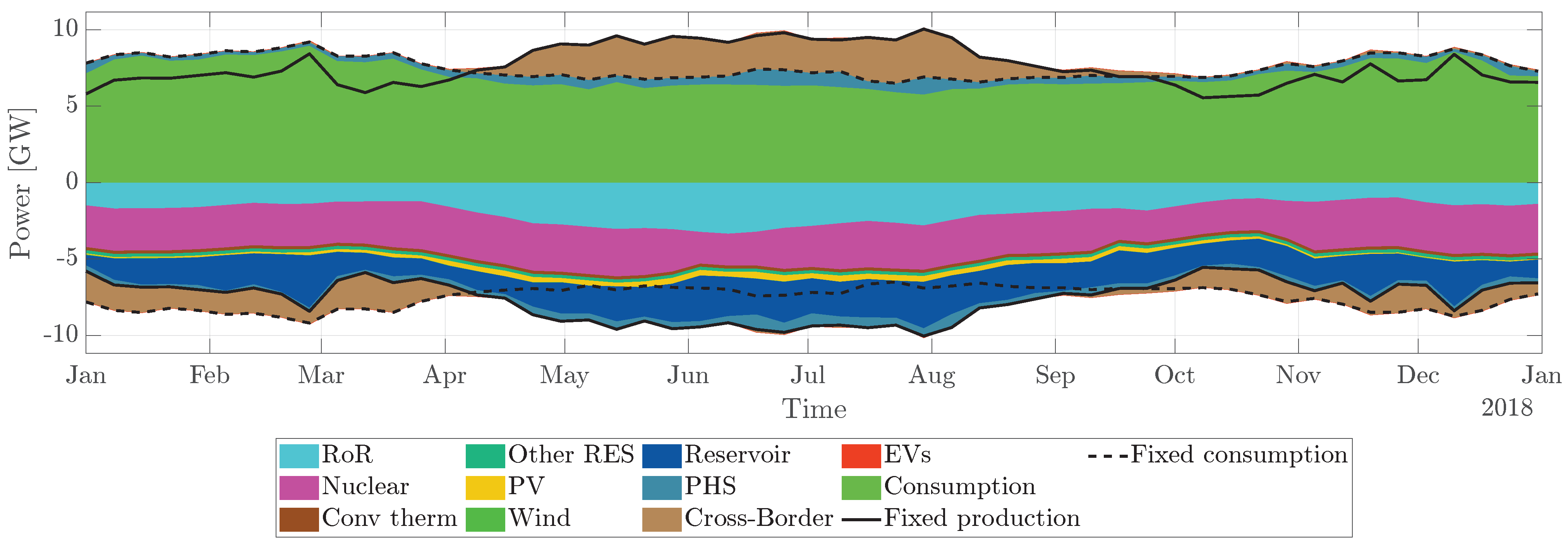
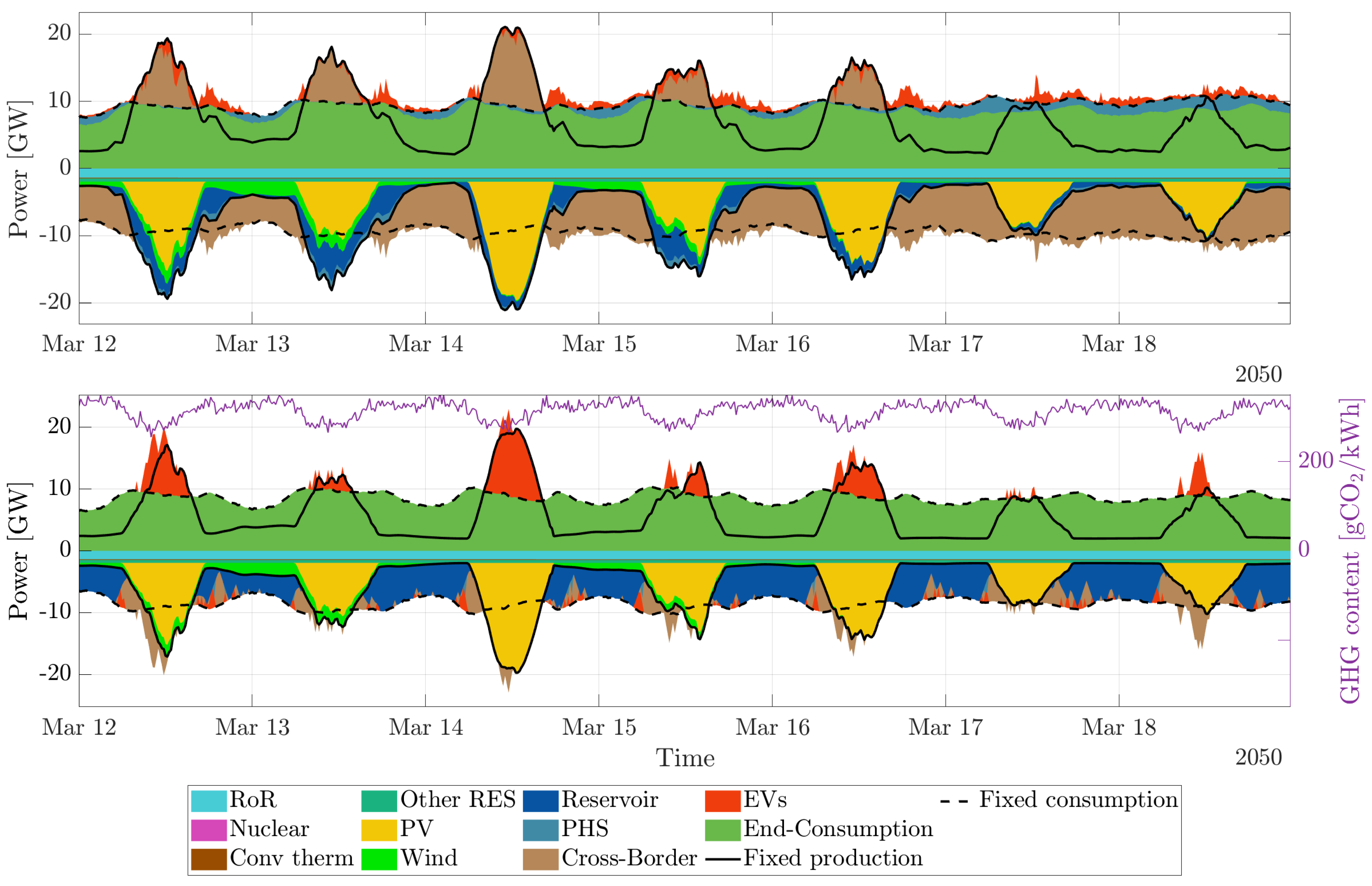
4.1. Impact of the Optimization on the Power Flows

Figure 3 shows the difference in power flows between the uncontrolled case (top) and the case when EVs, reservoirs, and PHS facilities are monitored together (bottom) for one week in March 2050 in the ZERO-EBM scenario with a horizon of one year. We can see the optimization shifting the charging of EVs towards the middle of the days (positive red values) when the sun is shining and the carbon content of the European grid is lower, to make use of electricity surpluses instead of exporting them. Reservoirs and small discharging operations from EVs are on the other hand avoiding GHG-intensive electricity imports in the evenings and overnights. This is, however, not enough to get a completely self-sufficient Swiss power system, and one can still observe some imports at times when the carbon content of the European grid is at its lowest, often in the mornings.

Due to the yearly optimization horizon, reservoirs are heavily utilized in March to cover the night demand, as there are only little surpluses of energy that could be stored in EV batteries—additionally to what they need during trips—or PHS facilities. Later in summer, larger surpluses of energy, mainly from solar-based electricity sources, allow for more V2G operations and less intensive reservoir utilization, as shown in Figure 4. The lack of surplus energy in March also explains why electricity storage in PHS facilities is circumvented over that period: since they present a lower round trip efficiency than bidirectional EVs, the optimization firstly charges energy through V2G, to decrease losses, after which no additional electricity is left in the system to pump water in PHS facilities.

4.2. From Uncontrolled to Bidirectional EV Charging

The tendency of uncontrolled charging to put further strain on the power grid and worsening the evening demand peak of the duck curve is demonstrated in Figure 5, where the average hourly (dis-)charging curve of EVs is shown for each season of 2050 under UC, V1G, and V2G for the ZERO-EBM scenario. In these plots, the hydropower plants are not optimized and follow their historical pattern. Once controlled charging (V1G) is introduced, the optimization generally shifts the bulk of the EV energy consumption to around noon, taking advantage of the high share of solar-based renewable energy in this scenario. This effect is less marked in summer because of electricity surpluses being available most of the day to charge the vehicles without relying on imports, mostly coming from hydro power plants.

Widespread adoption of bidirectional charging (V2G) allows to store surplus energy—besides what is needed for trips—in EV batteries, mainly solar energy over noon, which is then is fed back to the grid to support evening and nighttime demand. This has a great potential to mitigate the duck curve, simultaneously shifting additional demand to periods of high electricity production and reducing the net demand in the evening with discharging operations. We can observe a larger potential for V2G in transition seasons, where Switzerland alternates between over- and underproduction situations that can be exploited by the optimization. V2G has the least impact in summer since surpluses are almost always available, and Switzerland becomes a large net exporter of electricity because the storage capacities are full. Indeed, the lower energy demand in summer is covered by solar and hydropower—following their historical production profile—during the days and evenings, with EVs only needing to supply electricity during the night, discharging energy from 11 pm to 6 am. On the contrary, the potential of V2G is limited in winter due to the low domestic energy production, stemming from the high share of intermittent renewable energy sources, and the larger demand ensuing from the electrification of the heating sector. This shows that energy systems with a large share of RES cannot solely rely on V2G to avoid energy exchanges with connected markets, even when millions of EVs, hence a large storage capacity, are available.

The situation in the BAU scenario is very similar, but with less impact of control algorithms because of the much smaller exploitable discrepancies between the electricity production and consumption, due to the larger conventional thermal baseload. Likewise, reducing the number of EVs on the roads (NEP) leads to smaller charging and discharging magnitudes but identical behaviors of electric vehicles under different control strategies. Thus, in all scenarios, V1G shifts the peak towards noon, and V2G emphasizes this trend to furthermore support the power system overnight.

4.3. Reductions of Imported GHG Emissions

The potential of controlling EVs, reservoirs, and/or PHS facilities to mitigate GHG emissions stemming from power imports is demonstrated in Figure 6. Possible relative reductions in imported GHG-intensive electricity compared to the uncontrolled base case are shown. In plots (a–e), we compare the mitigation potential of all the participants in a yearly optimization and with a high number of EVs (EBM). With plots (f–j), one can either assess the impact of changing the optimization horizon or the number of EVs for each control strategy. Note that we are only interested in relative reductions here, but the total amount of imported emissions is larger in the BAU or EBM scenarios, because of the lower production and higher consumption of electricity, respectively, making Switzerland more reliant on neighboring countries and increasing the amount of GHG-intensive electricity imports. We can furthermore observe that EV control algorithms generally present low potential in the near future because the very low number of EVs in the system cannot significantly influence the number of emissions, but we then see a rise in mitigation potential from 2030 on, once the aggregated energy and power capacity of EV batteries becomes meaningful. In other words, energy systems will have to rely on other storage technologies in the coming years, such as hydro-based facilities in Switzerland, before V1G or V2G solutions start to have a comparable impact.

In general, the larger daily and yearly discrepancies between the electricity demand and production stemming from the bigger share of solar-based generation in the ZERO scenario provide control algorithms with more possibilities to avoid imports. This is further emphasized for V2G and PHS since they can charge surpluses of energy during the day and discharge them later to cover deficits (b,c). On the other hand, reservoirs are less sensitive to daily discrepancies, since natural water inflows “recharge” them, and they can leverage longer-term storage operations, retaining water until the grid needs the most support in both energy scenarios (d). However, their mitigation potential is firstly decreasing in 2030 before slowly rising again, mainly due to the electricity deficits expected after the nuclear phase-out (Figure 2). This lack of domestic production will indeed increase the reliance of Switzerland on neighboring countries, leading to imports even in the best case and leaving less flexibility for control strategies.

Focusing on the ZERO scenario in the first line of plots, we can observe that controlling PHS facilities, reservoirs, and V2G individually can reduce emissions by 33% to 40% in 2050. When we optimize the three together, we can attain a mitigation potential of almost 60%, with the reservoirs engaging in more long-term storage operations and V2G taking advantage of daily electricity supply and demand discrepancies (e). We thus see the combined mitigation potential following a similar path to the one of reservoirs, with V2G and PHS providing additional reduction possibilities and emphasizing the difference between the BAU and ZERO scenario. This is confirmed by (i), which shows a large drop in the mitigation potential of dams when the optimization horizon is shortened to a week, proving their ability to engage in long-term operations. Similarly, the possible reductions of emissions using reservoirs, PHS and V2G together plummet to about 40% in 2050 in the ZERO-EBM scenario when reservoirs cannot participate in long-term storage (j). Note that V2G alone could mitigate around 35% of emissions, even with a weekly horizon, showing how critical the horizon is for reservoirs. Since a full-year optimization with perfect forecasts is not realistic, we can thus conclude that V2G shows the greatest potential once the aggregated EV battery capacity can rival the potential of PHS facilities, particularly in a large intermittent renewable energy production scenario.

Both V1G and V2G are, on the other hand, not sensitive to the optimization horizon, confirming that they profit from daily discrepancies and do not engage in longer-term operations. They are, however, impacted by the number of EVs on the road, with V1G taking more advantage of an increased number of EVs (from NEP (f) to EBM (a)) than V2G (g,b). This comes from the fact that V1G can only shift the demand from EVs and thus influence imports directly related to vehicles, while V2G can additionally shift electricity production to support the grid, thereby also affecting imports not linked to EVs. As the number of vehicles grows, more and more emissions can be linked to the additional demand coming from EVs, and V1G can shift it to reduce GHG-intensive imports, increasing its mitigation potential. In the case of V2G, however, we see no significant difference in the reduction of emissions from NEP to EBM each year of the horizon, indicating that V2G reaches its maximum potential already with a low number of EVs. Remarkably, this means we would only need a small part of EV owners to participate in grid support operations to attain the maximum potential of V2G before the benefits saturate, making additional participants redundant. Additionally, this saturation also indicates that we cannot expect V2G to single-handedly tackle the mismatch between the production and consumption of electricity.

4.4. Impact on the Net Demand Curve

The net demand curve of a system, where the domestic electricity production is subtracted from the demand, quantifies the need for power import or export at each point in time. In Figure 7, we investigate the impact of the performed GHG-intensive imports minimization on the Swiss net demand curve, to analyze the reliance of Switzerland on neighboring countries. The average hourly imports and exports are plotted for the different control strategies in each season in both energy scenarios in 2050, in the EBM scenario, and with an optimization horizon of one year.

Using any storage technology to reduce imported GHG emissions generally flattens the net demand curve, with V2G showing the most marked changes, shifting the demand towards noon and feeding energy back to the grid at night to avoid GHG-intensive electricity imports. The biggest impacts are obtained in transition seasons, where control strategies take advantage of the increased daily energy production and consumption discrepancies to decrease the reliance on imports from neighboring countries during the night. Remarkably, the net demand curve is reversed in some cases, especially in winter and autumn, due to the desired GHG-intensive imports minimization, which prompts the model to import more electricity around noon, when the GHG profile of the European grid is lower.

In a scenario with large penetration of solar-based electricity production (ZERO), increasing amounts of energy surpluses are to be expected in spring and summer, and Switzerland should take advantage of them with further mitigation strategies. Indeed, this energy will otherwise have to be curtailed, as neighboring countries will face a similar situation of overproduction of electricity over noon. Nevertheless, control strategies are able to erase the need for imports overnight in summer and decrease them significantly in spring. However, in both energy scenarios, Switzerland will stay a net electricity importer in winter and a net exporter in summer, even with the combined effort of EVs, reservoirs, and PHS facilities (green curves). The country will thus remain dependent on its neighbors for energy exchanges in the future, even with control strategies aiming at minimizing GHG-intensive imports.

4.5. Analysis of the Net Transfer Capacity

Similarly to previous works on the Swiss power system [8,25,26], cross-border exchange capacities prove to become main bottlenecks over the years, threatening Switzerland’s security of supply. A summary of the problem can be found in Figure 8 for the ZERO-EBM scenario with an optimization horizon of one year. This plot compares the needed power import or export at each time step to current cross-border capacities and planned extensions, as projected by the Swiss TSO in 2025 [49]. Even these increased net transfer capacities might not be sufficient in future years if Switzerland follows its intention to install a large share of intermittent renewable energy sources without complementary control strategies.

Towards 2050, the control of PHS facilities alone will not be enough to decrease imports to 2018 levels, but it will suffice for the planned extensions, contrary to V1G. Nonetheless, in general, different control strategies prove to be able to reduce the magnitude imports below the current bounds, which will ensure that Switzerland is able to meet its domestic demand at all times. It is however noteworthy that no control strategy is able to mitigate exports to feasible magnitudes in the coming years without curtailment of energy surpluses. However, exports were not constrained in this study and other control algorithms might be able to mitigate this issue to some extent as well.

The situation is similar in the BAU scenario, with V1G and the control of PHS facilities able to reduce imports to lie beneath the projected extension to the NTC 2025 limit, but not below the current bounds, contrary to the other control strategies, as shown in Appendix D. The smaller share of intermittent renewable electricity production in that case would, however, sharply decrease the bottleneck issue in export capacity.

4.6. EV Battery Degradation Analysis

To complete our analysis and balance the positive impacts of EV control strategies, we investigate the effects of the optimization on the degradation of EV batteries, as a consequence of their different usage in UC, V1G, or V2G. We use a rainflow algorithm to count the number and depth of cycles the batteries undergo during the simulations [50]. A Wöhler curve of lithium-ion batteries is then used to evaluate the cyclic degradation of the batteries [51]. The resulting degradation for the three charging strategies in 2050 in the ZERO scenario can be found in Figure 9, where the cycle lives of the 100 EVs are described.We can then compare the cycle life to the calendar life of lithium-ion batteries, which represents how a battery degrades with time when it remains inactive or is minimally used. Finally, the life of a battery is commonly defined as the minimum value between its calendar and cycle life.

In Figure 9, we can see that most cars present a lower calendar than cyclic life in the UC and V1G cases, thereby implying that these charging behaviors do not severely impact battery lives. However, many EVs show lower cycle lives under V2G operations in the NEP scenario (left), indicating that the increased number of cycles used to support the grid can be detrimental in terms of degradation. Remarkably, cycle lives rise when more cars can engage in bidirectional charging operations (right), suggesting that individual EVs get less used when more vehicles are available for V2G schemes. This favorably aligns with the observation from Section 4.3 that V2G reaches its full potential before a high number of EVs is attained.

Furthermore, this means one could limit the cyclic degradation of EV batteries that engage in V2G operations to not go below their calendar life and still be able to significantly reduce the amount of imported GHG emissions in the EBM scenario. Interestingly, this proves that V2G might not have any negative impact on the lives of EV batteries if there are enough participants in the market, thereby lifting one of the main barriers towards widespread adoption of the technology. Hence, while the full potential of V2G to reduce imported GHG emissions can be reached with a low number of EVs participating fully, additional participants, while not being able to bring much further support to the grid, would reduce the degradation of individual batteries, and hence the costs of V2G operations.

5. Conclusions

In this work, we evaluated the impacts of electric vehicles under uncontrolled, controlled, and bidirectional charging on energy systems with a high share of renewable energy production, looking at how they could compete or interplay with other electricity storage technologies. Using Switzerland as a case study, we investigated the potential of EVs, reservoirs, and pumped-hydro storage facilities to decrease the amount of GHG-intensive electricity imports in different scenarios.

Leveraging the high expected solar-based electricity production in the coming years, controlled charging of EVs shifts their energy demand away from evening peaks to maximize self-consumption of electricity around noon. When bidirectional charging is enabled, additional electricity surpluses can be stored in EV batteries and fed back to the grid in critical periods to avoid further GHG-intensive imports.

In a scenario with a high share of intermittent renewable energy production, V2G shows potential to reduce the amount of imported GHG emissions by around 35% over the year 2050, similarly to reservoirs and PHS facilities. When these three storage technologies are combined, reductions of 60% can be attained, with reservoirs taking part in longer-term operations and EVs dealing with daily discrepancies between the production and consumption of electricity. When the optimization horizon is shortened from a year to a week, however, reservoirs lose a large part of their mitigation potential, while V2G keeps comparable performance to reduce emissions. Nonetheless, EVs firstly need to reach a sufficient aggregated capacity and the electricity production from renewable energy sources has to significantly increase before V2G becomes interesting. Thereafter, EVs will be able to engage in bidirectional charging operations needed to cover the increasing daily discrepancies between the production and consumption of electricity. Until that point is reached, however, power systems will have to rely on other installed storage technologies, such as hydropower facilities, to act as buffers to avoid GHG-intensive electricity imports.

In all cases, our results suggest that Switzerland will remain a net importer of electricity in winter and a net exporter in summer since no control strategy will be able to fully flatten its net demand curve. Nonetheless, controlling EVs, reservoirs, or, to some extent, PHS facilities, could decrease the magnitude of electricity imports to satisfy cross-border transfer capacities. However, congestion limits might remain a problem for electricity exports if we want to avoid curtailment of solar power surpluses in summer. Alternatively, such surpluses could be further exploited through seasonal storage, but this would call for the installation of long-term storage facilities, such as hydrogen and/or synthetic natural gas.

Remarkably, our analyses point towards a saturation of the mitigation potential of V2G, showing that this technology cannot be expected to single-handedly erase the need for GHG-intensive electricity imports. In particular, it cannot leverage seasonal storage, which is needed to counter the growing seasonal discrepancies between the production and consumption of electricity. However, if increasing the number of vehicles participating in V2G operations does not allow for better support to the grid, it benefits individual EVs, as they are less heavily used by the system, which in turn has a positive impact on their battery lives.

Further studies on the subject should investigate what the tipping points for V2G are, i.e., how many participants are required to either reach this maximum potential or ensure that individual battery lives are not impacted. Moreover, the optimization could be enhanced, for example, using a receding horizon strategy, designing more detailed and marginal GHG emissions models, or incorporating a limit on battery degradation in the objective when V2G is considered as a control strategy. Finally, it would be interesting to include different energy sources and emission models in the framework to assess how the behavior of the various actors changes.

References

1. United Nations Framework Convention on Climate Change (UNFCCC). Paris Agreement to the United Nations Framework Convention on Climate Change. 2015. Available online: https://unfccc.int/process-and-meetings/the-paris-agreement/the-paris-agreement (accessed on 5 May 2021).
2. Prognos AG and INFRAS AG and TEP Energy GmbH and Ecoplan AG. ENERGIEPERSPEKTIVEN 2050+ Kurzbericht. 2020. Available online: https://www.newsd.admin.ch/newsd/message/attachments/64121.pdf (accessed on 12 May 2021).
3. Coignard, J.; Saxena, S.; Greenblatt, J.; Wang, D. Clean vehicles as an enabler for a clean electricity grid. Environ. Res. Lett. 2018, 13, 054031. [Google Scholar] [CrossRef]
4. Rüdisüli, M.; Teske, S.L.; Elber, U. Impacts of an Increased Substitution of Fossil Energy Carriers with Electricity-Based Technologies on the Swiss Electricity System. Energies 2019, 12, 2399. [Google Scholar] [CrossRef] [Green Version]
5. Schlömer, S.; Bruckner, T.; Fulton, L.; Hertwich, E.M.A.; Perczyk, D.; Roy, J.; Schaeffer, R.; Sims, R.; Smith, P.; Wiser, R. Annex III: Technology-Specific Cost and Performance Parameters; Cambridge University Press: Cambrige, UK, 2014. [Google Scholar]
6. Ding, N.; Duan, J.; Xue, S.; Zeng, M.; Shen, J. Overall review of peaking power in China: Status quo, barriers and solutions. Renew. Sustain. Energy Rev. 2015, 42, 503–516. [Google Scholar] [CrossRef]
7. Korpås, M.; Wolfgang, O. Norwegian pumped hydro for providing peaking power in a low-carbon European power market—Cost comparison against OCGT and CCGT. In Proceedings of the 2015 12th International Conference on the European Energy Market (EEM), Lisbon, Portugal, 19–22 May 2015; pp. 1–5. [Google Scholar] [CrossRef] [Green Version]
8. Dujardin, J.; Kahl, A.; Kruyt, B.; Bartlett, S.; Lehning, M. Interplay between photovoltaic, wind energy and storage hydropower in a fully renewable Switzerland. Energy 2017, 135, 513–525. [Google Scholar] [CrossRef]
9. International Energy Agency (IEA). Global EV Outlook 2021. 2021. Available online: https://www.iea.org/reports/global-ev-outlook-2021?mode=overview (accessed on 19 May 2021).
10. Boudina, R.; Wang, J.; Benbouzid, M.; Yao, G.; Zhou, L. A Review on Stochastic Approach for PHEV Integration Control in a Distribution System with an Optimized Battery Power Demand Model. Electronics 2020, 9, 139. [Google Scholar] [CrossRef] [Green Version]
11. Ehsani, M.; Falahi, M.; Lotfifard, S. Vehicle to grid services: Potential and applications. Energies 2012, 5, 4076–4090. [Google Scholar] [CrossRef] [Green Version]
12. Zhang, C.; Greenblatt, J.B.; MacDougall, P.; Saxena, S.; Prabhakar, A.J. Quantifying the benefits of electric vehicles on the future electricity grid in the midwestern United States. Appl. Energy 2020, 270, 115174. [Google Scholar] [CrossRef]
13. Bhandari, V.; Sun, K.; Homans, F. The profitability of vehicle to grid for system participants-A case study from the Electricity Reliability Council of Texas. Energy 2018, 153, 278–286. [Google Scholar] [CrossRef]
14. Fernandes, C.; Frías, P.; Latorre, J.M. Impact of vehicle-to-grid on power system operation costs: The Spanish case study. Appl. Energy 2012, 96, 194–202. [Google Scholar] [CrossRef]
15. Kobashi, T.; Yoshida, T.; Yamagata, Y.; Naito, K.; Pfenninger, S.; Say, K.; Takeda, Y.; Ahl, A.; Yarime, M.; Hara, K. On the potential of “Photovoltaics+ Electric vehicles” for deep decarbonization of Kyoto’s power systems: Techno-economic-social considerations. Appl. Energy 2020, 275, 115419. [Google Scholar] [CrossRef]
16. Brinkel, N.; Schram, W.; AlSkaif, T.; Lampropoulos, I.; van Sark, W. Should we reinforce the grid? Cost and emission optimization of electric vehicle charging under different transformer limits. Appl. Energy 2020, 276, 115285. [Google Scholar] [CrossRef]
17. World Nuclear Association. Nuclear Power in Switzerland. 2021. Available online: https://world-nuclear.org/information-library/country-profiles/countries-o-s/switzerland.aspx (accessed on 5 May 2021).
18. Swiss Federal Office of Energy (SFOE). Nuclear Energy. 2020. Available online: https://www.bfe.admin.ch/bfe/en/home/supply/nuclear-energy.html (accessed on 11 February 2021).
19. Federal Office for the Environment (FOEN). Greenhouse Gas Inventory: Evolution of Switzerland’s Greenhouse Gas Emissions Since 1990. 2020. Available online: https://www.bafu.admin.ch/bafu/en/home/topics/climate/state/data/greenhouse-gas-inventory.html (accessed on 11 February 2021).
20. Federal Statistical Office (FSO). Road Vehicles—Stock, Level of Motorisation. 2020. Available online: https://www.bfs.admin.ch/bfs/en/home/statistics/mobility-transport/transport-infrastructure-vehicles/vehicles/road-vehicles-stock-level-motorisation.html (accessed on 11 February 2021).
21. Kirchner, A.; Bredow, D.; Ess, F.; Grebel, T.; Hofer, P.; Kemmler, A.; Ley, A.; Piégsa, A.; Schütz, N.; Strassburg, S.; et al. Energy Perspectives, Die Energieperspektiven für die Schweiz bis 2050; Prognos AG: Basel, Switzerland, 2012. [Google Scholar]
22. Rüdisüli, M.; Bach, C.; Bauer, C.; Beloin-Saint-Pierre, D.; Elber, U.; Georges, G.; Limpach, R.; Pareschi, G.; Kannan, R.; Teske, S.L. Prospective life-cycle assessment of greenhouse gas emissions of electricity-based mobility options. Manuscr. Submitt. Appl. Energy 2021, submitted. [Google Scholar]
23. Swiss Federal Office of Energy (SFOE). Electricity Statistics. 2020. Available online: https://www.bfe.admin.ch/bfe/en/home/supply/statistics-and-geodata/energy-statistics/electricity-statistics.html (accessed on 11 February 2021).
24. Bundesversammlung der Schweizerischen Eidgenossenschaft (BSE). Bundesgesetz über die Reduktion der CO2-Emissionen. 2013. Available online: https://fedlex.data.admin.ch/filestore/fedlex.data.admin.ch/eli/cc/2012/855/20180101/de/pdf-a/fedlex-data-admin-ch-eli-cc-2012-855-20180101-de-pdf-a.pdf (accessed on 12 May 2021).
25. Bartlett, S.; Dujardin, J.; Kahl, A.; Kruyt, B.; Manso, P.; Lehning, M. Charting the course: A possible route to a fully renewable Swiss power system. Energy 2018, 163, 942–955. [Google Scholar] [CrossRef]
26. Abrell, J.; Eser, P.; Garrison, J.B.; Savelsberg, J.; Weigt, H. Integrating economic and engineering models for future electricity market evaluation: A Swiss case study. Energy Strategy Rev. 2019, 25, 86–106. [Google Scholar] [CrossRef]
27. Muratori, M. Impact of uncoordinated plug-in electric vehicle charging on residential power demand. Nat. Energy 2018, 3, 193–201. [Google Scholar] [CrossRef]
28. Forrest, K.E.; Tarroja, B.; Zhang, L.; Shaffer, B.; Samuelsen, S. Charging a renewable future: The impact of electric vehicle charging intelligence on energy storage requirements to meet renewable portfolio standards. J. Power Sources 2016, 336, 63–74. [Google Scholar] [CrossRef]
29. Uddin, K.; Dubarry, M.; Glick, M.B. The viability of vehicle-to-grid operations from a battery technology and policy perspective. Energy Policy 2018, 113, 342–347. [Google Scholar] [CrossRef]
30. Rüdisüli, M.; Romano, E.; Eggimann, S.; Patel, M. Marginal GHG content of electricity used for various demand and supply scenarios in Switzerland. Manuscr. Submitt. Energy Policy 2021, submitted. [Google Scholar]
31. Staffell, I.; Pfenninger, S. Using bias-corrected reanalysis to simulate current and future wind power output. Energy 2016, 114, 1224–1239. [Google Scholar] [CrossRef] [Green Version]
32. Bundesamt für Energie (BFE). Schweizerische Elektrizitätsstatistik 2018. Available online: https://www.bfe.admin.ch/bfe/de/home/versorgung/statistik-und-geodaten/energiestatistiken/elektrizitaetsstatistik.html (accessed on 4 August 2021).
33. Swissgrid. Produktion und Verbrauch. 2020. Available online: https://www.swissgrid.ch/de/home/operation/grid-data/generation.html#downloads (accessed on 5 May 2021).
34. Beer, M. Abschätzung des Potenzials der Schweizer Speicherseen zur Lastdeckung bei Importrestriktionen. Z. Energiewirtschaft 2018, 42, 1–12. [Google Scholar] [CrossRef]
35. Pareschi, G.; Georges, G.; Boulouchos, K. Assessment of the Marginal Emission Factor associated with Electric Vehicle Charging. In Proceedings of the 1st E-Mobility Power System Integration Symposium, Berlin, Germany, 23 October 2017. [Google Scholar] [CrossRef]
36. Pareschi, G.; Küng, L.; Georges, G.; Boulouchos, K. Are travel surveys a good basis for EV models? Validation of simulated charging profiles against empirical data. Appl. Energy 2020, 275, 115318. [Google Scholar] [CrossRef]
37. Bundesamt für Raumentwicklung (ARE). Mikrozensus Mobilität und Verkehr. 2015. Available online: https://www.are.admin.ch/are/de/home/verkehr-und-infrastruktur/grundlagen-und-daten/verkehrsverhalten.html (accessed on 5 May 2021).
38. Nicholas, M.; Wappelhorst, S. Regional Charging Infrastructure Requirements in Germany through 2030, White Paper. 2020. Available online: https://theicct.org/publications/regional-charging-infra-germany-oct2020 (accessed on 4 August 2021).
39. de Tena Costales, L.D. Large Scale Renewable Power Integration with Electric Vehicles; OPUS - Online Publikationen der Universität Stuttgart: Stuttgart, Germany, 2014. [Google Scholar] [CrossRef]
40. Bundesamt für Landestopografie Swisstopo (FOT). Ladestationen für Elektroautos. 2019. Available online: https://www.ich-tanke-strom.ch (accessed on 5 May 2021).
41. Schram, W.; Brinkel, N.; Smink, G.; van Wijk, T.; van Sark, W. Empirical Evaluation of V2G Round-trip Efficiency. In Proceedings of the 2020 International Conference on Smart Energy Systems and Technologies (SEST), Istanbul, Turkey, 7–9 September 2020; pp. 1–6. [Google Scholar] [CrossRef]
42. International Renewable Energy Agency (IRENA). Innovative Ancillary Services: Innovation Landscape Brief. 2019. Available online: https://www.irena.org/-/media/Files/IRENA/Agency/Publication/2019/Feb/IRENA_Innovative_ancillary_services_2019.pdf?la=en&hash=F3D83E86922DEED7AA3DE3091F3E49460C9EC1A0 (accessed on 12 May 2021).
43. Vaya, M.G.; Andersson, G. Centralized and decentralized approaches to smart charging of plug-in vehicles. In Proceedings of the 2012 IEEE Power and Energy Society General Meeting, San Diego, CA, USA, 22–26 July 2012; pp. 1–8. [Google Scholar] [CrossRef]
44. Al-Ogaili, A.S.; Hashim, T.J.T.; Rahmat, N.A.; Ramasamy, A.K.; Marsadek, M.B.; Faisal, M.; Hannan, M.A. Review on scheduling, clustering, and forecasting strategies for controlling electric vehicle charging: Challenges and recommendations. IEEE Access 2019, 7, 128353–128371. [Google Scholar] [CrossRef]
45. Richardson, P.; Flynn, D.; Keane, A. Local versus centralized charging strategies for electric vehicles in low voltage distribution systems. IEEE Trans. Smart Grid 2012, 3, 1020–1028. [Google Scholar] [CrossRef]
46. MATLAB. MATLAB Version 9.10.0.1602886 (R2021a); The MathWorks Inc.: Natick, MA, USA, 2021. [Google Scholar]
47. Löfberg, J. YALMIP: A Toolbox for Modeling and Optimization in MATLAB. In Proceedings of the CACSD Conference, Taipei, Taiwan, 2–4 September 2004. [Google Scholar]
48. Gurobi Optimization LLC. Gurobi Optimizer Reference Manual. 2021. Available online: http://www.gurobi.com (accessed on 5 May 2021).
49. von Kupsch, B. Bericht zum Strategischen Netz 2025. 2015. Available online: https://www.swissgrid.ch/dam/swissgrid/projects/strategic-grid/sg2025-technical-report-de.pdf (accessed on 12 May 2021).
50. Xu, B.; Oudalov, A.; Ulbig, A.; Andersson, G.; Kirschen, D.S. Modeling of lithium-ion battery degradation for cell life assessment. IEEE Trans. Smart Grid 2016, 9, 1131–1140. [Google Scholar] [CrossRef]
51. Ecker, M.; Nieto, N.; Käbitz, S.; Schmalstieg, J.; Blanke, H.; Warnecke, A.; Sauer, D.U. Calendar and cycle life study of Li (NiMnCo) O2-based 18650 lithium-ion batteries. J. Power Sources 2014, 248, 839–851. [Google Scholar] [CrossRef]
52. Rienecker, M.M.; Suarez, M.J.; Gelaro, R.; Todling, R.; Bacmeister, J.; Liu, E.; Bosilovich, M.G.; Schubert, S.D.; Takacs, L.; Kim, G.K.; et al. MERRA: NASA’s modern-era retrospective analysis for research and applications. J. Clim. 2011, 24, 3624–3648. [Google Scholar] [CrossRef]
53. Molod, A.; Takacs, L.; Suarez, M.; Bacmeister, J. Development of the GEOS-5 atmospheric general circulation model: Evolution from MERRA to MERRA2. Geosci. Model Dev. 2015, 8, 1339–1356. [Google Scholar] [CrossRef] [Green Version]
54. Swiss Federal Office of Energy (SFOE). Stand der Wasserkraftnutzung 31.12.2019; Swiss Federal Office of Energy (SFOE): Bern, Switzerland, 2020. [Google Scholar]
55. Electric Vehicle Database. A Complete Overview of All Electric Vehicles in Europe. 2021. Available online: https://ev-database.org/ (accessed on 27 July 2021).
56. Auto-Schweiz. PW-Zulassungen nach Modellen. 2021. Available online: https://www.auto.swiss (accessed on 12 May 2021).
Figure 1. Average weekly electricity consumption (positive) and the corresponding production (negative) in Switzerland in 2018. Cross−border either reflects imports in winter when the production (continuous black line) cannot meet the demand (dotted line) or exports in summer when there are surpluses.
Energies 14 04812 g001
Figure 2. BAU and ZERO Electricity production and consumption scenarios, with the impact of EVs on the demand in the NEP and EBM scenarios. Note that the base demand includes the electricity consumption of PHS facilities.
Energies 14 04812 g002
Figure 3. Consumption (positive) and the corresponding production (negative) of electricity in Switzerland over one week in March in the ZERO−EBM scenario in 2050. The upper plot shows the situation if no control action is taken, while the lower one presents the impact of the combined control of EVs (V2G), reservoirs, and PHS facilities, as well as the carbon content of the imported electricity.
Energies 14 04812 g003
Figure 4. Weekly average electricity production from reservoirs in 2050 in the ZERO-EBM scenario, comparing the uncontrolled case and the case where the optimization is done over EVs, reservoirs, and PHS facilities.
Energies 14 04812 g004
Figure 5. Comparison of average charging profiles in the four seasons in 2050 in the ZERO−EBM scenario for uncontrolled charging, V1G, and V2G.
Energies 14 04812 g005
Figure 6. Potential of V1G, V2G, reservoirs, PHS, and the combination of three latter variables to reduce GHG emissions, compared to the case where none of them is controlled. In the top plots, the five control strategies are compared in the EBM scenario and with a yearly horizon. In the bottom ones, either the EV scenario is changed to NEP or the horizon is shortened to one week, depending on which case is more interesting.
Energies 14 04812 g006
Figure 7. Net demand curves of Switzerland in 2050 in the EBM scenario under both energy scenarios and different control strategies, where V1G was excluded for clarity as its impact, is less important.
Energies 14 04812 g007
Figure 8. Analysis of the exports (negative) and imports (positive) with the European grid over each year of the optimization and for the different control strategies, compared to the installed and projected Net Transfer Capacity in the ZERO−EBM scenario, where the quartiles are set at 25–75% and the whiskers represent 1.5 times the interquartile range.
Energies 14 04812 g008
Figure 9. Battery degradation analysis under the three different EV control algorithm in 2020 and in the ZERO scenario for both the lower and higher number of vehicles. A few outliers with extremely high cycle life have been left out for clarity.
Energies 14 04812 g009