Article

The Implementation of Multiple Linear Regression for Swimming Pool Facilities: Case Study at Jøa, Norway

1
Department of Civil and Environmental Engineering, NTNU Norwegian University of Science and Technology, 7491 Trondheim, Norway
2
COWI AS, 7436 Trondheim, Norway
3
SIAT NTNU—Centre for Sport Facilities and Technology, Department for Civil and Transport Engineering, NTNU Norwegian University of Science and Technology, 7491 Trondheim, Norway
4
Department of Energy and Process Engineering, NTNU Norwegian University of Science and Technology, 7491 Trondheim, Norway
5
Energy, Environment and Water Research Center, The Cyprus Institute, Aglantzia 2121, Cyprus
*
Author to whom correspondence should be addressed.
Energies 2021, 14(16), 4825; https://doi.org/10.3390/en14164825
Submission received: 28 June 2021 / Revised: 2 August 2021 / Accepted: 4 August 2021 / Published: 7 August 2021

Abstract

:
This paper presents a statistical model for predicting the time-averaged total power consumption of an indoor swimming facility. The model can be a powerful tool for continuous supervision of the facility’s energy performance that can quickly disclose possible operational disruptions/irregularities and thus minimize annual energy use. Multiple linear regression analysis is used to analyze data collected in a swimming facility in Norway. The resolution of the original training dataset was in 1 min time steps and during the investigation was transposed both by time-averaging the data, and by treating part of the dataset exclusively. The statistically significant independent variables were found to be the outdoor dry-bulb temperature and the relative pool usage factor. The model accurately predicted the power consumption in the validation process, and also succeeded in disclosing all the critical operational disruptions in the validation dataset correctly. The model can therefore be applied as a dynamic energy benchmark for fault detection in swimming facilities. The final energy prediction model is relatively simple and can be deployed either in a spreadsheet or in the building automation reporting system, thus the method can contribute instantly to keep the operation of any swimming facility within the optimal individual energy performance range.

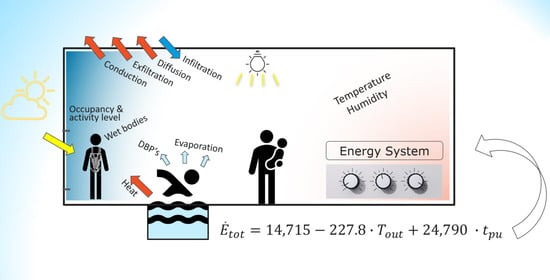
Graphical Abstract

1. Introduction

1.1. Background

The EU has defined a target for reducing GHG emissions by at least 40% by 2030 compared to 1990 levels [1]. Their long-term goal is defined as “no GHG emissions” by 2050 [2]. Increased energy efficiency in buildings is defined as an important tool for both the short term and long term [3]. One of the “key actions” in the Action Plan related to the 2030 framework is a “renovation wave” of the existing building stock [2].
Within the “renovation wave”, the European Commission recommends paying particular attention to energy-reducing refurbishment in types of buildings that support education and public health, such as schools and hospitals [2]. In swimming facilities, which support education and public health, the potential for energy reduction is considerable [4] and the literature associates these facilities with high specific energy use [5] and a large dispersion in energy use. The specific energy use ranges from 400 kWh/(m 2 · a) to almost 1600 kWh/(m 2 · a) [6,7,8,9]. This can be partially explained by the variations in age, technology and the different maintenance routines [7], but the numbers also represent a large energy saving potential [7]. Regarding the building stock of swimming facilities in Norway [6], the overall excessive energy use is estimated to be 28%. This provides a considerable incentive for improvement initiatives.

1.2. Motivation

Since the energy consumption of any building is highly dependent on the operational phase [10], particular attention has to be given to providing optimal operation [11]. Here, both behavioral and operational management are important [12]. It is crucial to emphasize the importance of well-trained and qualified operating personnel [13], especially in buildings with extensive technical installations like swimming facilities [13]. However, this is not always the case [14], and even with skilled operating staff, it is a considerable task to run a facility that has satisfactory performance. In the case of non-skilled operating staff, the performance of the facility is vulnerable if there is improper operation and possible excessive energy use and low indoor environmental quality. The complexity of the operation increases if there are more and more technical components [15]. In addition, during the operation phase, such factors will degrade the building and the technical systems, and the performance of the building will be lower than when it was commissioned [16]. This may lead to a poor indoor environment and increase the energy use. For buildings with extensive technical systems, such as swimming facilities, multiple operational interruptions may conceal other malfunctions and make it difficult for the operating staff to find them. The result is a building with low overall performance compared to the design level. This means that there is a need for strict holistic control and a supervision system for the performance of the building.
Ruparathna et al. [17] proposed a rating system for public buildings based on a level of service (LOS) index. This index is a qualitative measure that is traditionally used to compare the quality of motor vehicle traffic services. When applied to public buildings, the LOS index indicates the level of operational performance provided to building users, society and the environment, based on the assessment of the defined performance indicators in the building. For the operating staff, this kind of rating system can be applied as a useful tool if it is used as a continuous reporting system for the performance of the building. With the implementation of adequate performance indicators, this kind of system will contribute to keeping the technical installations “on track” as a lifetime commissioning system and a tool for fault diagnosis.
For swimming facilities, the number of performance indicators may be considerable and some are impossible to track directly in real time, for example, the level of some airborne disinfection by-products. Ruparathna et al. [17] implemented a set of 22 performance indicators in their case study, including measures like user satisfaction, indoor environmental quality, water quality and energy use, among others. Saleem et al. [18] investigated the choice of performance indicators for aquatic centers in Canada, and proposed a set of 63 indices, including water quality, indoor environmental quality, energy efficiency and user satisfaction.
Energy efficiency is an important aspect in these rating systems and is considered the most important criterion in sustainability rating systems as well as the least achieved [19]. This underlines the importance of a strict system for monitoring the energy performance along with the main functions of the building. Due to the large internal energy flow in swimming facilities, this is even more important because of the increased probability of operational faults and increased energy use.

1.3. Theoretical Background

Continuous assessment of building energy performance is a process of analyzing residuals. Here, the residual is the difference between the monitored energy use and the prediction of the expected energy use of a dynamic benchmarking system. Contrary to “snapshot” rating systems, such as energy labeling of buildings [20] or documentation for fulfilling the passive house standard [21,22], a dynamic benchmarking system depicts the continuous energy performance of the facility.
The prediction of the expected energy use is a complex task which depends on a large set of variables and parameters. The task should preferably be solved in a way which could easily be implemented in existing facilities and control systems. It should also be easy to adapt and be transparent for the operating staff. The importance of easy implementation is related to the increasing climate threat which can also be found in the short-term goal defined as the EU 2030 GHG reduction goal [1].
As they are different from other building types, swimming facilities are characterized by complex energy systems required to maintain appropriate conditions in the swimming hall and pool(s) and provide suitable water quality. Swimming halls are facilities with complex and energy-intensive technical systems [23], with several interacting subsystems. Figure 1 illustrates the extent of the technical systems and how they are connected internally and to external variables. These systems provide functions like fresh air supply, air heating, dehumidification, water heating and water treatment. The thermal and electric power/energy consumption levels of the different systems are logged in the building automation system.
The task of predicting the energy use in swimming facilities is complex due to constantly fluctuating variables such as evaporation of water from the pool and surrounding surfaces, the required amount of makeup water and the filter flushing intervals. Energy prediction has been treated in several studies where methods regarding outdoor and indoor swimming facilities have been presented.

1.4. Energy Prediction Methods

The energy prediction methods include physical/engineering methods as well as statistical and artificial intelligence methods [24]. Lu et al. [25] addressed the design and analysis stage and proposed a physical model for a sports facility. Despite the challenge related to the required numbers of parameters, the model performed with a coefficient of correlation ( R 2 ) of 0.934. Westerlund et al. [26] showed that the engineering approach for estimating annual energy use gave satisfactory results in swimming facilities as well. The results from this study, with a prosaic and simple technical structure, illustrates the importance of heat recovery, where evaporation dominates the energy demand. The same observation was also revealed in the study by Lovell et al. [27] where an engineering model for the prediction of thermal performance for an outdoor Olympic swimming pool in Australia was developed. The model was based on the heat balance and performed with an accuracy of 67% of the predicted heating capacities. This was within a range of ±100 kW, which proved to be the most accurate model compared to other equivalent models. The study confirmed that evaporation dominated the energy demand of an outdoor swimming facility. The same physical and empirical equations are also applied in building performance simulation tools such as TRNSYS [28], ESP-R [29] and IDA ICE [30], among others. Mančić et al. [31] determined the energy losses for a pool hall and pool, and later the optimal configuration of a polygeneration system [32], by modeling the system via physical and empirical equations in TRNSYS. Moreover, Duverge and Rajagopalan [33] investigated the energy and water performance of an aquatic center in Australia. They modeled the facility with the BPS tool EnergyPlus and recommended both solar heating and the use of vacuum filters in their study.
Yuce et al. [34] presented an artificial neural network approach for predicting the energy consumption and thermal comfort in an indoor swimming facility. The prediction was an application for an optimization-based control system for swimming facilities. Kampel et al. [35] proposed a statistical model for predicting the annual energy use of swimming facilities. It was developed through a multiple linear regression (MLR) analysis, and its purpose was to establish a tool for calculating energy performance indicators for the benchmarking of swimming facilities. In addition, the MLR method was also applied in the study by Duverge et al. [36]. One of the outcomes was that the usable floor area and the number of visitors were among the most influential variables for annual energy use.
While the simulation tools based on physical models and artificial neural networks, with different topologies and learning algorithms, can provide useful insights and efficiently predict target values, both frameworks are computationally costly and need case base adaptation. In the context of the practical use and implementation of energy prediction features among existing buildings, MLR has the potential to be in the middle ground with respect to computational cost and the opportunity to adapt it to the different target cases. MLR represents an easy-to-follow statistical method [37] which can explain a dependent variable, using multiple independent variables, but does not require in-depth knowledge of physical processes or training algorithms. It is easy to develop and implement [38] and is widely used in the prediction of energy use. For example, Safa et al. [39] presented a method to predict energy use in office buildings for the purpose of energy auditing. The study showed the capacity of simple models where the final regression model was based on outdoor temperature and occupancy with a monthly resolution. The model performed well with acceptable error, when assessing each of the four buildings in the study individually. Catalina et al. [40] developed a regression model for predicting the monthly space heating demand for residential buildings while another approach developed a generic equation of three variables for predicting the heating demand in apartments blocks [41]. The MLR method has also been applied with success in energy forecasting for swimming pool buildings [38,39].
The objective of this paper is to investigate and propose a method for energy prediction in swimming facilities, based on the MLR method. This approach has considerable potential for reducing the annual energy demand of both existing and new buildings by making the operating staff conscious of the performance of the building in relation to the design level. Buildings are only sustainable if they are operated and maintained properly [15].

2. Method

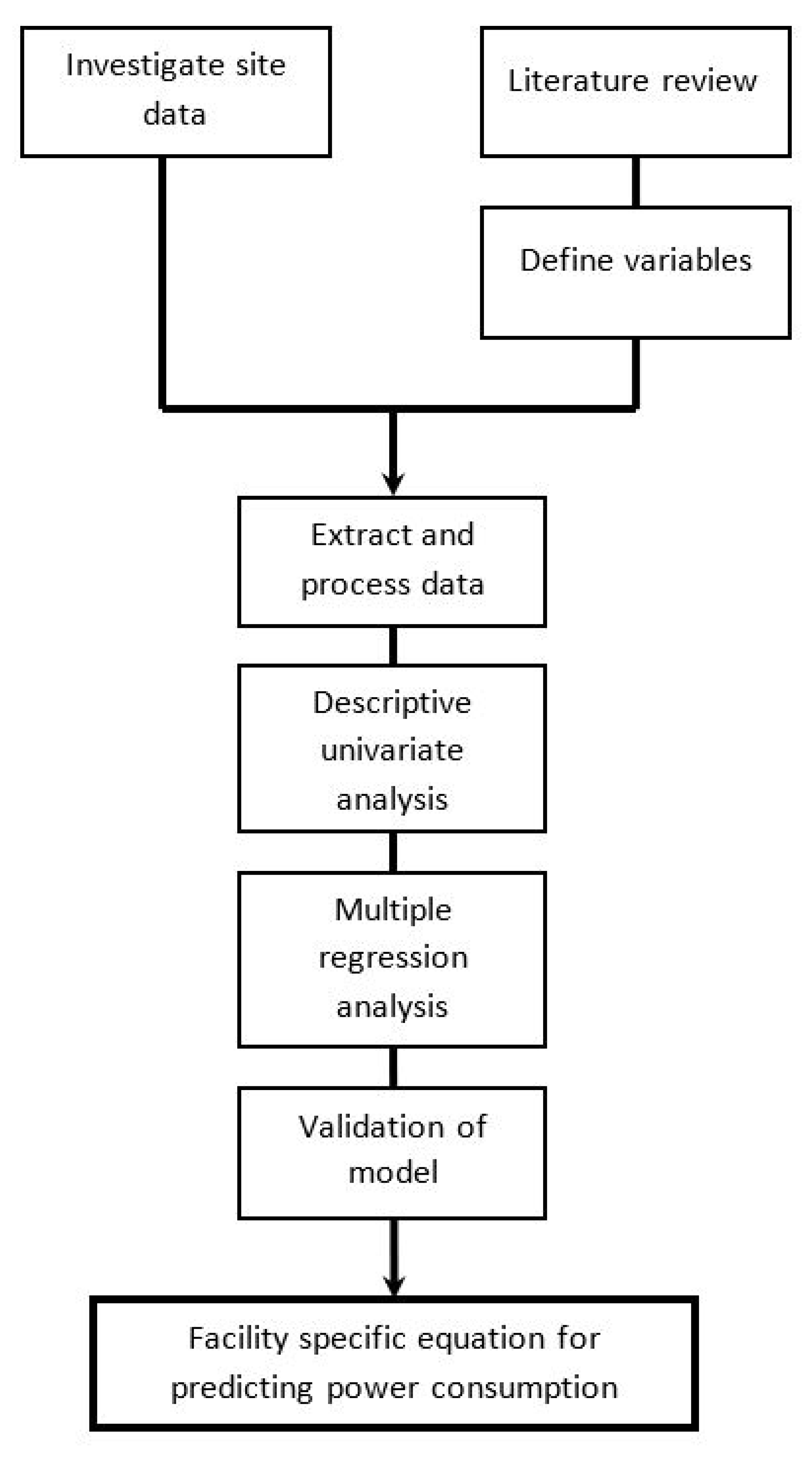
This study investigates the impact of several independent variables on the energy use of a swimming facility. The analysis has been carried out by applying the multiple linear regression method with the purpose of developing a reliable energy prediction model. Figure 2 illustrates the workflow of the study, where the main topics are identified.

2.1. The Building

The investigated building is a multi¬purpose sports center located at Jøa, an island in the municipality of Namsos in Norway. It is located at 64.6 N, 11.2 E, 65 m above mean average sea level. It is defined as part of the Marine West Coast climate zone according to the climate zone definition of Köppen and Geiger [42]. The sport center was commissioned in autumn 2016 and contains several facilities besides the swimming pool facility, such as a sports hall, a shooting range, a library, a café, a gym and an outdoor ice rink. Figure 3 shows a photograph of the north-oriented façade for the swimming hall. The swimming hall has a usable area of 266 m² (13.7 m × 9.43 m), including the 8.5 m × 12.5 m swimming pool. Key quantities are presented in Appendix B. This paper investigates only the part of the building with the swimming facilities.

2.2. The Technical Systems

The swimming facility at Jøa is a state-of-the-art swimming facility which complies with the Norwegian passive house standard [22]. It includes a ventilation heat recovery system equipped with a heat pump, as recommended in the literature [5,43], and conventional water treatment, which research has found to be the most effective water treatment train [44].

2.3. The Dataset

The dataset ranges from November 2017 to June 2019 and is separated into two parts. The training dataset and the validation dataset are, respectively, from November 2017 to June 2018 and September 2018 to June 2019. The size of the datasets was decided based on three main factors: (1) The training dataset should not be too large, due to the purpose of the study; it should be a quick and easy to implement a dynamic energy benchmark for swimming facilities. (2) The validation dataset should be large enough to cover all the seasons and several operation disruptions. (3) It should be preferably based on continuous operation data, without including lockdowns for maintenance.

2.4. The Variables

The objective of the study is to predict the energy use (dependent variable) as a result of several independent variables. The selected independent variables used in this study are listed in Table 1.
The dependent variable was defined by applying the energy conservation Equation (1) at the boundary defining the swimming facility as presented in Figure 1.
d E n e t d t = E ˙ n e t = E ˙ e a + E ˙ t a + E ˙ e p + E ˙ t p
where Ėnet is the net delivered energy to the facility, Ėea is the delivered electricity to the air handling unit, Ėta is the delivered thermal energy to the air handling unit, Ėep is the delivered electricity to the pool circuit and Ėtp is the delivered thermal energy to the pool circuit. The units for the variables are given in Table 1.
The independent variables were defined as the meteorological data, ambient air temperature and relative humidity and the usage data. This choice was due to the availability in the respective building and to the known correlation between energy use and outdoor climate [45] and user interference [7,36,45]. In addition, this group of indicators is represented as logged values in conventional building automation systems (BASs). Due to the highly insulated building envelope and the orientation of the façades, the assumption of negligible effects of wind pressure and solar radiation was applied.
The dataset was created by:
1
Extracting historic data from the BAS.
2
Collecting weather data from the national database of the Norwegian Meteorological Institute [46].
3
Digitalizing handwritten occupancy data due to lack of electronic occupancy registration.
4
Calculating new variables based on indirectly monitored data. This is reported for the respective variables in Table 1.
Due to implications within the BAS, extracting data prior November 2017 was not possible. In addition, only a limited part of the variables was logged in June 2018. Table 1 summarizes the variables in the dataset, the units and the origin of the data.

Cleaning the Dataset

The resolution of the original training dataset was 1 min time steps for all the variables. The dataset was cleaned and preprocessed by detecting and analyzing outliers manually, caused by broken sensors, miscoded values, operation disruption (e.g., unintended operation due to mechanical flaws, software errors or mistakes by the operator), etc. Outlier detection can also be carried out statistically, for example, by using approaches such as standard deviation or the interquartile range [47]. Both techniques identify outliers by comparing each value/measurement to its population. Due to the purpose of this study, outliers are of special interest (fault detection). For the training dataset, operation disruptions were identified and excluded prior to regression analysis, while operation disruption was a part of the validation process.
The process of identifying and categorizing operation disruptions was carried out by an in-depth investigation of the historic data, stored in the BAS and in the dedicated control systems of the air handling unit and heat recovery system.

2.5. Statistical Methodology

The choice of the multiple linear regression method was based on its strength as a statistical data handling tool and its simplicity in development, implementation and operation. The latter is crucial if the building owners and the industry are to be able to minimize the energy use, related to undesired operation, over a short period of time. Regarding practical issues, the developers (the engineers) recognize the method in their university education and the operation management can easily evaluate the energy performance in a spreadsheet [41], or it can be easily implemented in any report system, due to its simple algebraic equation.
The dataset was imported and analyzed with IBM SPSS statistical software [48].

2.5.1. Multiple Linear Regression

The MLR method was used to predict the dependent variable y, here the total power consumption, averaged over a certain period. This period was taken to be sufficiently long so that the method only focused on physical effects as processes in the steady state for each time step. The regression equation was trained by the ordinary least square method where the sum of the root square error was minimized. The corresponding regression coefficients, β 0 and β i , were determined. These comprised the slope coefficient for the independent variables.
y i = β 0 + β 1 x 1 + β 2 x 2 + + ϵ
where y i is the dependent variable, β 0 is the intersection with the y-axis when x is zero, β i is the regression slope coefficient in the linear equation, x i is the predictor—the independent variable—and ϵ is the error term.

2.5.2. Assumptions

In the development of the model, several assumptions were adopted. The data source was time series data, and, initially, its autoregressive properties or the order of the autoregressive process were not known. These were identified by applying the partial autocorrelation function (PACF), which specifies the number of past lags influencing the dependent variable (i.e., the order of the autoregressive process). The application of the PACF in time series analysis is analogous to deciding the number of independent variables to be included in a multiple linear regression analysis [49]. The dataset was initially investigated for autoregressive properties and reduced by averaging the data and centered in time to eliminate any autoregressive properties in the dependent variable. Each observation in the training dataset was then treated as independent.

2.5.3. Evaluation of the Prediction Model

The “goodness of fit” was evaluated by the coefficient of determination R 2 and the adjusted R 2 , which considers the number of explanatory variables and the possibilities of overfitting. R 2 is defined by the relationship between the explained sum of squares and the total sum of squares.
The multiple linear regression equation was validated by analyzing the variance with the F-test. The test operator, F, which is defined by the ratio between the explained sum of squares and the residual sum of squares, was applied to the F-distribution. A significance level of 5% was chosen as the required level.
The coefficients in the equation, the impacts of the independent variables, were evaluated by applying the T-statistic, with the t-test, which is similar to the F-test, but which describes the probability of nonlinear correlation by applying the test operator to the T-distribution. The test operator is defined by the relation between the coefficient and its standard error.
The fundamental assumptions for using linear regression were investigated, such as a lack of multicollinearity, no heteroskedasticity, normally distributed residuals and no autocorrelation among the residuals [50], which were fulfilled for each case in the presented analysis. The multicollinearity among the variables was investigated by manually applying the independent variables in a correlation matrix. Potential heteroskedasticity was evaluated visually. The autocorrelation among the residuals was tested with the Durbin–Watson statistic, which assumes a maximum lag of one. The lag of the residuals was investigated by determining the autoregressive process by applying the PACF.

2.5.4. Validation

The prediction model was tested and validated by comparing the prediction and measurement for the whole validation dataset. The criteria for a passed validation process were defined as (1) all the measurements identified as normal operation should be predicted within the prediction interval defined in the training process and (2) all of the operation disruptions should be clearly identified by the validation process.

3. Results and Discussion

3.1. Description—The Training Dataset

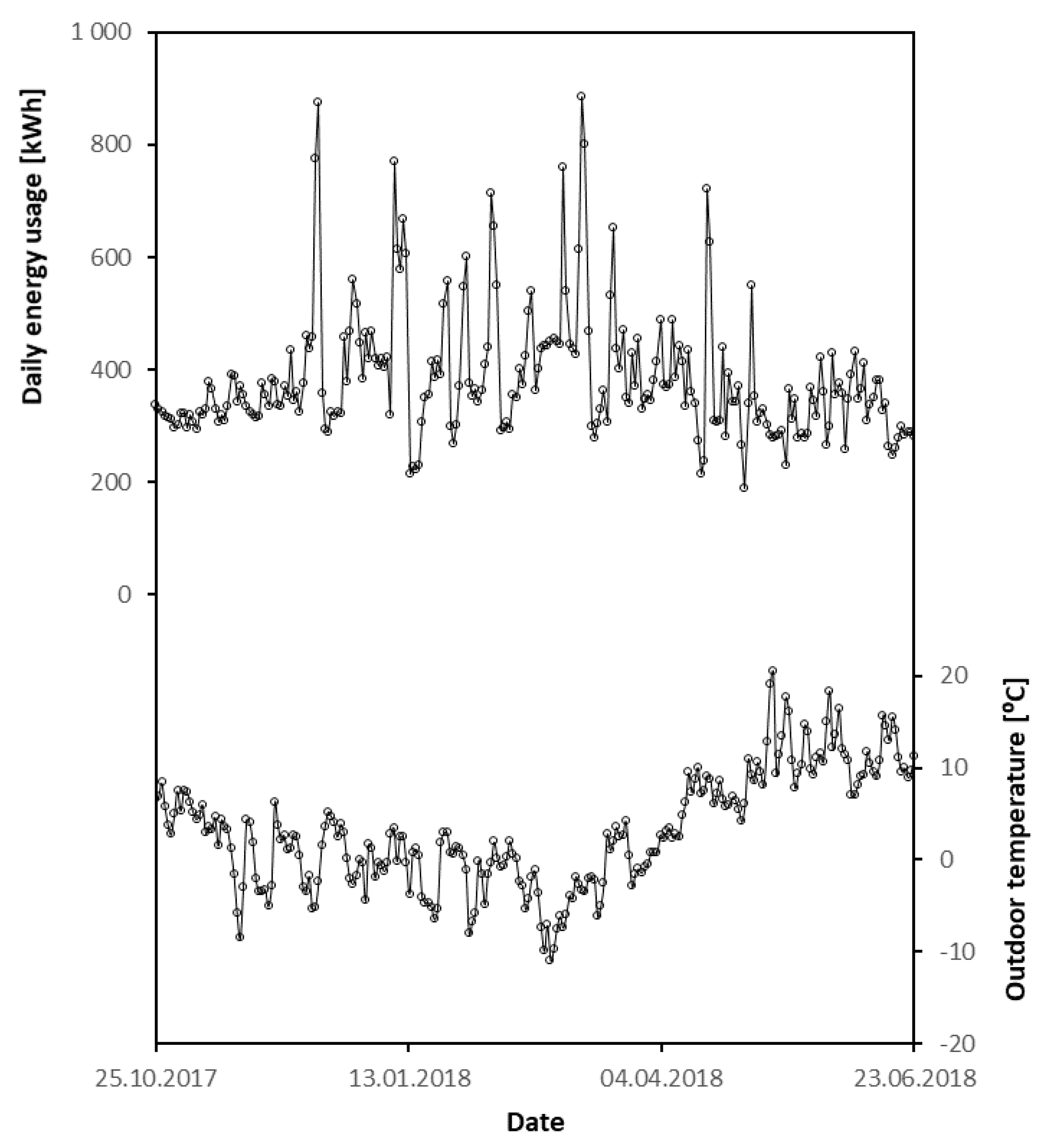
The dataset used for training the regression analysis comprises approximately 350,000 observations. Figure 4 shows the collected data for the dependent variable and the total electric and thermal power consumption, plotted together with the outdoor dry-bulb temperature. The average power consumption for the whole dataset is approximately 16 kW and energy supply for the period is 93,000 kWh. The daily average energy use ranges from approximately 190 kWh to nearly 900 kWh, with a corresponding daily average power consumption ranging from approximately 7.9 kW to 37 kW. The registered average diurnal dry-bulb temperature ranges from −11 C to 20 C. During this period, nearly 2000 swimmers used the facility, equally divided between adults and youngsters/children.
Figure 4 reveals a seasonal trend, a minor dependency between the energy use and the outdoor temperature, with some spikes in energy use distributed over the period. By visual inspection, it seems that the outdoor temperature variable can explain some of the variations in energy use, but additional variables influenced the variation in daily total energy usage.

3.1.1. The Energy Performance of the Facility

Regarding the energy performance, the swimming facility at Jøa was identified as having an energy performance indicator (EPI) of 44.8 kWh/visitor, calculated over the period of the investigated dataset presented in Figure 4. In comparison, Norwegian swimming facilities are associated with an average EPI for a typical year of approximately 26 kWh/visitor, and a median EPI of approximately 22 kWh/visitor, where the dispersion is reported to range from 10 to 80 kWh/visitor [51]. The EPI has been recommended by Kampel [7] who found that visitors are the single variable that explains most of the variation in the energy performance of swimming facilities [35]. The poor EPI-value of the swimming facility at Jøa can be explained by the low user intensity, on average only 235 visitor/month, compared to Kampel’s dataset representing a median annual user intensity of 94,261 visitors (average of 7855 visitors per month). Additionally, the outdoor climate can explain this performance indicator since the data are not climate corrected.

3.1.2. Energy Distribution

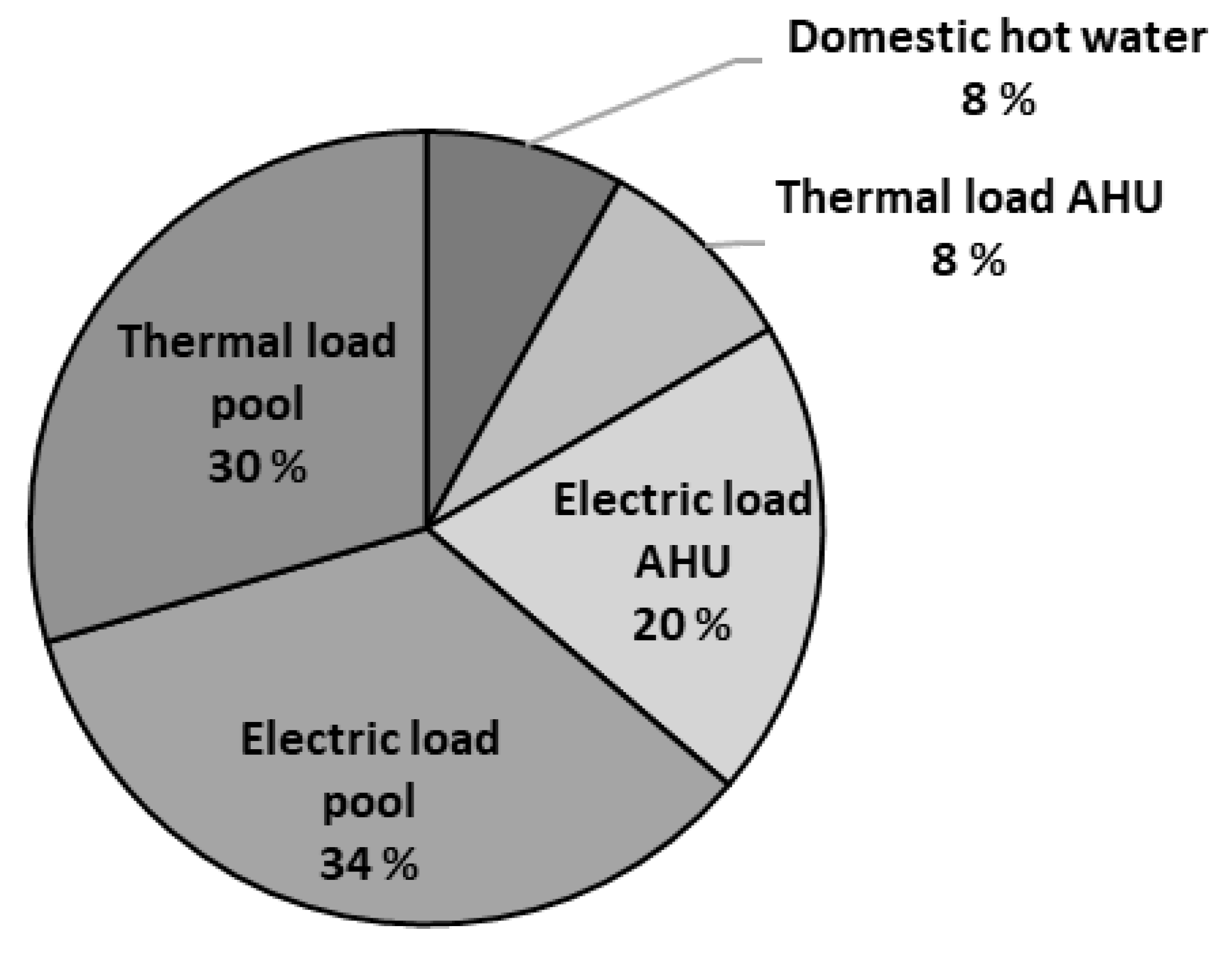
The delivered energy to the swimming facility is almost evenly divided between electricity and thermal energy. Figure 5 depicts the energy distribution of the building section with the swimming pool. The low thermal energy consumption for the air handling unit (AHU) in comparison with the thermal load of the pool circuit has two major causes. The low overall user intensity for the period of collected data implies that the system operates in air recycling mode (night mode) without fresh air supply for a long period of time, which reduces the air dehumidification and heating demands considerably. Another reason is the operation of the heat recovery system which recovers the latent heat in the exhaust air and supplies heat to the facility, where the order of priority is air heating and pool heating. The building automation system neither collects data regarding the performance of the subsystems nor the thermal efficiency of the heat recovery system.

3.1.3. Time Step Analysis

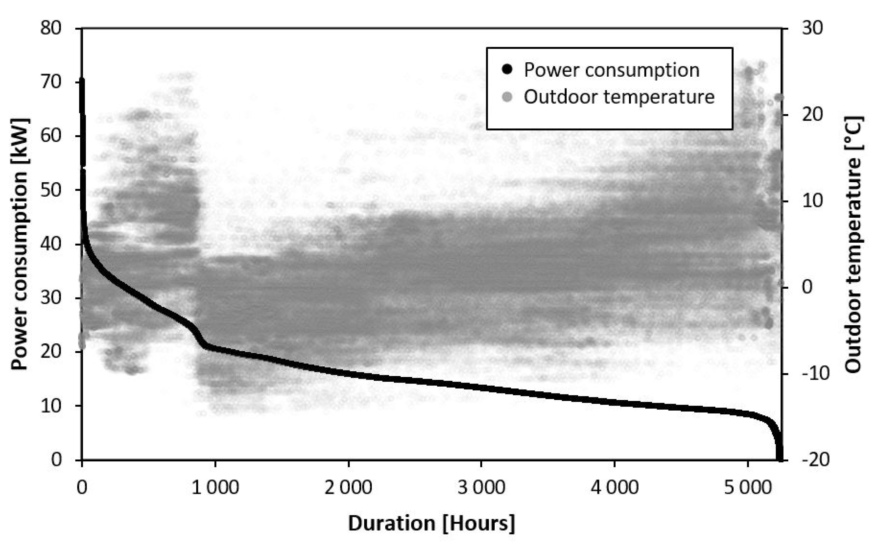
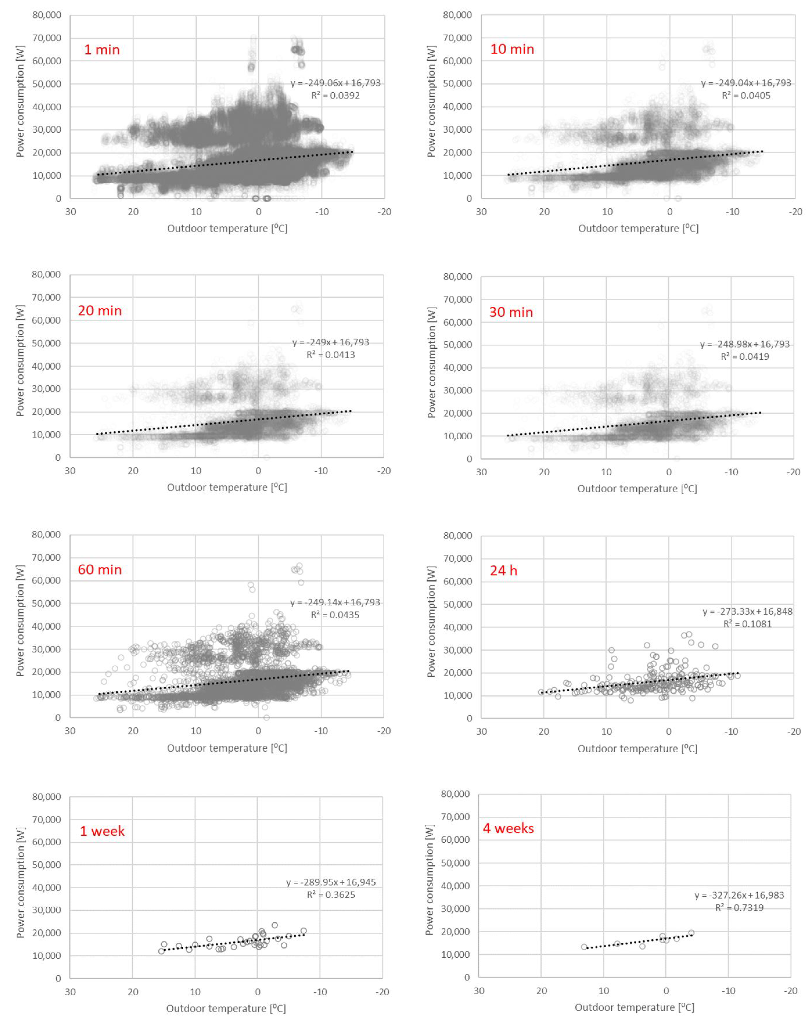
When treating time series data of energy use in buildings with linear regression, the inertia of the building must be considered due to this impact on the autoregressive process of the variables. This is because the energy use (the dependent variable) is logged with a short time step (1 min). For the swimming pool at Jøa, this impact is partly illustrated using a duration curve depicted in Figure 6, where the data are sorted by decreasing power consumption. The range of outdoor temperatures associated with each step of power demand is wide and can be partly explained by inertia of the building. A short time step resolution will not give any significant correlation, since the process depicted is not steady state. The impact of the time lag can be minimized by averaging the dataset, and thereby reducing the time step resolution (see Section 2.5.2).
Figure 7 illustrates the consequences of averaging the dataset and reducing the time step resolution. The figure presents the dataset with time steps ranging from 1 min to 4 weeks. Both the power consumption and outdoor temperature are presented as time-averaged values centered in time. Firstly, the figure gives an indication of two possible different states in the operation of the facility, represented as a pattern of a divided dataset (clouds of datapoints), for time-step resolution from 1 min up to 60 min. The same can be observed in Figure 6, which represents a pattern of two different duration curves overlapping. Secondly, without considering the significance of the simple linear regressions, a considerable increase in the coefficient of determination, the R 2 , is observed when averaging the dataset. This implies that the time step should be maximized in order to obtain the best fitting model if prediction is the main purpose. Concerning the purpose of this study, the time step should correspond to the swimming facility operating staff’s requirement to identify and handle possible operational disturbances during a reasonable period of time.

3.2. Statistical Analysis—Developing the Model

Since the training dataset consists of operation data from the first period after the building was commissioned, several irregularities may occur. By detecting and excluding observations associated with irregular operation events, the training dataset is optimized to only represent flawless operation. A predictive model trained by this dataset should be able to provide accurate predictions.
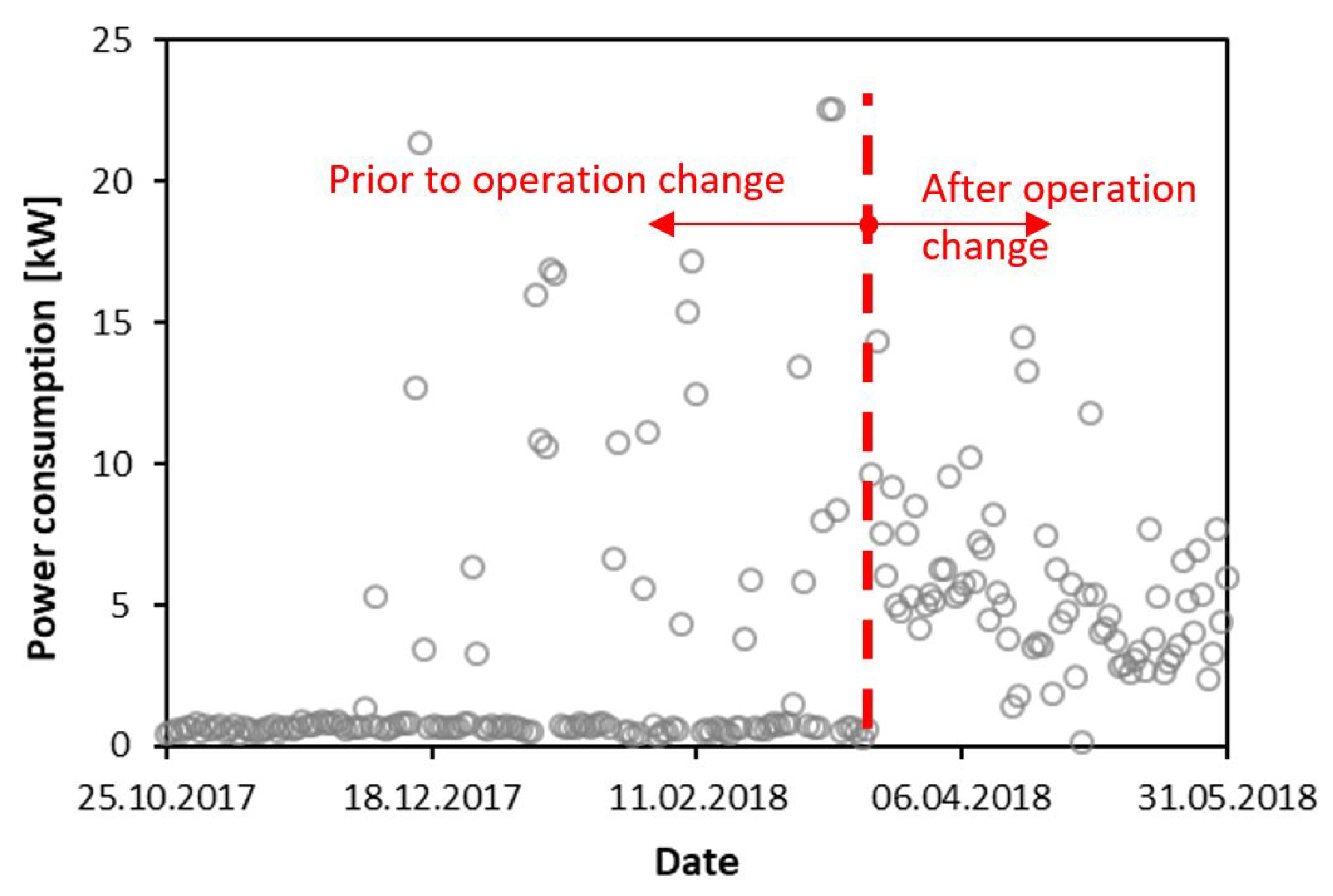
By investigating historical operating data from both the BAS and the internal control system of the air handling unit, a major change in operation was found. The consequence of this is illustrated in Figure 8, which depicts the thermal load for the pool heating system, where a change in operation is identified in late March 2018. The reason for the considerable change was issues related to the control of the integrated dehumidification system and the pool temperature, possibly a problem with a mixing valve. However, since this flaw in the operation has implications for both the pool temperature and the heat recovery system, the whole period from 25 October 2017–22 March 2018 must be excluded from the training dataset.

New Training Dataset

By excluding the period associated with operational irregularities, prior to 22 March 2018, the prediction model was developed. The new training dataset, ranging from 22 March to 24 June 2018, consisted of three-day averaged values, for a total of 29 datapoints. The analysis of the autoregressive properties of the dataset showed no autocorrelation when averaging data for 72 h, or 3 days.
The results of the regression analysis are expressed in Equation (3). The key output from the regression analysis is given in Table 2. Regarding possible problems with overfitting, 15 datapoints per predictor are recommended [52] to obtain reliable fitted regression, which means a maximum of two predictors for a dataset of this size. The two independent variables which are found to explain most of the variance are the outdoor dry-bulb temperature ( T o u t ) and the pool usage factor ( t p u ) (see description of variables in Table 1). This combination has a statistical effect on the energy use, with almost similar impact, and both were identified by a significance level p < 5%. The chosen combination of variables is in accordance with the physics, where the outdoor temperature represents the thermal losses through the envelope and ventilation, and the pool usage represents the water usage and the operation mode of the facility. The number of swimmers was not found to have a statistical effect on the overall power consumption, despite the impact of evaporation on the energy use. This may be explained by the phenomenon of evaporation, which is observed as a step function where a few bathers have a significant impact, but a further increase only gives a small additional contribution to evaporation [53]. However, the combination of weather conditions and usage/occupancy is also found to have a statistically significant effect on energy use in office buildings [38], despite the difference between these building categories.
E ˙ t o t = 14 , 715 227.8 T o u t + 24 , 790 t p u
where Ėtot is the predicted power consumption [Watt], T o u t is the outdoor temperature [°C] and t p u is the pool usage factor.
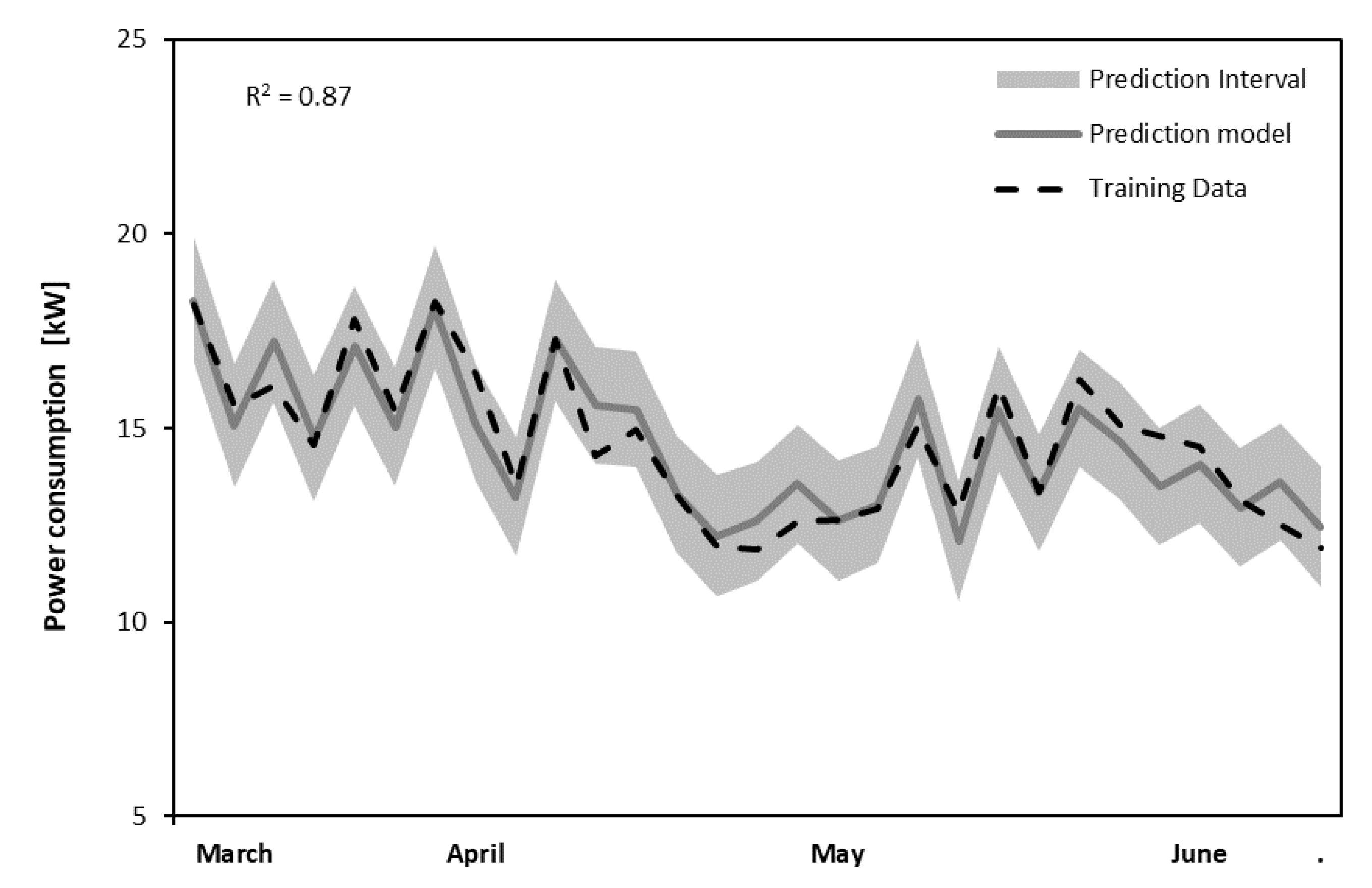
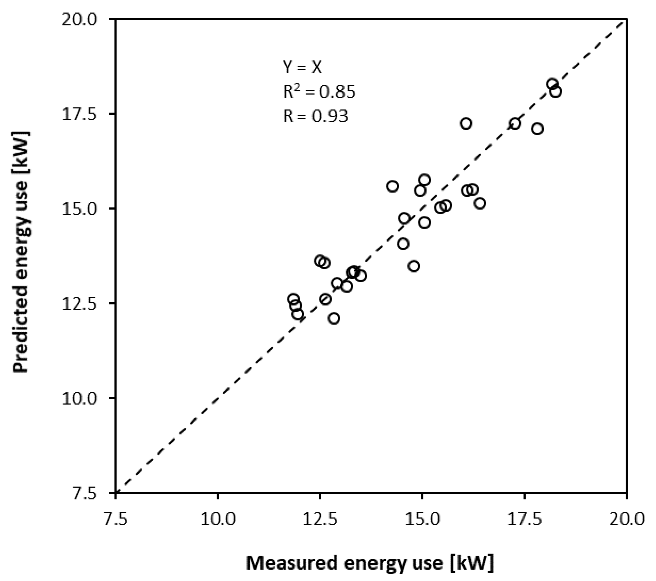
The ability of the model to explain the variance is given by R 2 = 87%. The ability of the prediction model to reproduce the power consumption is illustrated in Figure 9, where the predicted power consumption is plotted along with the training data, the actual power consumption and the corresponding prediction interval. The prediction interval of 95% is the interval where there is 95% confidence of there being an observation within it. It depends on factors like sample size, number of predictors and the significance level. For the range of independent variables given in the training dataset, the mean prediction interval is identified to be ±1.86 kW. Figure 10 shows the linear relationship between the training dataset and the data produced by the prediction model where the Pearson correlation coefficient is 0.93.
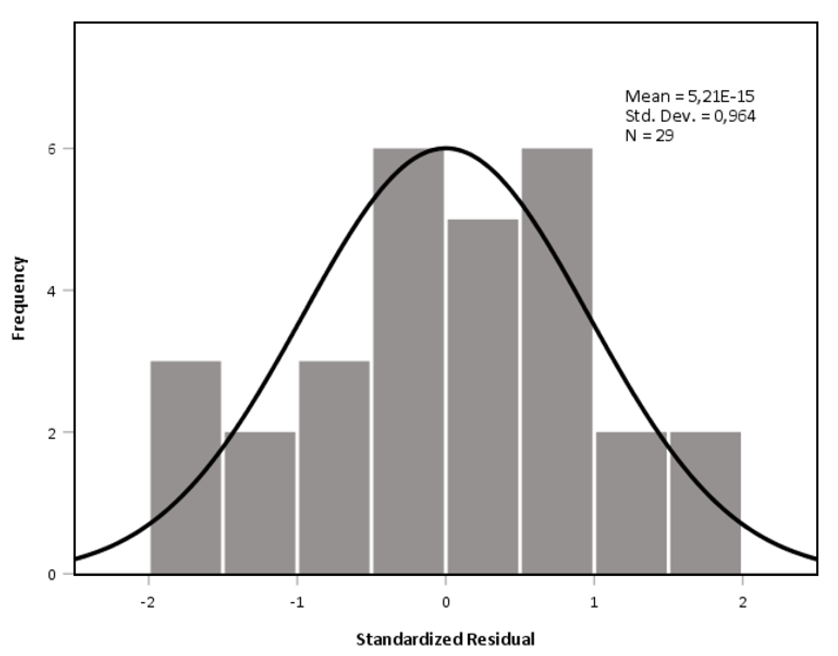
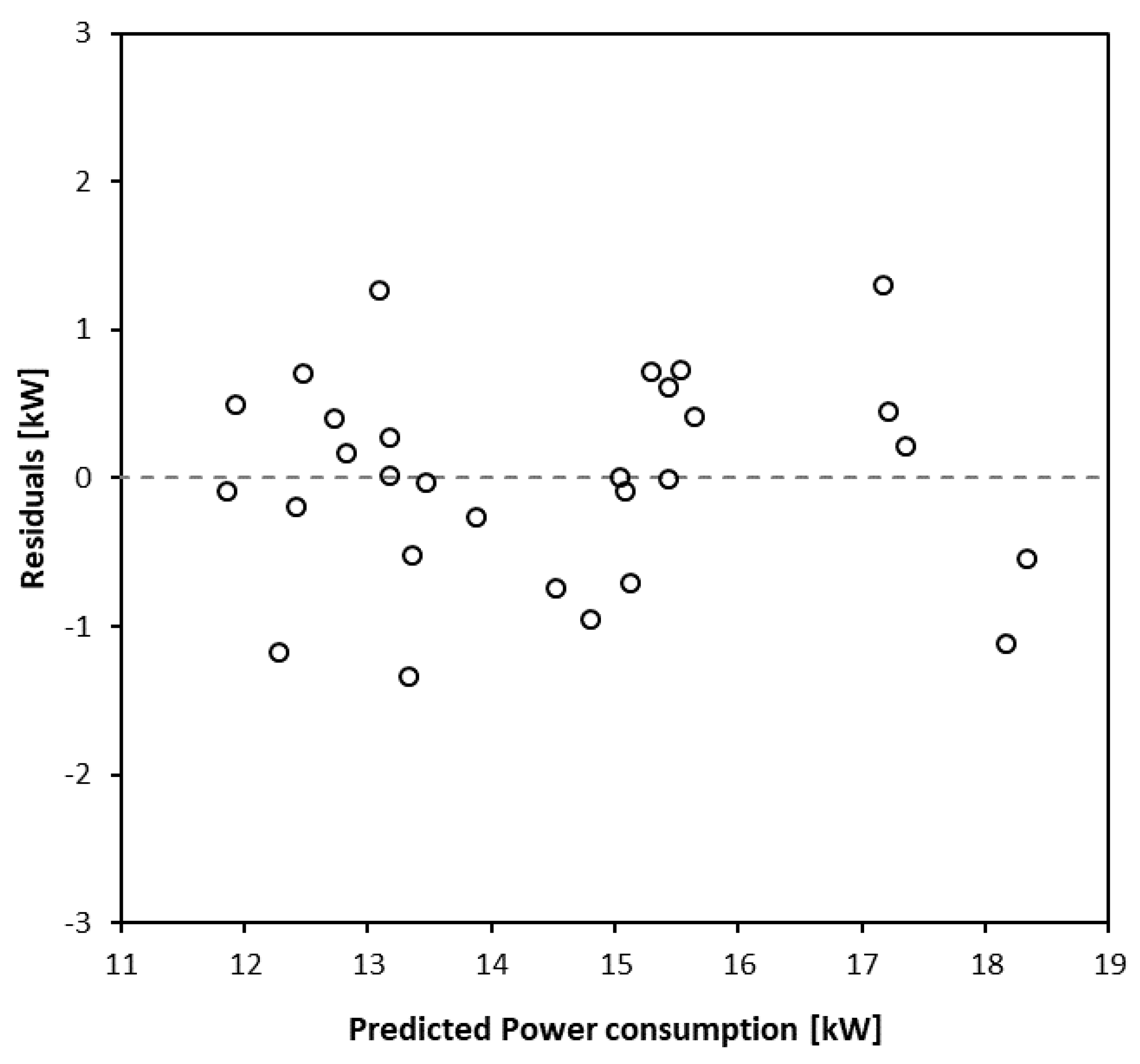
Regarding the fundamental assumptions in linear regression, the residuals from the training process, given in Figure 11 and Figure 12, are approximately normally distributed. There are no signs of heteroskedasticity and the residuals are represented with a mean value of approximately 0. The autoregressive process is not found to be on an order higher than 1, but the Durbin–Watson coefficient is approximately 1.4, which possibly indicates some autocorrelation. However, the possible autocorrelation, or the lack of autocorrelation, is not found to be statistically significant. The regression equation is considered to be reliable within the given goodness of fit.

3.3. Validation and Application

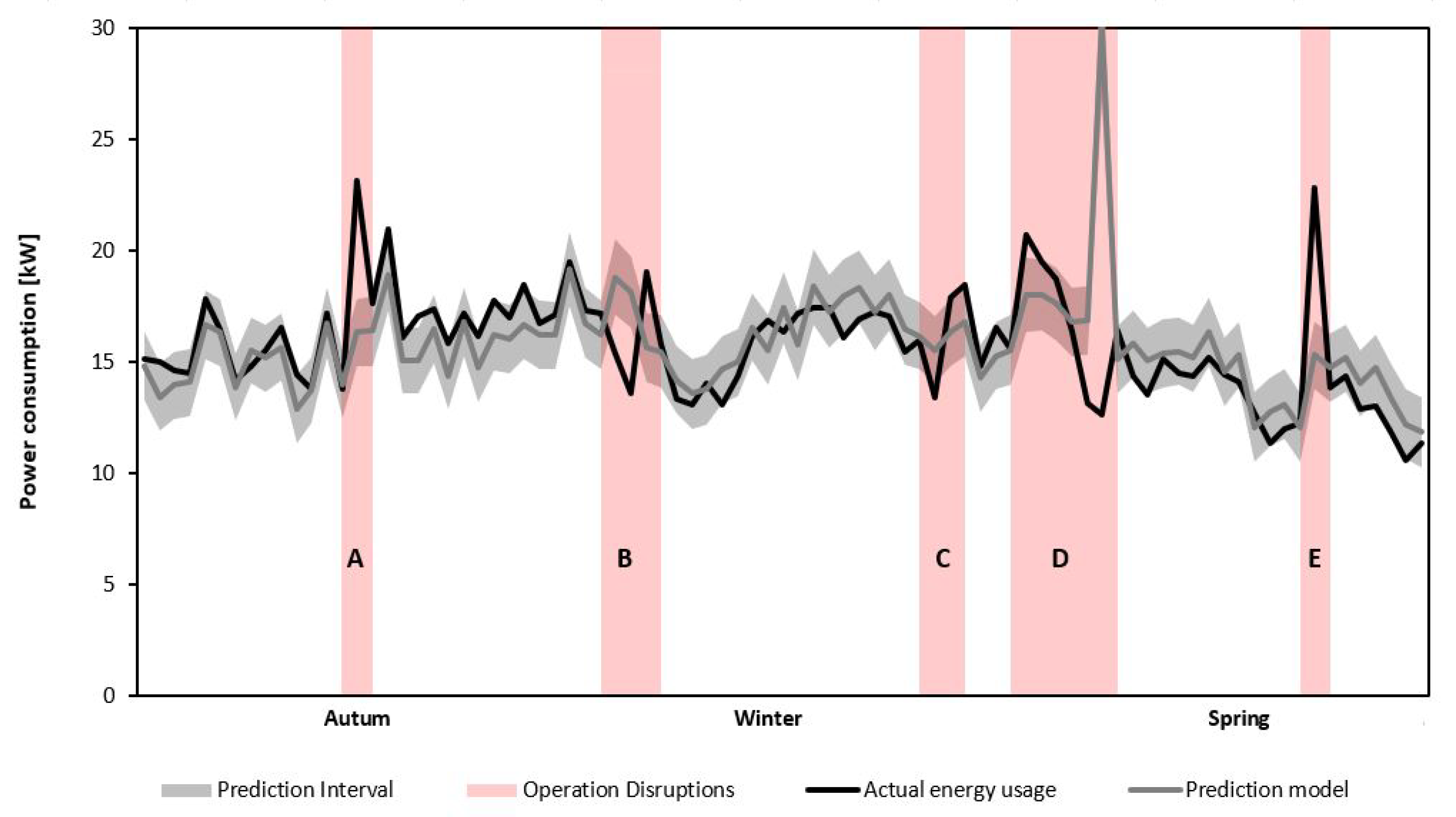
The validation of the prediction model is illustrated in Figure 13 as a comparison between the predicted and actual data from the validation dataset. The predicted power consumption, including the prediction interval, is the gray shaded area and the measured power consumption is the black line. The numbered red areas are the identified periods with operational disruption, and they include 14 datapoints out of a total of 85 in the validation dataset. The given operation disruptions have been identified as (A) uncontrolled water refill, (B,C) issues with the control system of the water temperature, (D) issues with controlling the indoor environment and water refill system, leading to a consecutive lockdown of the facility and (E) issues related to the control of the air handling unit and the air flow supply. The prediction model identifies all of the disruptions as illustrated. When the facility operates without flaws and faults, the facility performs within the operational baseline provided by the prediction model. Each of the operational disruptions are identified as major deviations from the baseline.
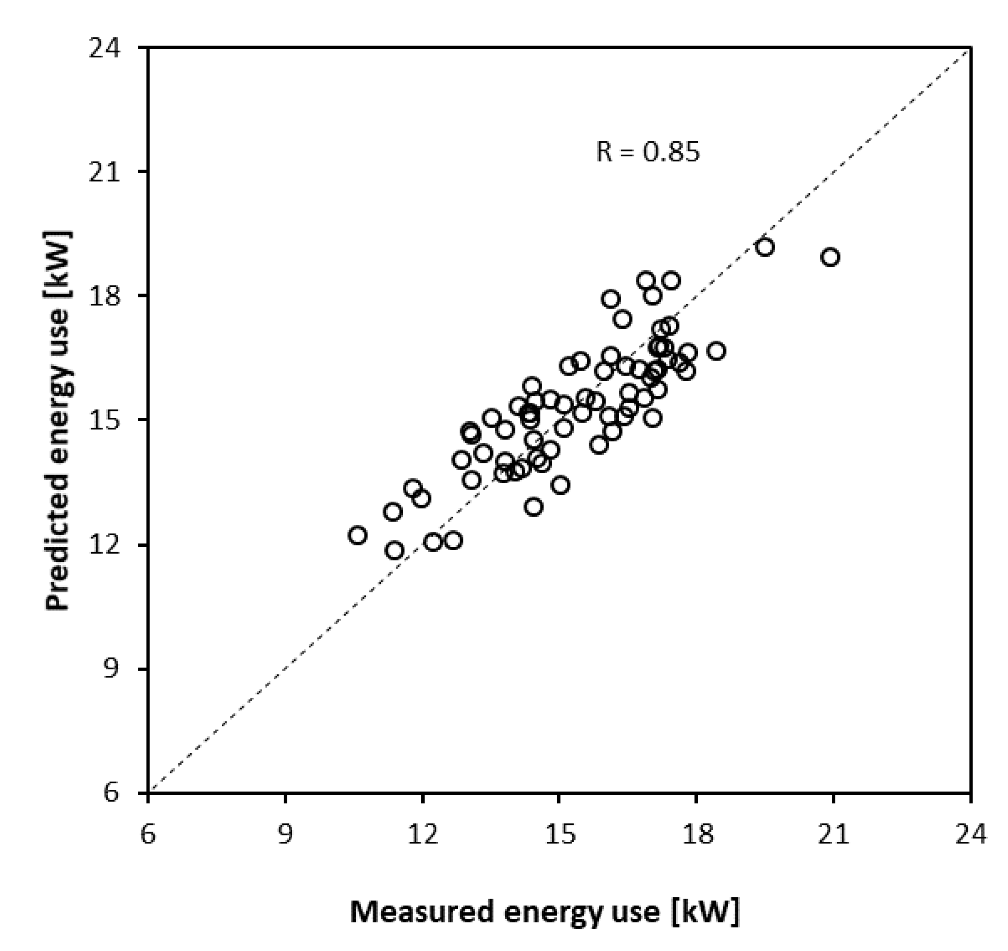
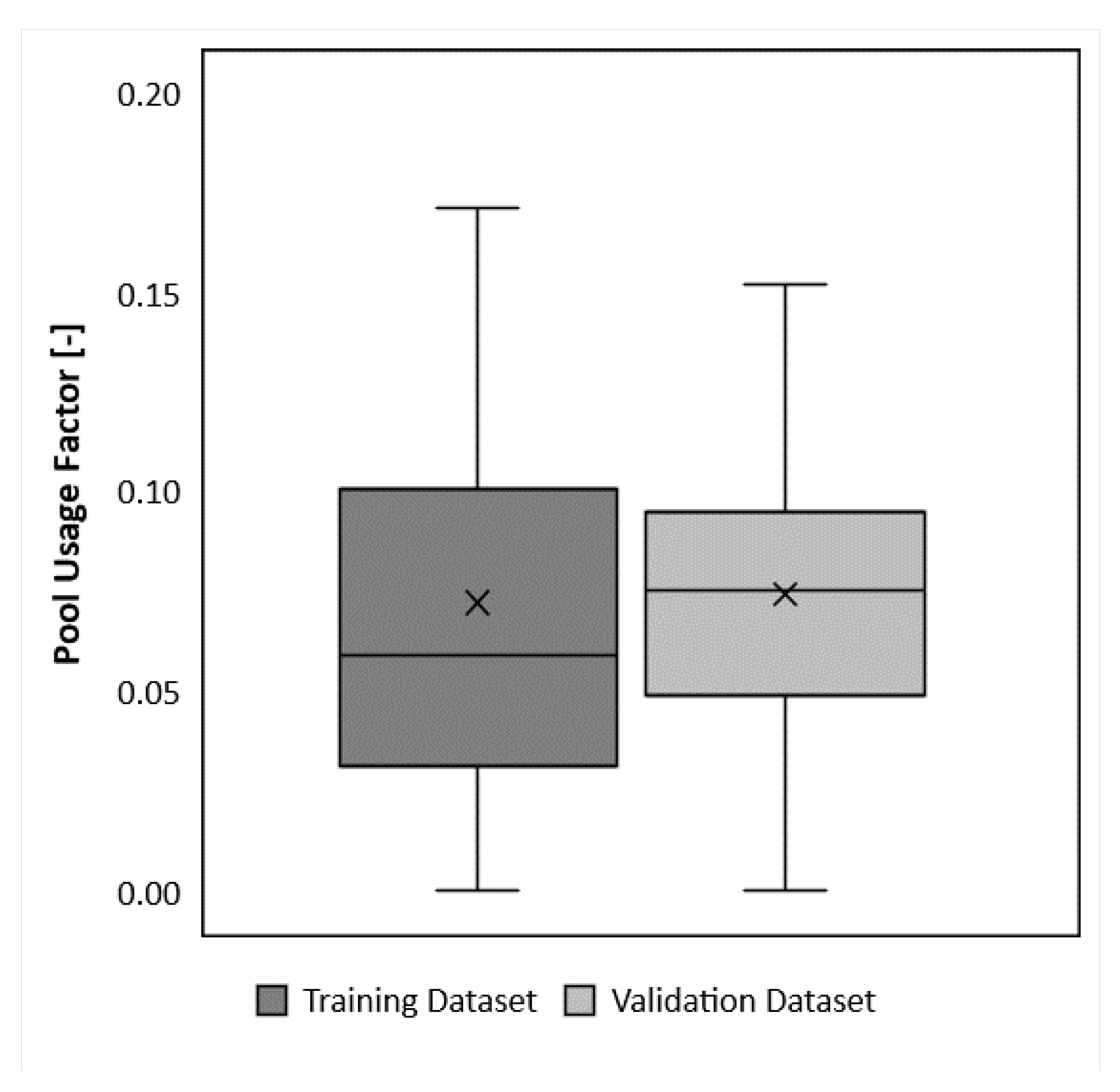
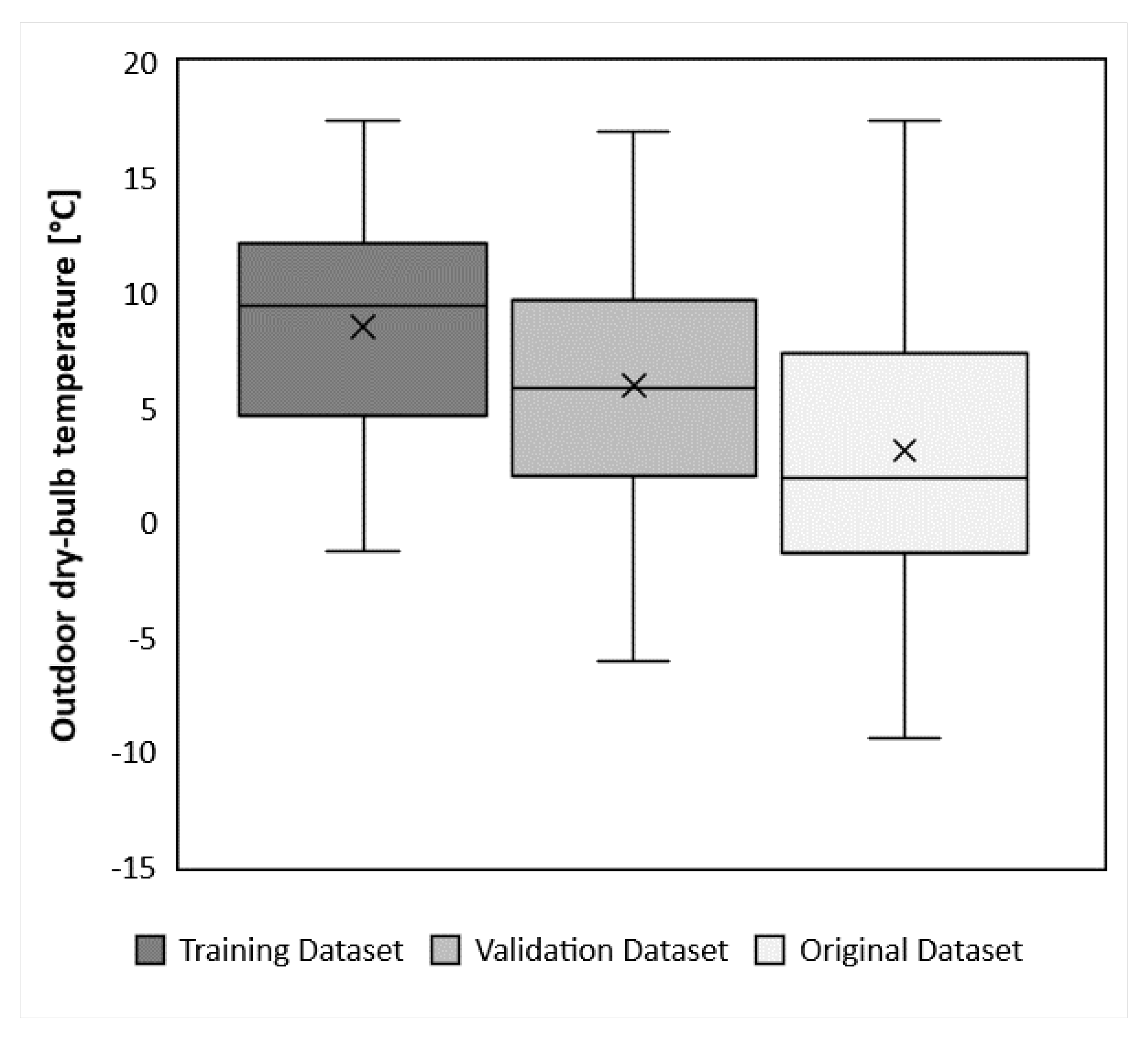
When excluding the data associated with operational disruptions, 14 datapoints in total (approximately 16% of the dataset), the predicted operation fits the actual performance well. Figure 14 illustrates the correlation between the predicted and measured power consumption exclusive of the operation disruptions. The Pearson correlation coefficient is 0.85. However, there are periods where the models seem to consistently over- or underpredict the performance model, and this may have to do with the lack of explanatory variables in the model. However, this deviation is within the prediction interval, which corresponds with no detection of operational disruption for the relevant period. Figure 15 and Figure 16 present the range of the independent variables used in the prediction model. Even though the range of the training dataset was initially significantly reduced to only three months of data (29 datapoints), the dispersion of the variables within this dataset corresponds with the validation dataset.
In the perspective of applying the presented method to industry, the combination of a short-term training dataset and the few predictors makes this method especially useful. This means that a facility can develop a model over a short period of time, with a minimum of sensors. However, the transferability with regard to the choice of independent variables must be further investigated in order to obtain a universal method for industry.

4. Discussion and Opportunities for Deployment of the Created Model

Due to the importance of focusing on the operating phase when minimizing the environmental impact [10,54], and because operational irregularities are common in buildings [55], an implemented operational tool may have great potential for industry. For swimming facilities, this is especially important since inappropriate operation may also cause problems such as degradation of equipment and the occurrence of the sick building syndrome [56]. When applying the presented method to industry, the combination of a short-term training dataset and a few predictors makes this method especially useful. It means that a facility can develop a personalized model in short period of time with a minimum of sensors. In addition, the final energy prediction model is simple and can be deployed either in a spreadsheet or in the building automation reporting system. This method can therefore contribute instantly to keep the operation of a swimming facility within the optimal and expected individual energy performance range, which is fundamental for achieving the energy target for any building [57]. The MLR method, which is applied in this study, has formerly been recognized for predicting energy use in buildings [39] and has also been applied to determine the parameters of thermal equations for outdoor swimming pools [58]. With respect to the specific case of Jøa, the operational staff have to download the energy usage, the outdoor temperature and the pool usage. The deviation between the prediction and the measured energy use will give the operational staff an alarm if there is a potential flaw in the operation and enable them to detect the fault within a short period of time. However, the transferability with respect to the choice of independent variables must be further investigated in order to obtain a universal method for industry. Additionally, guidelines with respect to the implementation of the model should be provided.

5. Conclusions

This paper presents a model for predicting energy consumption in swimming facilities. The energy prediction model aims to become a dynamic energy benchmark for fault detection in swimming facilities. The investigation has been carried out by using multiple linear regression analysis (MLR) for a specific swimming facility located in Norway. The MLR method has formerly been recognized in predicting energy use in buildings but has also been applied to determine the parameters of thermal equations for outdoor swimming pools. The main findings of this study are:
  • The study has shown that it is possible to develop an accurate energy prediction model for swimming facilities with a minimum of variables and datapoints.
  • The results from the analysis of the training dataset underlined the importance of investigating the training data prior to training of the model. The original dataset was based on raw data from 7 months of operation after the building was commissioned and approved by the building owner. The modified and preferred dataset was reduced after an in-depth investigation that revealed comprehensive operational disruptions. The final training dataset consisted of only 29 datapoints of 3-day averaged data ranging over a period of 3 months, March to June 2018.
  • The statistically significant independent variables were found to be the outdoor dry-bulb temperature and the pool usage factor, which predicted the average power consumption accurately in the validation process. In the validation period from September 2018 to June 2019, the equation correctly identified all the critical operational disruptions.
  • The model has been shown to be a suitable tool for helping operating staff in continuous evaluation of the energy performance of a facility and quickly disclosing possible operational disruptions. By identifying possible operational irregularities at an early stage, excessive energy use in operation can be avoided. Operational irregularities occur in a high percentage of new buildings. The importance of focusing on the operating phase and the overall energy consumption is crucial when minimizing the environmental impact. In addition, the knowledge of the energy performance of buildings is fundamental in achieving the energy targets. For swimming facilities, inappropriate operation of technical installations may also cause problems such as degradation of equipment and the occurrence of sick building syndrome.
  • This study only investigated one specific facility and future work should address the robustness of the model and transferability to other swimming facilities.
This study illustrates the strength of multiple regression analysis when applied as a dynamic and continuous energy benchmark. By applying simple input variables, an estimate of the expected power consumption, within an acceptable error range, can be made that reveals potential operational disruptions. The energy prediction model is simple and can be easily implemented in the automation system of a building. The prediction model does not require an operator with an engineering background and may serve as first-line supervision for the use of a dynamic energy benchmark for a facility. By applying this method in existing swimming facilities, the overall energy use may be greatly reduced as it provides the building management with improved knowledge about the energy performance of the building.

Author Contributions

Conceptualization, O.Ø.S.; methodology, O.Ø.S. and T.J.; software, O.Ø.S.; validation, O.Ø.S.; formal analysis, O.Ø.S.; investigation, O.Ø.S.; data curation, O.Ø.S.; writing—original draft preparation, O.Ø.S.; writing—review and editing, O.Ø.S., T.J., B.A., J.S., L.G. and S.C.; visualization, O.Ø.S.; supervision, T.J., B.A., L.G. and S.C.; project administration, O.Ø.S. and J.S. All authors have read and agreed to the published version of the manuscript.

Funding

The project is funded by COWI AS, the Research Council of Norway and COWIFonden.

Institutional Review Board Statement

Not applicable.

Informed Consent Statement

Not applicable.

Data Availability Statement

This data collection campaign was performed within the framework of a PhD study by COWI AS and NTNU SIAT. All the data are privately stored and will not be disclosed until the end of the study.

Acknowledgments

This work is a part of a doctoral project entitled “Optimizing Energy and Climate Systems in Buildings with Swimming Facilities”, which is carried out as a cooperation project between the Centre for Sport Facilities and Technology at the Norwegian University of Science and Technology in Trondheim, Norway, and the engineering company COWI AS.

Conflicts of Interest

The authors declare no conflict of interest.

Appendix A

Figure A1. Visual validation of the prediction model from September 2018 to June 2019. The prediction model includes the prediction interval in gray, measured power consumption in black and periods associated with operational disruptions in red.
Energies 14 04825 g0a1

Appendix B

SubjectQuantity
Window surface area30 m 2
Water surface12.5 m × 8.5 m
Useable area266 m 2
Nominal air flow, air handling unit11,000 m 3 /h
Nominal thermal power, air condenser26 kW
Nominal thermal power, pool water condenser34 kW
Nominal water flow circulation pool circuit60 m 3 /h
Rating condition pool circuit300 visitors/day
Nominal power pool heater70 kW

References

  1. Progress Made in Cutting Emissions. 2020. Available online: https://ec.europa.eu/clima/policies/strategies/progress_en (accessed on 15 April 2021).
  2. The European Green Deal. Available online: https://eur-lex.europa.eu/resource.html?uri=cellar:b828d165-1c22-11ea-8c1f-01aa75ed71a1.0002.02/DOC_1&format=PDF (accessed on 1 August 2021).
  3. Energy Roadmap 2050. Available online: https://eur-lex.europa.eu/LexUriServ/LexUriServ.do?uri=COM:2011:0885:FIN:EN:PDF (accessed on 1 August 2021).
  4. Ratajczak, K.; Szczechowiak, E. Energy consumption decreasing strategy for indoor swimming pools–Decentralized Ventilation system with a heat pump. Energy Build. 2020, 206, 109574. [Google Scholar] [CrossRef]
  5. Ratajczak, K.; Szczechowiak, E. The Use of a Heat Pump in a Ventilation Unit as an Economical and Ecological Source of Heat for the Ventilation System of an Indoor Swimming Pool Facility. Energies 2020, 13, 6695. [Google Scholar] [CrossRef]
  6. Kampel, W.; Aas, B.; Bruland, A. Energy-use in Norwegian swimming halls. Energy Build. 2013, 59, 181–186. [Google Scholar] [CrossRef]
  7. Kampel, W. Energy Efficiency in Swimming Facilities. 2015. Available online: https://ntnuopen.ntnu.no/ntnu-xmlui/handle/11250/2366793 (accessed on 20 November 2020).
  8. Røkenes, H. Betraktninger Rundt Svømmehallers Energieffektivitet. Master’s Thesis, Norwegian University of Science and Technology, Trondheim, Norway. 2011. [Google Scholar]
  9. Swim England. The Use of Energy in Swimming Pools. 2016. Available online: https://www.swimming.org/library/documents/1187/download (accessed on 24 March 2021).
  10. Rincón, L.; Castell, A.; Pérez, G.; Solé, C.; Boer, D.; Cabeza, L.F. Evaluation of the environmental impact of experimental buildings with different constructive systems using Material Flow Analysis and Life Cycle Assessment. Appl. Energy 2013, 109, 544–552. [Google Scholar] [CrossRef]
  11. Catrini, P.; Curto, D.; Franzitta, V.; Cardona, F. Improving energy efficiency of commercial buildings by Combined Heat Cooling and Power plants. Sustain. Cities Soc. 2020, 60, 102157. [Google Scholar] [CrossRef]
  12. GlobalABC/IEA/UNEP (Global Alliance for Buildings and Construction, International Energy Agency, and the United Nations Environment Programme). GlobalABC Roadmap for Buildings and Construction: Towards a Zero-Emission, Efficient and Resilient Buildings and Construction Sector; IEA: Paris, France, 2020. [Google Scholar]
  13. ASHRAE. Applications Handbook. American Society of Heating, Refrigerating and Air-Conditioning Engineers; ASHRAE: Atlanta, GA, USA, 2015. [Google Scholar]
  14. Smedegård, O.; Aas, B.; Stene, J.; Georges, L.; Carlucci, S. A Systematic and Data-Driven Literature Review on the Energy and Environmental Performance of Swimming Facilities. Unpublished work. 2021. [Google Scholar]
  15. Djuric, N. Real-Time Supervision of Building HVAC System Performance. 2008. Available online: https://ntnuopen.ntnu.no/ntnu-xmlui/handle/11250/231184 (accessed on 24 November 2020).
  16. Nord, N.; Novakovic, V.; Frydenlund, F. Kontinuerlig Funksjonskontroll for Effektiv Drift av Bygninger; SINTEF: Oslo, Norway, 2012. [Google Scholar]
  17. Ruparathna, R.; Hewage, K.; Sadiq, R. Developing a level of service (LOS) index for operational management of public buildings. Sustain. Cities Soc. 2017, 34, 159–173. [Google Scholar] [CrossRef] [Green Version]
  18. Saleem, S.; Haider, H.; Hu, G.; Hewage, K.; Sadiq, R. Performance indicators for aquatic centres in Canada: Identification and selection using fuzzy based methods. Sci. Total Environ. 2021, 751, 141619. [Google Scholar] [CrossRef]
  19. Berardi, U. Sustainability assessment in the construction sector: Rating systems and rated buildings. Sustain. Dev. 2012, 20, 411–424. [Google Scholar] [CrossRef]
  20. The Norwegian Ministry of Petroleum and Energy. Energy Labelling Regulations for Buildings. 2010. Available online: https://lovdata.no/dokument/SF/forskrift/2009-12-18-1665 (accessed on 25 November 2020).
  21. NS 3700. Criteria for Passive Houses and Low Energy Houses: Residential Buildings (Original: Kriterier for Passivhus og Lavenergihus: Boligbyginger). 2013. Available online: https://www.standard.no/no/nettbutikk/produktkatalogen/Produktpresentasjon/?ProductID=636902 (accessed on 15 November 2020).
  22. NS 3701. Criteria for Passive Houses and Low Energy Buildings-Non-Residential Buildings. 2012. Available online: https://www.standard.no/no/Nettbutikk/produktkatalogen/Produktpresentasjon/?ProductID=587802 (accessed on 15 November 2020).
  23. Duverge, J.J.; Rajagopalan, P.; Fuller, R. Defining aquatic centres for energy and water benchmarking purposes. Sustain. Cities Soc. 2017, 31, 51–61. [Google Scholar] [CrossRef]
  24. Zhao, H.X.; Magoulès, F. A review on the prediction of building energy consumption. Renew. Sustain. Energy Rev. 2012, 16, 3586–3592. [Google Scholar] [CrossRef]
  25. Lu, T.; Lü, X.; Viljanen, M. A new method for modeling energy performance in buildings. Energy Procedia 2015, 75, 1825–1831. [Google Scholar] [CrossRef]
  26. Westerlund, L.; Dahl, J.; Johansson, L. A theoretical investigation of the heat demand for public baths. Energy 1996, 21, 731–737. [Google Scholar] [CrossRef]
  27. Lovell, D.; Rickerby, T.; Vandereydt, B.; Do, L.; Wang, X.; Srinivasan, K.; Chua, H. Thermal performance prediction of outdoor swimming pools. Build. Environ. 2019, 160, 106167. [Google Scholar] [CrossRef]
  28. Klein, S.; Beckman, W.; Mitchell, J.; Duffie, J.; Duffie, N.; Freeman, T.; Braun, J.; Evans, B. TRNSYS 18. A TRaNsient SYstem Simulation Program; Standard Component Library 515 Overview; Solar Energy Laboratory; University of Wisconsin-Madison: Madison, WI, USA, 2017; Volume 3, p. 516. [Google Scholar]
  29. Energy Systems Research Unit (ESRU). The ESP-r System for Building Energy Simulation: User Guide Version 10 Series. Available online: www.esru.strath.ac.uk/Documents/ESP-ruserguide.pdf (accessed on 15 April 2021).
  30. EQUA Simulation AB. Building Performance—Simulation Software EQUA 2020. Available online: www.equa.se (accessed on 15 April 2021).
  31. Mančić, M.V.; Živković, D.S.; Milosavljević, P.M.; Todorović, M.N. Mathematical modelling and simulation of the thermal performance of a solar heated indoor swimming pool. Therm. Sci. 2014, 18, 999–1010. [Google Scholar] [CrossRef] [Green Version]
  32. Mančić, M.V.; Živković, D.S.; Đorđević, M.L.; Jovanović, M.S.; Rajić, M.N.; Mitrović, D.M. Techno-economic optimization of configuration and capacity of a polygeneration system for the energy demands of a public swimming pool building. Therm. Sci. 2018, 22, 1535–1549. [Google Scholar] [CrossRef] [Green Version]
  33. Duverge, J.J.; Rajagopalan, P. Assessment of factors influencing the energy and water performance of aquatic centres. Build. Simul. 2020, 13, 771–786. [Google Scholar] [CrossRef]
  34. Yuce, B.; Li, H.; Rezgui, Y.; Petri, I.; Jayan, B.; Yang, C. Utilizing artificial neural network to predict energy consumption and thermal comfort level: An indoor swimming pool case study. Energy Build. 2014, 80, 45–56. [Google Scholar] [CrossRef]
  35. Kampel, W.; Carlucci, S.; Aas, B.; Bruland, A. A proposal of energy performance indicators for a reliable benchmark of swimming facilities. Energy Build. 2016, 129, 186–198. [Google Scholar] [CrossRef]
  36. Duverge, J.J.; Rajagopalan, P.; Fuller, R.; Woo, J. Energy and water benchmarks for aquatic centres in Victoria, Australia. Energy Build. 2018, 177, 246–256. [Google Scholar] [CrossRef]
  37. Gassar, A.A.A.; Cha, S.H. Energy prediction techniques for large-scale buildings towards a sustainable built environment: A review. Energy Build. 2020, 224, 110238. [Google Scholar] [CrossRef]
  38. Safa, M.; Safa, M.; Allen, J.; Shahi, A.; Haas, C.T. Improving sustainable office building operation by using historical data and linear models to predict energy usage. Sustain. Cities Soc. 2017, 29, 107–117. [Google Scholar] [CrossRef]
  39. Safa, M.; Allen, J.; Safa, M. Predicting energy usage using historical data and linear models. In Proceedings of the International Symposium on Automation and Robotics in Construction, Sydney, Australia, 9–11 July 2014; IAARC Publications: Sydney, Australia, 2014; Volume 31, p. 1. [Google Scholar]
  40. Catalina, T.; Virgone, J.; Blanco, E. Development and validation of regression models to predict monthly heating demand for residential buildings. Energy Build. 2008, 40, 1825–1832. [Google Scholar] [CrossRef]
  41. Catalina, T.; Iordache, V.; Caracaleanu, B. Multiple regression model for fast prediction of the heating energy demand. Energy Build. 2013, 57, 302–312. [Google Scholar] [CrossRef]
  42. Köppen, W.; Geiger, R. Handbuch der Klimatologie; Gebrüder Bornträger: Berlin, Germany, 1930. [Google Scholar]
  43. Johansson, L.; Westerlund, L. Energy savings in indoor swimming-pools: Comparison between different heat-recovery systems. Appl. Energy 2001, 70, 281–303. [Google Scholar] [CrossRef]
  44. Skibinski, B.; Uhlig, S.; Müller, P.; Slavik, I.; Uhl, W. Impact of different combinations of water treatment processes on the concentration of disinfection byproducts and their precursors in swimming pool water. Environ. Sci. Technol. 2019, 53, 8115–8126. [Google Scholar] [CrossRef]
  45. Novakovic, V.; Hanssen, S.; Thue, J.; Wangensteen, I.; Gjerstad, F. Enøk i bygninger-Effektiv energibruk. Oslo Gyldendal Undervis. 2007, 63, 327–361. [Google Scholar]
  46. Meteorologisk Institutt. eKlima 2018. Available online: www.eklima.no (accessed on 15 April 2021).
  47. Henley, A.; Wolf, D. Learn Data Analysis with Python; Lessons in Coding; Apress: New York, NY, USA, 2018. [Google Scholar]
  48. IBM Corp Ibm Statistics. Statistics for Windows, Version 25.0; IBM Corp.: Armonk, NY, USA, 2017. [Google Scholar]
  49. Box, G.; Jenkins, G.; Reinsel, G.; Ljung, G. Time Series Analysis, Control, and Forecasting; John Wiley & Son: Hoboken, NJ, USA, 2015. [Google Scholar]
  50. Eikemo, T.A.; Clausen, T.H. Kvantitativ Analyse med SPSS: En Praktisk Innføring i Kvantitative Analyseteknikker; Tapir Akademisk Forlag: Trondheim, Norway, 2012. [Google Scholar]
  51. NTNU Senter for Idrettsanlegg og Teknologi. Kunnskapsportalen for Idretts- og Nærmiljøanlegg Trondheim. 2020. Available online: https://www.godeidrettsanlegg.no/nyhet/energibruk-i-norske-svommehaller (accessed on 15 April 2021).
  52. Harrell, F.E., Jr. Regression Modeling Strategies: With Applications to Linear Models, Logistic and Ordinal Regression, and Survival Analysis; Springer: New York, NY, USA, 2015. [Google Scholar]
  53. Hanssen, S.O.; Mathisen, H.M. Evaporation from swimming pools. In Proceedings of the Roomvent ‘90, Oslo, Norway, 13–15 June 1990. [Google Scholar]
  54. Cornaro, C.; Buratti, C. Energy efficiency in buildings and innovative materials for building construction. Appl. Sci. 2020, 10, 2866. [Google Scholar] [CrossRef] [Green Version]
  55. Wu, L.; Kaiser, G.; Solomon, D.; Winter, R.; Boulanger, A.; Anderson, R. Improving efficiency and reliability of building systems using machine learning and automated online evaluation. In Proceedings of the 2012 IEEE Long Island Systems, Applications and Technology Conference (LISAT), Farmingdale, NY, USA, 4 May 2012; pp. 1–6. [Google Scholar]
  56. Pietkun-Greber, I.; Suszanowicz, D. The consequences of the inappropriate use of ventilation systems operating in indoor swimming pool conditions-analysis. In Proceedings of the E3S Web of Conferences, EDP Sciences, Krakow, 7–8 June 2018; Volume 45, p. 00064. [Google Scholar]
  57. Ciulla, G.; D’Amico, A. Building energy performance forecasting: A multiple linear regression approach. Appl. Energy 2019, 253, 113500. [Google Scholar] [CrossRef]
  58. Bataineh, K.M. Transient Analytical Model of a Solar-Assisted Indoor Swimming Pool Heating System. J. Energy Eng. 2015, 141, 04014048. [Google Scholar] [CrossRef]
Figure 1. An overview of the extent of the technical systems in a typical swimming pool facility.
Energies 14 04825 g001
Figure 2. Block diagram representing the workflow of the study.
Energies 14 04825 g002
Figure 3. The northern façade of the building.
Energies 14 04825 g003
Figure 4. Energy usage for operation of the swimming facility vs. the outdoor temperature, both daily averaged.
Energies 14 04825 g004
Figure 5. Energy distribution for the swimming facility incl. the energy use for domestic hot water heating.
Energies 14 04825 g005
Figure 6. Scatter plot—sorted power consumption presented as a duration curve along with the corresponding outdoor temperature.
Energies 14 04825 g006
Figure 7. Averaged total power consumption plotted against averaged diurnal outdoor dry-bulb temperature when the dataset is averaged from 1 min to 4 weeks).
Energies 14 04825 g007
Figure 8. Thermal load for the pool circuit, plotted against the timeline, in averaged 1-day time step resolution.
Energies 14 04825 g008
Figure 9. The predicted power consumption plotted against the training data and with the corresponding prediction interval.
Energies 14 04825 g009
Figure 10. The predicted power consumption plotted against the measured power consumption. The Pearson correlation coefficient is given as the R-coefficient.
Energies 14 04825 g010
Figure 11. The distribution of the residuals.
Energies 14 04825 g011
Figure 12. Residuals plotted by power consumption.
Energies 14 04825 g012
Figure 13. Visual validation of the prediction model from September 2018 to June 2019. The prediction model includes the prediction interval in gray, measured power consumption in black and periods associated with operational disruptions in red (see Appendix A for higher resolution).
Energies 14 04825 g013
Figure 14. The predicted power consumption plotted against the measured power consumption for the validation dataset. The Pearson correlation coefficient is given as the R-coefficient.
Energies 14 04825 g014
Figure 15. The dispersion of the independent variables in the prediction model, for each dataset used in the analysis.
Energies 14 04825 g015
Figure 16. The dispersion of the independent variables in the prediction model, for each dataset used in the analysis.
Energies 14 04825 g016
Table 1. The selected variables that have been used in the analysis.
NVariableUnitTypeSourceComment
ĖeaElectric energy consumption, AHU kWh h DependentBASFans, compressor, pumps and control system
ĖtaThermal energy consumption, AHU kWh h BASSupplied thermal energy for air heating
ĖepElectric energy consumption, pool circuit kWh h BASRelated to pumps, disinfection, etc.
ĖtpThermal energy consumption, pool circuit kWh h BASSupplied thermal energy for pool heating
ĖtotTotal thermal and electric energy consumption kWh h CalculatedSummarized load pt. 1–4
T o u t Outdoor dry-bulb temperature°CIndependentBASMeasurement from the site
Moisture content outdoor air g g CalculatedMeteorological data
Enthalpy difference indoor/outdoor kJ kg CalculatedCombining meteorological data and indoor air measurements and by applying the ideal gas law
t p u Pool usage factor (proportion of time the pool was in use)-BAS/CalculatedCalculated by utilizing water level data in the equalization tank
Number of adults bathingadultsHandwrittenManually digitalized and implemented in the dataset
Number of children bathingchildrenHandwrittenManually digitalized and implemented in the dataset
Q w Water supply flow rate to the pool circuit l s BAS/CalculatedCalculated by utilizing water level data, flushing reservoir
Table 2. Key outputs from the regression analysis.
Unstandardized Coefficients
BErrorStandardized CoefficientsTSignificance
Constant14,7152410.7 16.387
Outdoor temperature−227.827.2−0.591−8.380.000
Pool usage24,7902607.50.6719.5070.000
Publisher’s Note: MDPI stays neutral with regard to jurisdictional claims in published maps and institutional affiliations.