1. Introduction
The necessity to reduce greenhouse gas emissions combined with electricity consumption growth and technology evolution is leading the energy sector to experience significant changes, summarized in the concept of a smart grid [
1]. A smart grid efficiently integrates actions from all users, from generators to end-use consumers, using innovative tools and technologies, such as renewable generation, electric vehicles, batteries, and smart meters with bidirectional data flow, with advanced communication and information technology. A key characteristic of a smart grid is the demand response (DR) program, which enables end-users to actively participate in power system management rather than just act as passive consumers. DR can influence end-user consumption according to energy suppliers’ interests. It can be an efficient strategy to properly integrate renewable energy sources into the network, which have intermittent nature and can cause a significant imbalance between generation and load [
2].
DR strategies are gaining more attention in power system operations recently. Reference [
3] presents a literature review of recent works on DR programs discussing techniques and algorithms, their advantages, and disadvantages. Generally, there are two types of DR programs: incentive-based demand response (IBDR) and price-based demand response (PBDR) [
4,
5]. Incentive-based programs provide a financial incentive to consumers to reduce their load. It includes direct load control, interruptible load service, and various ancillary service markets. In price-based programs, consumers voluntarily reduce their load by responding to time-varying electricity prices and typically includes time-of-use pricing (ToU), critical peak pricing, real-time pricing, and dynamic pricing.
Dynamic pricing techniques have been widely adopted in the literature. In [
6], the authors propose a dynamic price scheme to minimize average system cost and rebound peaks through load scheduling with individualized prices for each user and evaluate results considering the integration of renewable energy sources. Reference [
7] proposes a day-ahead dynamic pricing method to maximize economic, social welfare of both distribution system operators and prosumers considering network constraints. Results are tested in a radial test feeder with photovoltaic (PV) generators and batteries, scheduling flexible loads. Both studies assume automated load scheduling, which requires modern equipment capable of receiving price signals from utility to optimize consumer power usage in a smart grid environment, a distant reality in underdeveloped countries such as Brazil. In [
8], two dynamic pricing techniques are proposed to minimize generation cost or maximize utility profit using the particle swarm optimization (PSO) algorithm. In this paper, the authors developed a model based on fuzzy logic to predict customer response to electricity price changes. However, they do not consider individualized tariffs according to customer behavior and do not provide economic benefits for both utility and consumer. Reference [
9] proposes dynamic pricing to maximize profit achieved by the retail electric provider and considers mixed types of customers with different behavior. However, it assumes customers have smart meters with an embedded home energy management system and favors only utility interests. Reference [
10] proposes a strategy based on game theory and Nash equilibrium to generate a unique electricity tariff for all customers, optimizing the interaction between utility and consumers. The objective is to maximize utility profit, reduce demand fluctuation, and minimize the consumer’s electricity bill. However, the authors propose a unique tariff for all customers and assume load can be automatically scheduled.
Although several studies have been conducted in this area, some issues still need to be addressed. The literature review shows that few papers proposed a day-ahead pricing methodology aiming to obtain benefits for both utility and consumers with individualized tariffs, especially without assuming the presence of home energy management systems capable of scheduling loads.
To improve this limitation, this paper proposes a dynamic pricing scheme individualized by consumption profile, aiming to produce benefits for all participants (utilities and consumers), considering the price elasticity concept to simulate a consumer’s response to price signals. The methodology is based on the genetic algorithm (GA), and a novel operator called mutagenic agent is proposed to improve the algorithm’s performance considering three goals: mitigate demand fluctuation, reduce the average cost of energy, and increase energy consumption. Simulations are performed using real data from Brazil, and the applicability of the proposed model is also assessed in terms of renewable energy integration.
The main contributions of this work can be summarized as follows:
Develop a dynamic pricing methodology that benefits both customers and utilities;
Construct individualized energy price tariffs according to consumption profile based on energy price elasticity concept;
Proposes a novel operator for the genetic algorithm called mutagenic agent, specifically developed for the dynamic pricing problem;
Conduct tests using elasticity, demand, and photovoltaic generation data from Brazil;
Does not assume the daily energy consumption for each household is constant. In contrast to the premise adopted in other studies, customers can increase or reduce their daily energy consumption.
The remainder of this paper is organized as follows. The proposed methodology and optimization problem are presented in
Section 2.
Section 3 shows test system modeling and data, and
Section 4 presents network configuration. In
Section 5, simulation results are presented and discussed, followed by conclusions presented in
Section 6.
2. Proposed Methodology
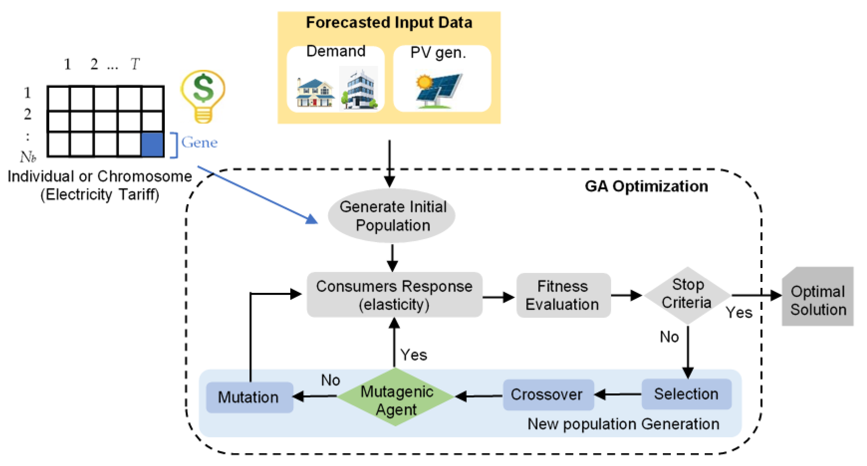
The methodology proposed in this paper consists of an intelligent dynamic pricing scheme for demand response, as shown by the flowchart in
Figure 1. Based on day-ahead forecast profiles of consumer’s demand and PV generation, the optimal electricity tariff is obtained for each consumer group and day hour using the genetic algorithm. The simulation time considered is 24 h with 1 h sampling periods, considering hourly prices are announced 24 h in advance in the market. A population of candidate solutions representing electricity tariffs is generated. Consumer’s demand response associated with each electricity tariff is obtained through elasticity, and fitness function is evaluated to each solution through load flow solutions. Details of the proposed methodology are as follows.
2.1. Mathematic Formulation
This section describes the mathematical formulation of the proposed methodology to achieve optimal electricity price signals to customers at each time of the day, considering the day-ahead market. A multi-objective optimization problem is proposed with the goals: (i) minimize electricity demand fluctuation (
F1), (ii) minimize total load reduction (
F2), and (iii) minimize the average cost of electricity (
F3). The fitness function is formulated as follows.
and each goal is weighted by
w1,
w2, and
w3, respectively.
The term
F1 represents demand fluctuation (
DF), which is the deviation between system electricity demand and system average demand as shown in Equations (2) and (3). The minimization of demand fluctuation aims to obtain a flatter pattern of electricity demand, reducing the discrepancy between peaks and valleys.
where
Lt is the total residual load at time
t obtained in response to the proposed dynamic tariff,
Lt,k is the residual load at time
t at bus
k obtained in response to the proposed dynamic tariff,
Pt,k is the load at time
t at bus
k obtained in response to the proposed dynamic tariff,
PVt,k is the renewable generation at time
t at bus
k,
Lav is the total average load for the entire simulation time horizon
T, and
Nb is the number of buses in the system.
The term
F2 represents total load reduction (
TLR) and expresses the effect of dynamic pricing on system demand curtailment as shown in Equations (4) and (5). The minimization of
TLR promotes solutions where consumers increase their consumption after dynamic pricing, generating more profit for the utility. For underdeveloped countries, an energy consumption increase is associated with a better quality of life since families can make use of basic electrical equipment, such as electric showers, washing machines, and air conditioning.
where
Lot is the total nominal load at time
t and
Lot,k is the nominal load at time
t at bus
k.
The term
F3 represents the average cost of electricity (
AC), which should be minimized to reduce customers’ energy bills, as shown in Equation (6). It is important to mention that overall system improvement must be achieved by optimizing the electricity price, not blindly trying to increase or reduce the electricity price.
where
Tr t,k is the electricity tariff at time
t at bus
k.
The minimization problem is subjected to equality and inequality constraints. Equality constraints represent the non-linear power flow equations as shown in Equations (7) and (8).
where
K is the set of buses adjacent to bus
i (including bus
i),
Nb is the total number of buses in the distribution system,
Pi and
Qi are active and reactive power injected at bus
i,
Gij and
Bij are, respectively, the real and imaginary parts of the nodal admittance matrix.
Inequality constraints represent limits on busbar voltage magnitudes, as shown in Equation (9).
where
Vimin and
Vimax are minimum and maximum allowable voltages, assumed to be, respectively, 0.95 and 1.05 pu in this study.
It is important to mention that F1, F2, and F3 are normalized with respect to their base values for preventing scaling problems when fitness is evaluated. Optimizations are performed evaluating the fitness function with w1 = 0.25, w2 = 0.31, and w3 = 0.44.
2.2. Demand Response Modeling
Energy demand is a commodity sensitive to price variations. Price elasticity (
ε) measures energy demand changes relative to price changes, as shown in (10) [
11].
where
d is demand,
d0 is the initial demand,
p is the electricity tariff, and
p0 is the initial electricity tariff.
Commodities can be elastic or inelastic. The price elasticity of demand is said to be elastic when consumers respond to price variations with a large change in demand. In this case, price elasticity assumes values greater than one. On the other hand, demand is said to be inelastic when consumers almost do not respond to price variations, and in this case, price elasticity values vary from zero to one. In matrix form, consumers’ sensitivity to price variation can be represented as given below in Equation (11) [
11].
where ΔD is a vector with dimension
n × 1 representing demand variation, E is elasticity matrix with dimension
n ×
n, and ΔP is a vector with dimension
n × 1 representing price variation for a pricing system with
n tariff periods.
Demand variation elements are Δdi = di − d0i, where d0i is the initial demand at time i, and di is the corresponding modified demand at time i (after consumers respond to price signals). Price variation elements are Δpi = pi − p0i, where p0i is the initial tariff at time i, and pi is the new tariff at time i.
The elasticity matrix can be represented as shown in Equation (12).
where matrix diagonal terms
εi,i are the self-elasticity coefficients, and matrix off-diagonal terms
εi,j are the cross-elasticity coefficients.
The self-elasticity coefficients describe how consumers react, changing their demand on time at instant i due to price variations occurring at the same instant i, and always assume negative values. The cross-elasticity coefficients describe how consumers change their demand at time instant i based on price variations occurring in another instant j, and always assume positive values (multi-period sensitivity).
Applying a dynamic electricity price at time
i, the responsive electricity demand at time
i can be evaluated as shown in Equation (13), considering its influence in other periods
j [
12].
2.3. Genetic Algorithm (GA)
The genetic algorithm is a meta-heuristic optimization technique inspired in nature, based on Darwin’s theory of natural evolution. GA is a widely used optimization algorithm with many engineering applications, including power systems. It has been successively used to solve complex, non-linear, and multi-objective optimization problems. As a population algorithm, it can escape from local optima if parameters are properly adjusted due to its exploration and exploitation characteristics. GA’s main steps are population initialization, fitness evaluation, and new population generation using GA operators (selection, crossover, and mutation) [
13].
2.3.1. Initialization of Population
In the genetic algorithm, a chromosome (also known as an individual) is characterized by a set of features called genes. The set of all individuals (solutions) is known as the population. In this problem, each individual represents a matrix with Nb lines and T columns, corresponding to the electricity tariff to each node of the system to each hour of the day. These elements are decision variables of the problem and are represented in their natural form (real numbers). To initialize the population, N individuals are randomly created within the feasible range of decision variables. To each individual (new electricity tariffs), the new electricity demand is evaluated considering the cross and self-elasticity effect, and the fitness function is calculated.
2.3.2. Selection
Selection is the procedure where the best individuals are selected based on their fitness value for reproduction in order to produce successive generations. Individuals with high fitness values have a higher probability of being selected. The selection rule used in this paper is roulette-wheel. In roulette wheel selection, the wheel is divided into n pieces, where n is the number of individuals in the population. Each individual gets a portion of the circle that is proportional to its fitness value. Individuals with higher fitness are more likely to be selected.
2.3.3. Crossover
Crossover is a genetic operator used to combine genetic information of two parents to generate new offspring. This study applied single-point crossover. In this case, a random crossover point is selected, and the tail of its two parents is swapped to get new offspring, which belong to the next generation of possible solutions.
2.3.4. Mutagenic Agent
Since crossover replaces chromosomes from parents, new solutions will always present genes from parents that can be future modified by mutation. If there are bad genes within the parents, they will be transferred to their children after crossover. To overcome this limitation, a novel operator called the mutagenic agent is applied. This operator is inspired by the new gene-editing method CRISPR/Cas9 developed by Emmanuelle Charpentier and Jennifer A. Doudna, winners of the 2020 Nobel Prize [
14]. This genetic tool allows scientists to modify DNA, cutting bad genes and replacing them with good ones.
In this study, good and bad genes are identified through empirical knowledge of the problem. Bad genes are those electricity tariffs below the one currently applied (flat tariff) when electricity consumption is higher than the daily average value, promoting an increase in electricity consumption during this peak period. A bad gene could also be an electricity tariff above the one currently applied when electricity consumption is lower than the daily average value, promoting a reduction in electricity consumption during this off-peak period. Good genes have the opposite behavior.
The mutagenic agent will identify bad genes and replace them with better ones. This replacement is represented by a variation in the direction that best satisfies the goal or will assume a new random value, with a chance of 50%. This agent is inserted into the population following a geometric progression of ratio 2, starting at the 15th generation. Thus, there is a strong exploration of the search space in the early generations, visiting new regions and increasing population diversity. At the end of the evolutionary process, there is more exploitation of the search space, reducing the necessity to apply the mutagenic agent.
2.3.5. Mutation
Mutation prevents premature stopping of the algorithm in a local solution. It introduces diversity in the GA population. In this study, a conventional mutation operator is applied with probability within the domain ε [0.1,1.7] to every gene of the chromosome.
Table 1 shows the values adopted for the set of parameters used in the GA in this study after performing extensive statistical tests.
5. Simulation Results
The performance of the proposed method is evaluated through simulations considering the following scenarios:
Case 1 is the base case, which considers the conventional flat tariff and load curve of
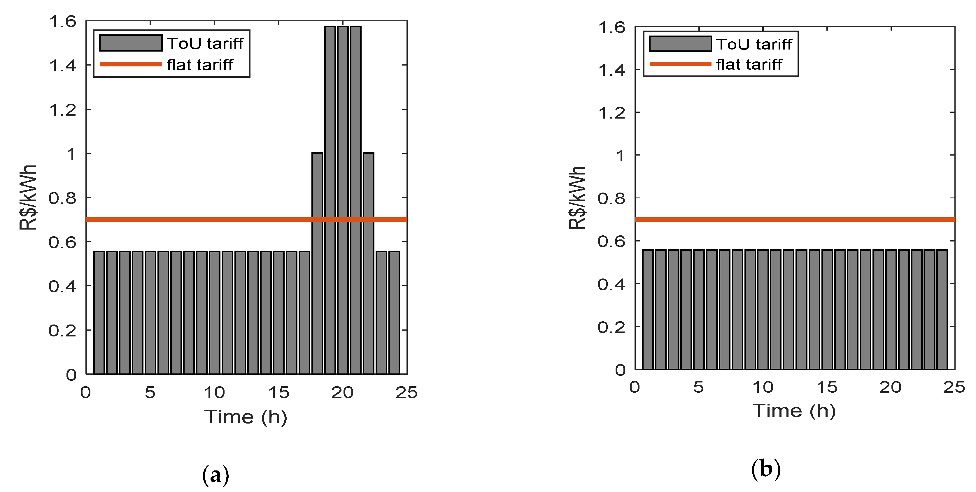
Figure 3, where no DR program is implemented. In Case 2, energy demand is evaluated in response to the White tariff combined with the price elasticity concept. In Case 3, the proposed IDP method is applied to obtain a dynamic tariff, and energy demand is evaluated in response to the new tariff considering price elasticity.
Simulations are conducted using MATLAB toolbox, and power flow simulations are performed using MATPOWER toolbox [
22,
23]. The proposed methodology is applied to the test system, and results are obtained considering both the original system and its modified version with the integration of renewable energy sources. The demand response is indicated separately, by the consumer side and by the utility side. Considering the consumer side, the following technical aspects are analyzed: daily energy consumption and average electricity cost. The utility side results are evaluated in terms of utility profit, peak load reduction, and load factor (the average load divided by the peak load in a specified period, indicating the efficiency of electrical energy usage).
5.1. Original System
Table 3 shows the results obtained for all three cases analyzed considering the original test system. When consumers adhere to the ToU tariff (Case 2), the average electricity tariff paid by customers slightly increases to BRL 0.7205, which is not favorable to them. On the other side, energy consumption increases, indicating better quality of life for clients. Utility profit increases to BRL 34,864.00, load factor increases to 0.74, and peak demand is reduced by 5.28%. When the intelligent dynamic pricing method (Case 3) is applied, the average electricity tariff paid by customers slightly reduces to BRL 0.6900, and the client’s energy consumption increases. The utility also has advantages, such as greater profit (BRL 36,067.00), greater peak demand reduction (9.63%), and more efficient use of energy with a greater increase in load factor (0.77). The proposed scheme is favorable for both utility and consumers in all aspects, offering more attractive results when compared to flat and ToU tariffs.
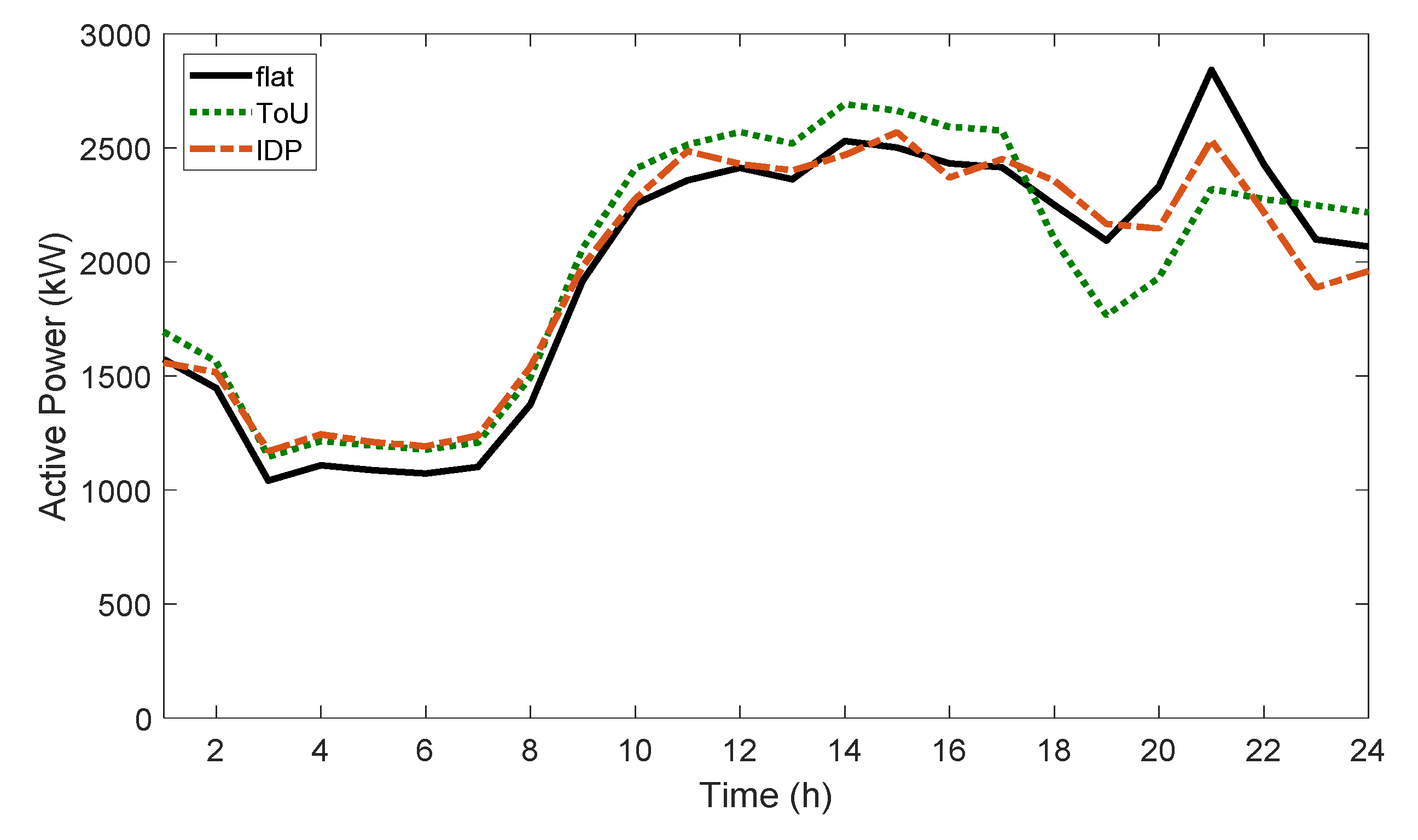
Figure 7 shows the impact of different tariffs on the total load curve. Results show the ToU tariff (Case 2) causes the undesirable rebound effect, resulting in another peak demand at 14:00 h. This effect is not observed with IPD, which only reduces peak demand.
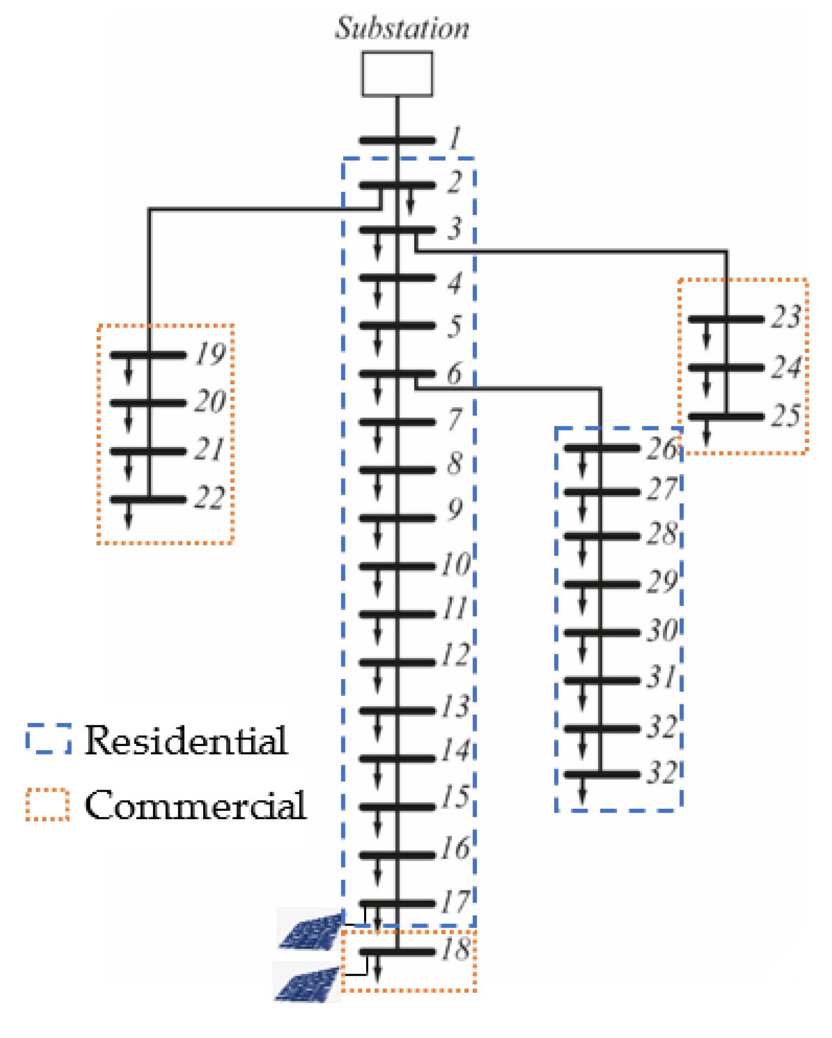
Figure 8 shows electricity tariffs obtained applying the proposed method at buses 17 and 18, which are residential and commercial customers, respectively. The proposed IDP scheme generates electricity tariffs for each type of customer, commercial and residential. For commercial consumers, electricity tariffs tend to be more expensive during peak hours, which is around noon, differently from the ToU tariff, which has a fixed price for everyone.
5.2. Renewable Energy Integration
In this section, the behavior of the proposed methodology is evaluated considering the integration of renewable energy sources in the original system.
Table 4 shows results obtained for all three cases. Adopting the flat tariff, the connection of PV generation reduces utility profit from 32,987.97 (see
Table 1) to BRL 26,970.97, due to a decrease in energy consumption from 47,125.67 (see
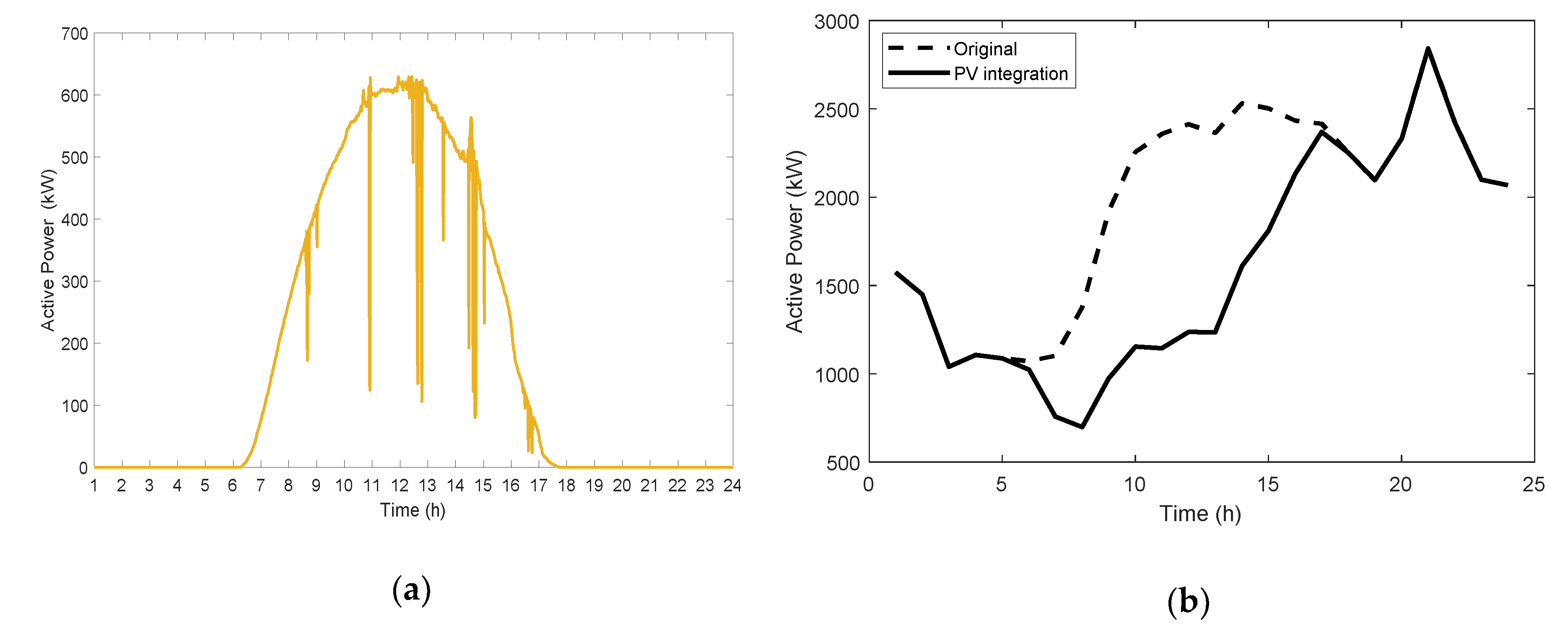
Table 1) to 38,530.30 kWh. Since the availability of PV generation does not coincide with demand peak hours, peak load is sustained at 2843.10 kW.
The adoption of the ToU tariff reduces utility financial loss, increasing energy consumption to 39,570.00 kWh and utility profit to BRL 30.084,00. The load factor increases from 0.56 to 0.65, and peak demand is reduced by 10.95%. However, the average electricity tariff paid by customers increases from 0.7 to BRL 0.7205. With the adoption of the proposed dynamic tariff IDP, utility profits increase and peak demand reduction is more expressive, achieving values of BRL 31,067.00 and 11.34%, respectively. The load factor increases to 0.65, equal to the ToU tariff, and energy consumption increases to 39,294.00 kWh. The proposed solution offers customers an average electricity tariff cheaper than the flat tariff and ToU tariff of BRL 0.6857.
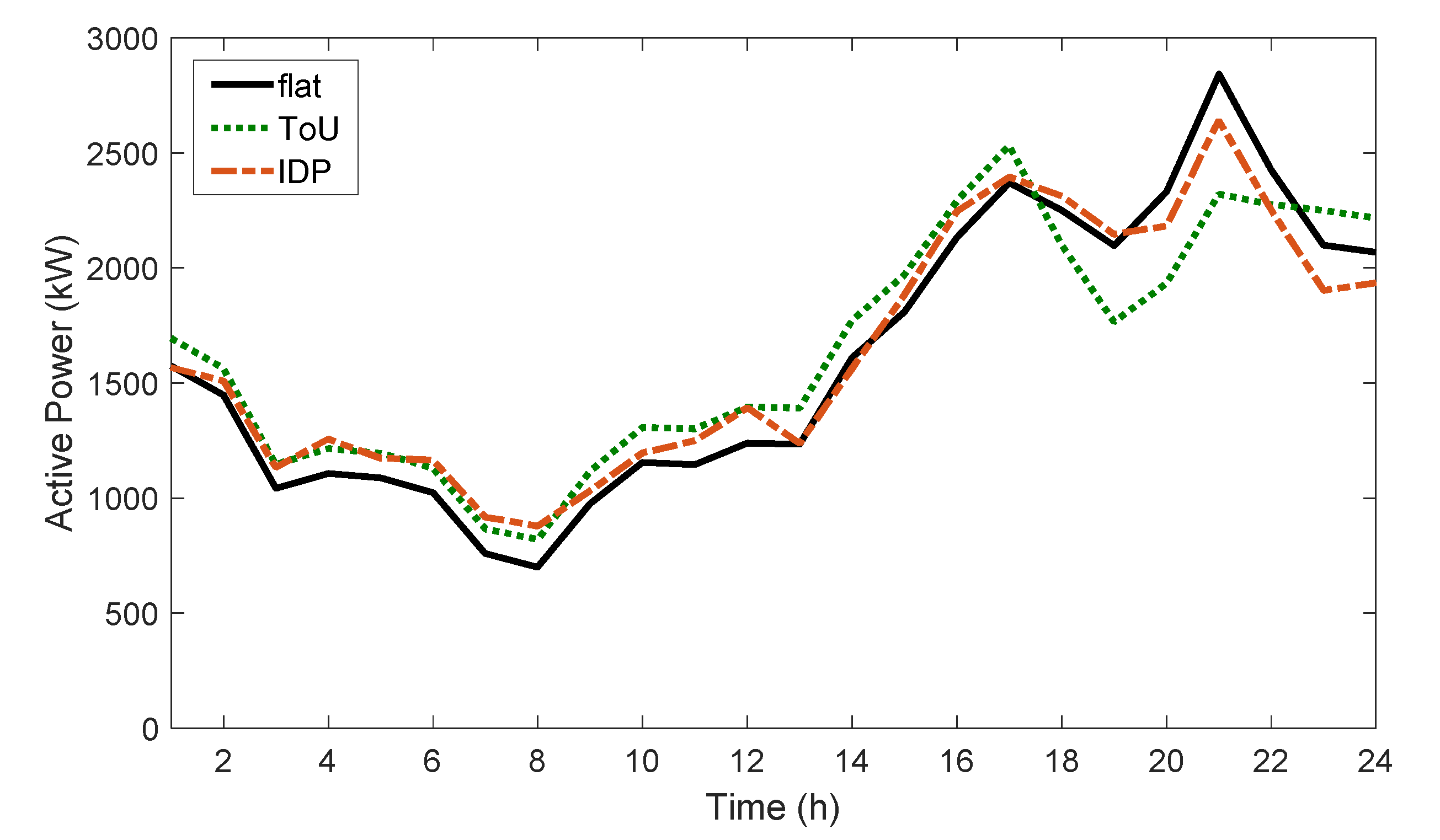
Figure 9 shows the impact of different tariffs on the load curve when PV generation is connected. The use of a dynamic tariff results in a flatter load curve profile without the rebound effect.
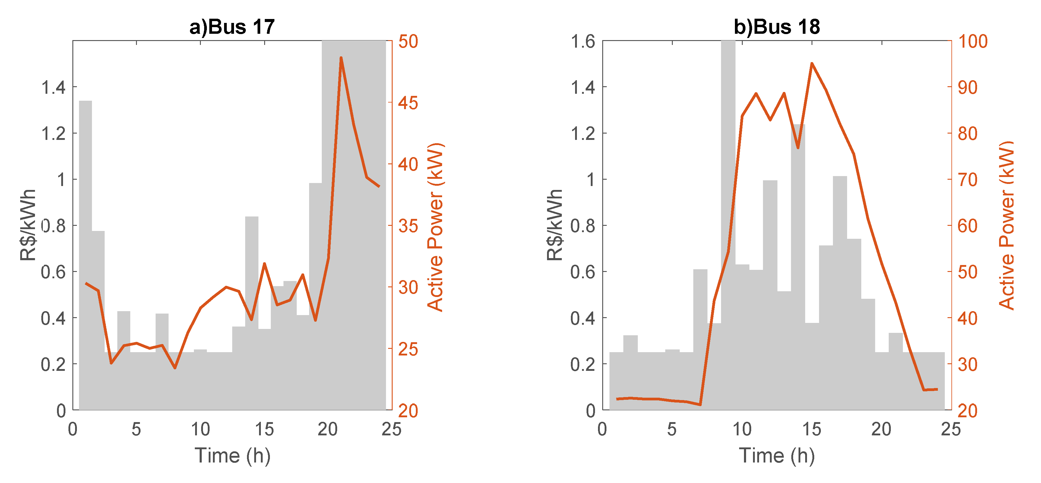
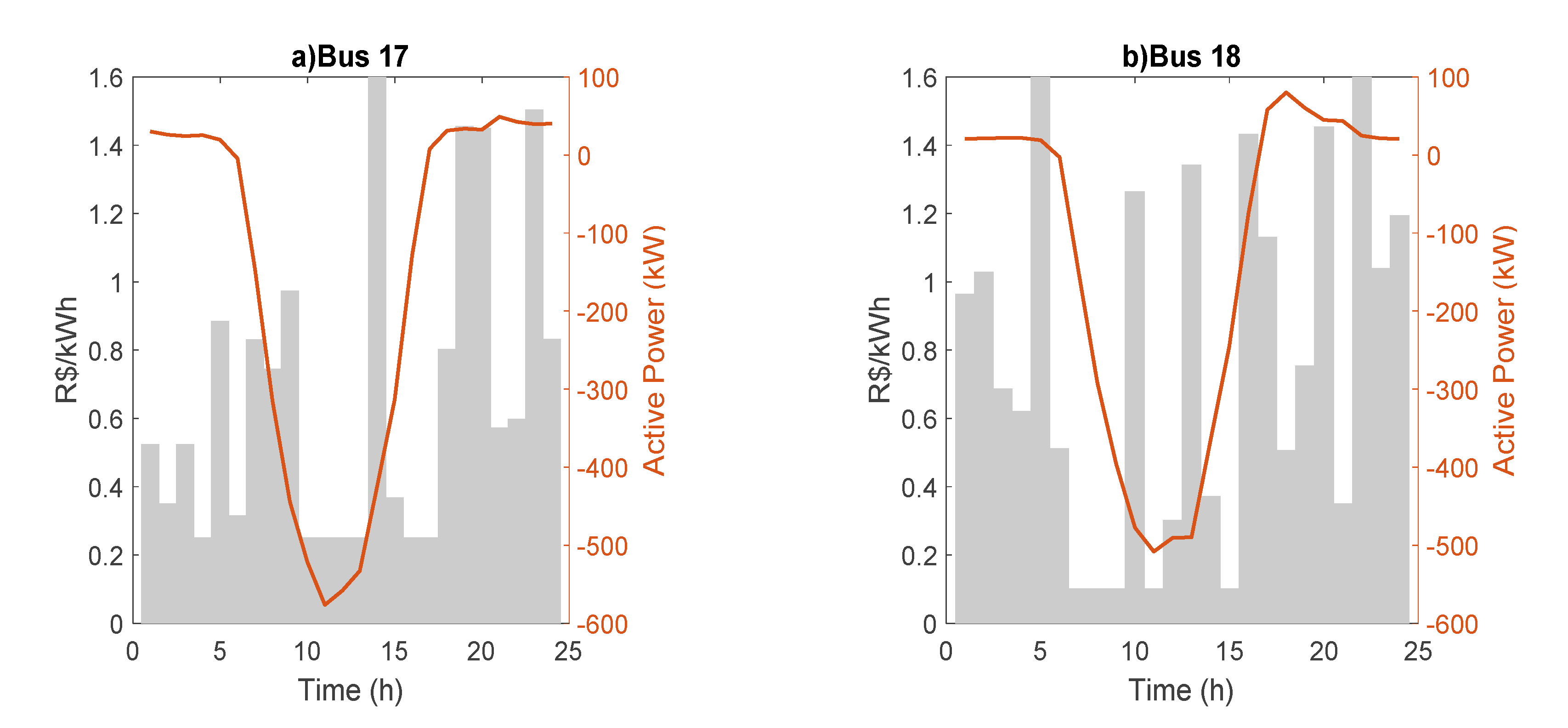
Figure 10 shows demand at nodes 17 and 18, in which PV generation was installed in response to a dynamic tariff. Note that when PV generation is available (mostly between 8:00 h and 15:00 h), the dynamic tariff is low for both commercial and residential clients, acting as a consumption incentive during those hours. The dynamic tariff adapts to the presence of PV generation and creates incentives to increase consumption when it is available through cheaper tariffs, changing the costumer’s consumption profile. The application of an intelligent dynamic tariff improves system performance and helps the utility to postpone investments.
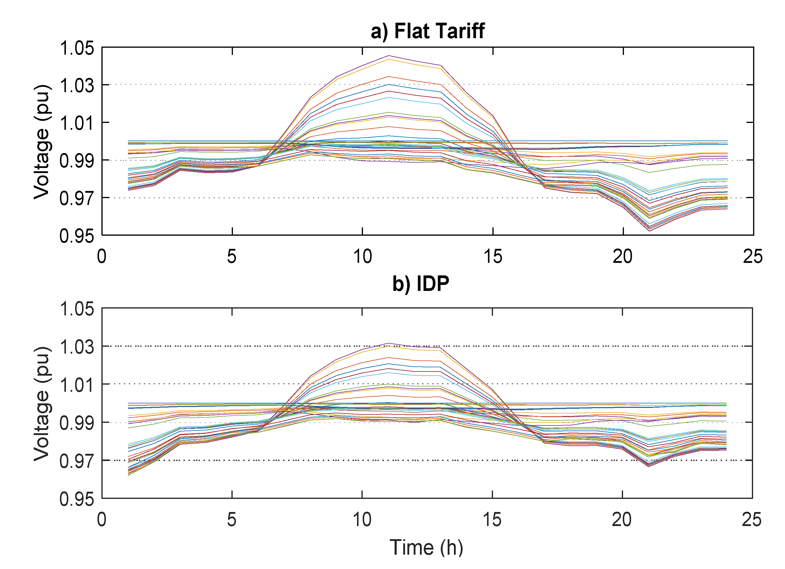
Figure 11 shows active power flow is reduced in most distribution lines, relieving congestion. Further, the system voltage profile is improved, as shown in
Figure 12.
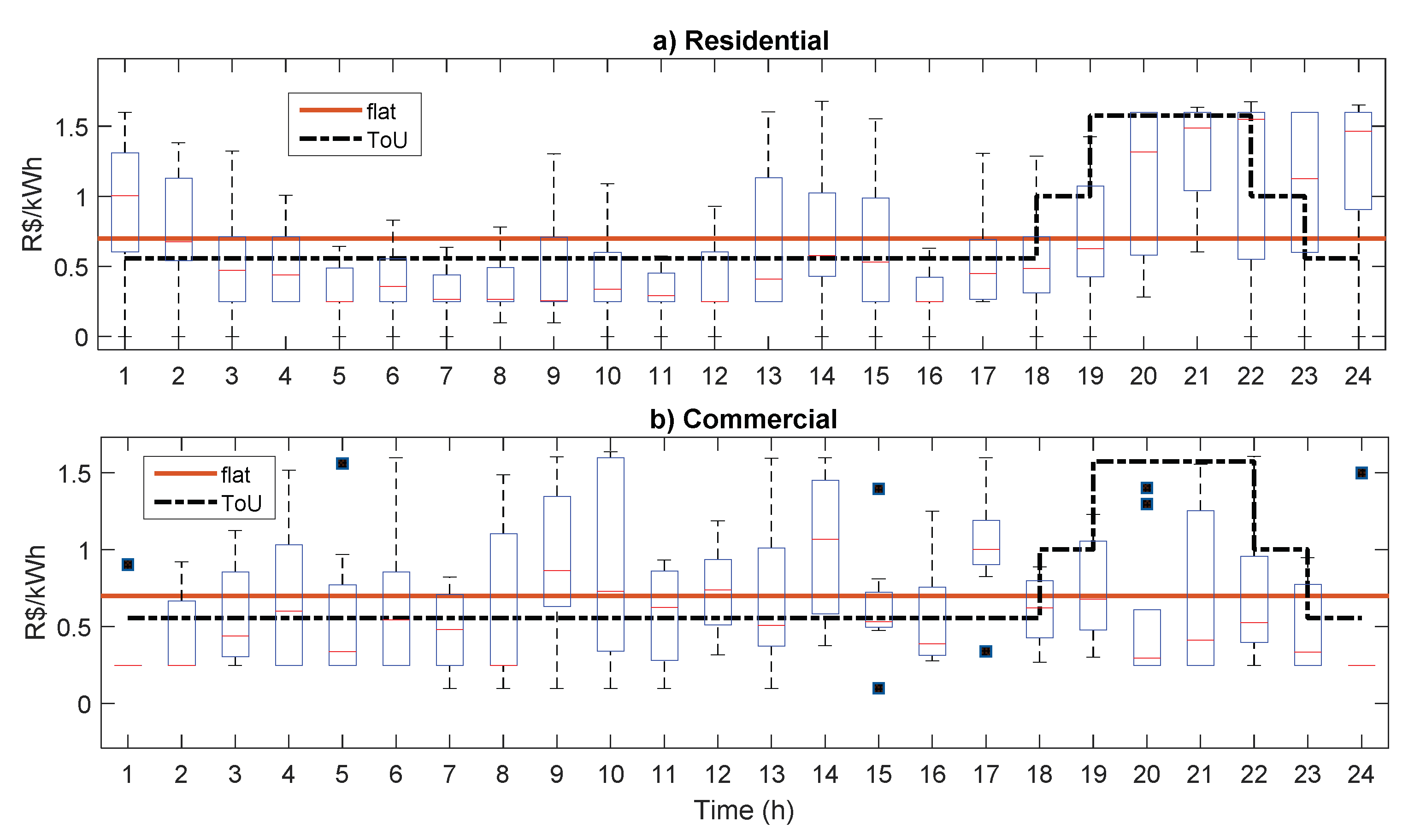
Figure 13 shows the boxplot of the proposed dynamic tariff, compared with flat and ToU tariffs adopted in the Brazilian market. In the boxplot, the line dividing the box indicates the median, the edges of the box show 25th and 75th percentiles of data, and the ‘whiskers’ extend to include all data. The variability of the dynamic tariff to each bus along the day can be verified. Commercial customers have higher tariff variability during the day when their demand is higher. This is caused by the predominance of flexible loads (refrigeration) in these types of consumers [
24]. These loads allow a bigger variation in demand, which ends up influencing tariff values offered.
5.3. Algorithm Convergence Discussion
The proposed dynamic pricing uses a metaheuristic algorithm, and convergence is an especially relevant issue. It is important to conduct statistical performance evaluations to analyze the progress of the optimization process.
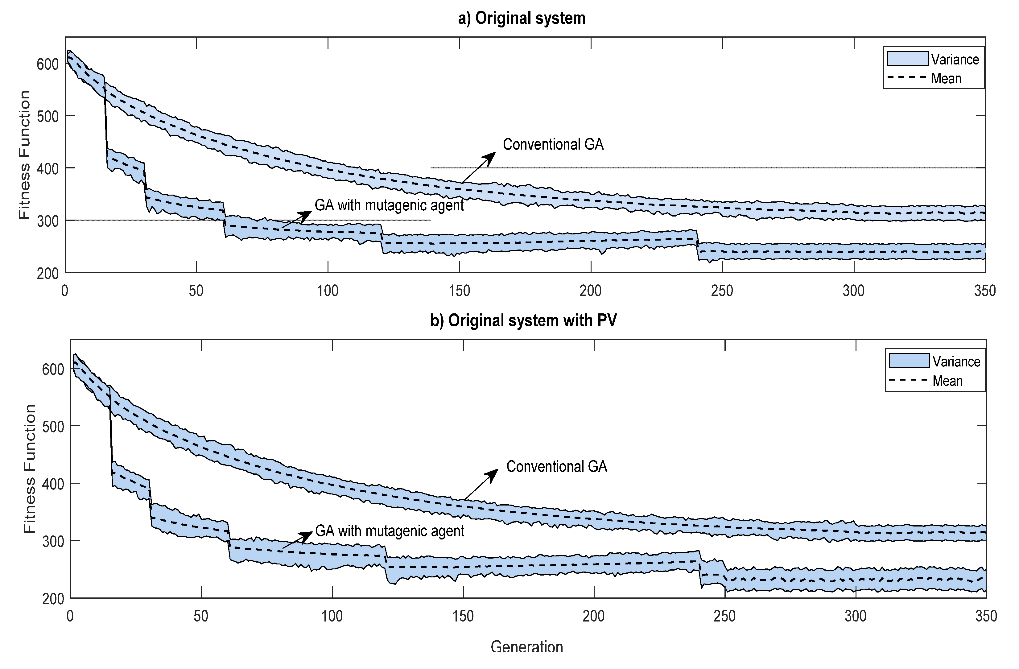
Figure 14 shows the mean and variance of the best fitness function values over 300 generations for 100 experiments (10 trials of each 10 different initial populations) obtained with the original GA and the proposed GA with the mutagenic agent for comparison purposes. Both scenarios are considered: the original system with and without the integration of PV generation.
Based on the simulation results, it is observed that the mutagenic agent has a strong intensification effect that directs the population more quickly to the optimal solution, introducing a bias in the population through good genes, reducing fitness function. The proposed GA with the mutagenic agent reaches its optimal solution around the 250th generation with a fitness function equal to 228, and further evolution of the population did not show any significant improvement on the objective function, while the conventional GA reaches fitness function equal to 314 after 250 evaluations. The proposed GA with the mutagenic agent brings improvement on exploitation capability of conventional GA, with positive results when applied to this problem, accelerating convergence and finding a better solution.
6. Conclusions
This paper proposed an intelligent dynamic pricing methodology for demand response in distribution systems with the integration of renewable energy sources. An elasticity concept is applied, and segmentation of the electricity market is performed based on consumer type (residential and commercial). The proposed method was modeled as a multi-objective problem, simultaneously optimizing demand fluctuation, the average cost of electricity, and the client’s energy consumption. The genetic algorithm was applied to solve the problem, and a novel operator called the mutagenic agent was proposed, obtaining dynamic tariffs for each day hour and consumer type.
The results of the proposed dynamic pricing scheme are compared with two tariffs adopted in Brazil: a flat tariff and a ToU tariff. Simulations were conducted in the IEEE 33-bus system, using demand and elasticity data from Brazil. According to the results, for the supply side, the proposed dynamic tariff increased load factor and utility profit, and peak demand reduced more significantly. A flatter demand curve was obtained without the undesirable rebound effect. Further, the voltage profile was improved, and line flow congestion was reduced. For the demand side, dynamic tariff resulted in a cheaper average electricity tariff, increasing energy consumption. When PV generation was inserted in the system, the results were favorable for both the utility and customer, indicating the proposed dynamic tariff scheme facilitates the integration of renewable energy with a win-win framework. Regarding the performance of the proposed algorithm, the results are compared with the conventional GA and show the mutagenic agent significantly improves the conventional GA, with better performance not only in terms of convergence but also in terms of fitness function accuracy.


