Assessing the Energy, Indoor Air Quality, and Moisture Performance for a Three-Story Building Using an Integrated Model, Part Two: Integrating the Indoor Air Quality, Moisture, and Thermal Comfort

Abstract

In this paper, an integrated model that coupled CONTAM and WUFI was developed to assess the indoor air quality (IAQ), moisture, and thermal comfort performance. The coupling method of CONTAM and WUFI is described based on the exchange of airflow rate control variables as infiltration, natural and mechanical ventilation parameters between heat and moisture flow balance equations in WUFI and contaminant flow balances equations in CONTAM. To evaluate the predictions of the integrated model compared to single models of CONTAM and WUFI, four scenarios were used. These scenarios are airtight-fan off, airtight-fan on, leaky-fan off, and leaky-fan on, and were defined for a three-story house subjected to three different climate conditions of Montreal, Vancouver, and Miami. The measures of the simulated indoor CO₂, PM_2.5, and VOCs obtained by CONTAM; the simulated indoor relative humidity (RH), predicted percentage of dissatisfied (PPD), and predicted mean vote (PMV) obtained by WUFI; and those obtained by the integrated model are compared separately for all scenarios in Montreal, Vancouver, and Miami. Finally, the optimal scenarios are selected. The simulated results of the optimal scenarios with the integrated model method (−28.88% to 46.39%) are different from those obtained with the single models. This is due to the inability of the single models to correct the airflow variables.

1. Introduction

A building can be defined as a system that balances the energy, air, and moisture flows with its surroundings. Indoor air quality, moisture, and thermal comfort are important parameters for buildings that can be controlled based on energy, air, and moisture flows characteristics. Currently, there are many tools that can be used for determining energy, indoor air quality, and moisture building performances. Residents’ satisfaction with the thermal condition of the indoor environment increases the performance of the buildings [1]. Energy models are accurate tools for optimizing active and passive building systems [2,3,4].

Thermal comfort measures have been developed since the 1960s to calculate building performance and the predicted mean vote (PMV) has been used as one of the numerical measures of thermal comfort [5]. ASHRAE Standard 55 [6] is one of the most important international thermal comfort standards. Many tools have been developed by researchers to calculate thermal comfort as an indicator of building performance. Some of these tools such as FTCR (Functions for Thermal Comfort Research) [7] and pythermalcomfort [8] are open source tools that require prior coding skills.

Another tool called the Center for the Built Environment (CBE) was developed by Tartarini et al. [9] that can visually calculate the thermal comfort measures according to the ASHRARE 55 standard without the need for having to write code. Chen [10] used indoor air quality calculation tools to calculate building indoor air quality performance. It has been concluded that CFD models were the most popular and can be coupled with other ventilation models to increase their accuracy in calculating the indoor air quality performance of a building. In another study, Wang and Chen [11] concluded that with the help of coupling CONTAM with CFD models, the errors created by some assumptions can be solved and they validated their results with experimental data.

Some researchers have used the coupling method between energy models with indoor air quality models to increase the accuracy of performance calculation for the double skin facade system in natural ventilation [12]. Gao et al. [13] developed a high-precision model by combining thermal comfort and indoor air quality (IAQ) models.

Chang et al. [14] used WUFI (Wäme und Feuchte instationär) Pro 5.3 [15] to perform a moisture risk assessment based on a hygrothermal properties analysis for the ply-lam cross-laminated timber (CLT) house envelope. The WUFI program can calculate the thermal and moisture properties of a building material as hygrothermal performance by calculating heat and moisture flow balances [16]. The performance calculation of thermal and moisture properties of building materials using WUFI tools was performed in 2003 by Canada Mortgage and Housing Corporation for more than 45 building simulation programs [17]. In most studies, WUFI tools were used to minimize moisture problems in preventing mold growth risk at indoor envelope surfaces in order to calculate moisture performance [18]. The problem with moisture performance simulation tools for building materials is that these tools can only estimate hygric behavior and do not predict pollutant behavior, for example, for building materials with a moisture buffering capacity [19]. Relative humidity (RH) is the main parameter needed for evaluating thermal comfort and moisture performance. One of the passive methods to keep moisture in the acceptable level in order to improve thermal comfort is to use building materials with a moisture buffering capacity [20]. Some researchers have concluded that building materials such as gypsum board, ceiling tiles, furniture, and carpet with adsorption/desorption capability of indoor VOCs can affect the indoor air quality [21] Hemp concrete is one of the materials with high moisture buffering capacity that with hygric and pollutant behavior can increase the performance of a building in terms of moisture and IAQ, as well as thermal comfort [22]. Researchers have concluded that this dual behavior of porous media materials is due to the similarity between the properties of moisture transfer and indoor contaminants such as VOCs [23].

Le et al. [19] developed a coupled moisture, air, and pollutant transport model. In that model, the similarity between adsorption/desorption effects for moisture and VOCs was presented by materials with the potential of buffering capacity, which relative humidity and temperature can affect both.

According to the literature review’s results, it can be concluded that because of temperature, airflow, and the relative humidity (RH) on each of the measures of thermal comfort, indoor air quality, and moisture performance, all three measures need to be integrated to allow for simultaneous correction for the common variables. The study of the results of the single research session of the CONTAM [24,25,26] and WUFI [27,28,29] models concluded that there is a need to develop an integrated model for a more accurate calculation of building indoor air quality, moisture, and thermal comfort performances.

In this research project, an integrated model is developed, in which the first part, related to coupling the energy and indoor air quality, was presented in a previous paper [30]. This paper presents the second part of the research project related to the development of the integrated model to couple the indoor air quality, moisture, and thermal comfort performances. In addition, the results obtained with single models (i.e., CONTAM [31] and WUFI [32]) are compared with those obtained with the present integrated model.

The innovation of this research project is the development of a new model with integrated indoor air quality, moisture, and thermal comfort performance predictions with high accuracy. The accuracy of this integrated model was verified using a paired sample t-test. This method was performed by Heibati et al. [2,3,33] for integrated energy models. Single models’ predictions are made separately for indoor air quality performance or moisture, while thermal comfort performances and airflows with its dependent variables are defined as input data by the user [32,34]. In the integrated model, however, airflows are exchanged and modified as control variables between CONTAM and WUFI sub models. The reason for this advantage of airflows is due to the integrated calculation of heat, moisture, and contaminant equation balances. Finally, the interactions between the indoor air quality, moisture, and thermal comfort performances are balanced and the accuracy of the predictions of this new model is increased.

2. Methodology

An integrated model is developed to simultaneously assess the building performance related to: (1) indoor air quality and (2) moisture with thermal comfort. For this purpose, two single models of CONTAM (ContamW and ContamX, version: 3.2.0.2) [31] and WUFI (WUFI Plus, version: 3.2.0.1) [32] are used. In the first phase, the capability of each of the CONTAM and WUFI models for a case study is evaluated. In the second phase, with the help of coupling method, an integrated model is developed to calculate simultaneously the performance of indoor air quality, moisture, and thermal comfort.

For this purpose, the approach used in this study consists of three sections. Section 1 describes the coupling method of CONTAM and WUFI. In Section 2, the governing equations of the single models as well as the coupling equation are described. In Section 3, a case study is conducted to compare the building performance obtained with the single models and the integrated model at the three different climates of Montreal, Vancouver, and Miami.

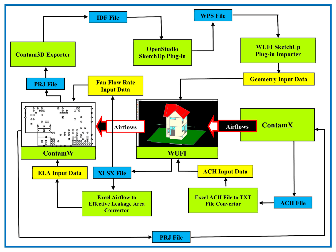
2.1. Coupling Method of CONTAM and WUFI

The coupling mechanism of the two CONTAM and WUFI models is conducted by exchanging control variables and converting the output and input data formats of each model. When one or more output variables can act as readable input for another model and vice versa, and because of this exchange, the variable(s) is/are updated. This process is called a co-simulation mechanism, which is presented in Figure 1. The main variable in this study is airflow rate and the sub-variable is geometry data, which are exchanged between both CONTAM and WUFI models according to Figure 1.

CONTAM mainly consists of two separate programs. These two programs are: 1-ContamW and 2-ContamX. ContamW provides a graphical interface for the user to view the results simulated by ContamX. ContamX can simulate files in PRJ file (project file) format. After entering graphical and numerical data by the user through ContamW, this data is stored in the format of PRJ files. It is then provided as an input file to ContamX for processing and simulation, and finally these results can be viewed graphically through ContamW.

In the airflow rate exchange between CONTAM and WUFI, the output of the air change rate simulated by ContamX [31] in an ACH (air change rate) file format is first converted to a TXT (text) file format by Microsoft Excel. This simulated output contains daily and average annual data for airflow through the paths and ducts. After changing the format, this output is provided to WUFI as input information. In WUFI, this data is used in the natural and mechanical ventilations. The airflow rate outputs simulated by WUFI, which include updated hourly ventilations data, are then converted to an XLSX (Excel Workbook) file via the Excel exporter menu, after which the natural and mechanical ventilations parts are separated. In ContamW [31], the airflow element models selected for the infiltration and mechanical ventilation are the leakage area of the power law model and the constant mass flow fan model, respectively [35]. WUFI output data related to the mechanical ventilation part is then used as the design flow rate of the fan model according to Figure 1. The natural ventilation–infiltration air–volume flow rate ($\dot{Q}$) as an output part is converted to ELA (effective leakage area) by the Excel convertor airflow to ELA, based on the converter factor, and then used as an input data leakage area model of ContamW. The converter factor tool is executed according to Equations (1)–(3) [36,37].

$$ACH=\frac{\left(3600\times \dot{Q}\right)}{V}$$

(1)

$$NL=ACH$$

(2)

$$NL=1000·\frac{ELA}{A_f}·{\left(\frac{H}{2.5}\right)}^{0.3}$$

(3)

where $ACH$, $\dot{Q}$, $V$, $NL$, ELA, $A_f$, and H correspond to the air change rate (h⁻¹), natural ventilation–infiltration air–volume flow rate (m³/s), building net volume (m³), normalized leakage, effective leakage area, floor area (m²), and building height (m), respectively.

It is assumed in WUFI that the natural ventilation–infiltration air–volume flow rate is a function of the internal and external temperatures’ difference. The reason for this relationship is presented according to Equations (4)–(6). The natural ventilation–infiltration air–volume flow rate is calculated based on the amount of heat flow from natural ventilation–infiltration according to Equations (4) and (5). Conversely, heat flow from natural ventilation–infiltration is a function of the internal and external temperatures’ difference based on Equations (4) and (5) [38].

$${\dot{m}}_{nat-infiltration}=\dot{Q}·\rho$$

(4)

$${\dot{q}}_{nat-infiltration}={\dot{m}}_{nat-infiltration}·\left(h_i-h_e\right)$$

(5)

$$h_i-h_e=\left(1006+x_e·1840\right)·\left({\theta }_i-{\theta }_e\right)$$

(6)

In Equations (4)–(6), ${\dot{m}}_{nat-infiltration}$, $\rho$, ${\dot{q}}_{nat-infiltration},$ $h_i$, $h_e$, $x_e$, ${\theta }_i$, and ${\theta }_e$ correspond to the airflow of natural ventilation–infiltration (kg/s), air density of internal air (kg/m³), heat flow from natural ventilation–infiltration (W), specific enthalpy internal air (J/kg), specific enthalpy external air (J/kg), moisture content of external air (kg/kg), internal air temperature (°C), and external air temperature of (°C), respectively.

In this coupling method, it is assumed that in the ContamW sub model section, the infiltration model is based on the following empirical (power law model [39]) relationship between the natural ventilation–infiltration air–volume flow rate and the pressure difference across a crack or opening in the building envelope (see Equation (7)). ContamW is able to calculate natural ventilation–infiltration air–volume flow using the power law model in Equation (7) and by using the component leakage area formulation through Equations (8) and (9) [39], which has been used to characterize openings for infiltration calculations. Equation (8) presents the relationship between ELA and a series of pressurization tests in which the airflow rate is measured at a series of reference condition pressures. Conversely, ELA relates to the natural ventilation–infiltration air–volume flow rate based on the power law model through Equations (7)–(9).

$$\dot{Q}=C·{\left(\Delta P_r\right)}^n$$

(7)

$$ELA={\dot{Q}}_r·\frac{\sqrt{\frac{\rho }{2·\Delta P_r}}}{C_d}$$

(8)

$$C=ELA·C_d·\sqrt{2}·{\left(\Delta P_r\right)}^{\frac{1}{2}-n}$$

(9)

In Equations (7)–(9), $C$, $\Delta P_r$, n, ${\dot{Q}}_r$, and $C_d$ correspond to the flow coefficient (m³/(s·Paⁿ)), reference pressure difference (Pa), flow exponent, predicted airflow rate at $\Delta P_r$ (m³/s) (from curve fit to pressurization test data), and discharge coefficient. There are two sets of reference conditions for the discharge coefficient: $C_d=1 \mathrm{and} \Delta P_r=4 \left(\mathrm{Pa}\right)$ or $C_d=0.6 \mathrm{and} \Delta P_r=10 \left(\mathrm{Pa}\right)$ [39]. Additionally, the effective leakage area is used in ContamW at a pressure difference ($\Delta P_r$) of 4 Pa, flow exponent (n) of 0.65, and discharge coefficient ($C_d$) of 1 [37]. According to Figure 1, both WUFI and CONTAM models use the simulated airflow rate simulation data instead of the assumed input variable of airflow rate. Consequently, the co-simulation for this main control variable is completed.

In the next step, the geometry data simulated by ContamW is converted from a PRJ file (project file) to a IDF file (input data file) with the help of Contam3D Exporter. The IDF file can be read by the importer of OpenStudio SketchUp Plug-in and the details of this geometry can be controlled and modified. It is then read as a WPS file (WUFI Plugin in SketchUp file) by WUFI SketchUp Plug-in importer as an input geometry file to WUFI. In this procedure, the simulated geometry data is controlled and modified as a sub-variable by CONTAM in Sketchup, and then is used as input data in WUFI. Finally, the exchange of both the airflow rate and geometry control variables, as shown in Figure 1, between CONTAM and WUFI completes the co-simulation process in this part of the study.

The governing equations of the integrated model, which include the coupling of the flow rates of heat, moisture, and contaminant, are provided by Equations (10)–(12) [35,40]. Equations (10) and (11) provide the heat and moisture balance equations by WUFI, respectively. Equation (12) represents the contaminant flow balance equation by CONTAM in this combination.

$$\frac{d{Q}_{heat,i}}{dt}={{\displaystyle \sum }}_j{\dot{q}}_{component,j}^{opaque}+{{\displaystyle \sum }}_j{\dot{q}}_{component,j}^{transparent}+{\dot{q}}_{solar}+{\dot{q}}_{internal}+{\dot{q}}_{nat-infiltration}+{\dot{q}}_{mech-ventilation}$$

(10)

$$\frac{d{W}_{moist,i}}{dt}={{\displaystyle \sum }}_i{\dot{w}}_{component,j}+{\dot{w}}_{indoor}+{\dot{w}}_{nat-infiltration}+{\dot{w}}_{mech-ventilation}$$

(11)

$$\frac{d{m}_{cont,i}^{\alpha }}{dt}={\displaystyle \sum }_j{\dot{m}}_{air-inwar{d}_{\left(j,i\right)}}·\left(1-{\eta }_{j, i}^{\alpha }\right)·C_j^{\alpha }+G_i^{\alpha }+m_{ai{r}_i}{\displaystyle \sum }_{\beta }{K}_i{}^{\alpha ,\beta }·C_i^{\beta }-{\displaystyle \sum }_j{\dot{m}}_{air-outwar{d}_{\left(i,j\right)}}·C_i^{\alpha }-R_i^{\alpha }·C_i^{\alpha }$$

(12)

In Equation (10), $\frac{d{Q}_{heat,i}}{dt}$, ${\dot{q}}_{component,j}^{opaque}$, ${\dot{q}}_{component,j}^{transparent}$, ${\dot{q}}_{solar}$, ${\dot{q}}_{internal}$, ${\dot{q}}_{nat-infiltration}$, and ${\dot{q}}_{mech-ventilation}$ correspond to the heat flow rate in zone i (room) (W), heat transfer flow over opaque component j (W), heat transfer flow over transparent component j (W), short-wave solar radiation leading directly to heating the internal air or interior furnishing and components surface (W), convective heat sources in the room (W), heat flow from the natural ventilation–infiltration (W), and convective heat flow from the building mechanical ventilation systems (W), respectively [40].

In addition, in Equation (11), $\frac{d{w}_{moist,i}}{dt}$, ${\dot{w}}_{component,j}$, ${\dot{w}}_{internal}$, ${\dot{w}}_{nat-infiltration}$, and ${\dot{w}}_{mech-ventilation}$ correspond to the moisture flow rate in zone i (kg/s), moisture flow between inner wall surface j and the room air (kg/s), moisture source in the room (kg/s), moisture flow due to the natural ventilation–infiltration (kg/s), and moisture flow due to the building mechanical ventilation systems (kg/s), respectively [40].

In Equation (12), $\frac{d{m}_{cont,i}^{\alpha }}{dt}$, ${\dot{m}}_{air-inwar{d}_{\left(j,i\right)}}$, ${\dot{m}}_{air-outwar{d}_{\left(i,j\right)}}$, $C_i^{\alpha }$, $C_i^{\beta }$, $C_j^{\alpha }$, $G_i^{\alpha }$, $m_{ai{r}_i}$, ${\eta }_{j,i}^{\alpha }$, $K_i{}^{\alpha ,\beta }$, and $R_i^{\alpha }$ correspond to the contaminant of $\alpha$ flow rate in zone i (kg/s), inward flow rate of air from zone j to zone i (kg/s), outward flow rate of air from zone i to zone j (kg/s), concentration of contaminant $\alpha$ in zone i (kg/kg), concentration of contaminant $\beta$ in zone i (kg/kg), concentration of contaminant $\alpha$ in zone j (kg/kg), generation rate of contaminant $\alpha$ in zone i (kg/s), mass of air in zone i (kg), filter efficiency for contaminant $\alpha$ in the path from zone j to zone i, kinetic first order chemical reaction coefficient in zone i between contaminant $\alpha$ and $\beta$ (s⁻¹), and removal coefficient of contaminant $\alpha$ in zone i (kg/s), respectively [35].

The variables dependent on the heat flow rate in zone i ($\frac{d{Q}_{heat,i}}{dt}$) are calculated based on Equations (13)–(21) [40]. A transmission heat flow over opaque component j (${\dot{q}}_{component,j}^{opaque}$) is calculated based on Equation (13). In this equation, $A_C$, $R_{si}$, ${\theta }_i$, and ${\theta }_{si}$ correspond to the surface of the opaque component (m²), heat transfer resistance interior (m²·K/W), internal room air temperature (°C), and interior surface temperature (°C), respectively.

$${\dot{q}}_{component,j}^{opaque}=A_C·\frac{1}{R_{si}}·\left({\theta }_i-{\theta }_{si}\right)$$

(13)

In addition, a transmission heat flow over transparent component i (${\dot{q}}_{component,j}^{transparent}$) is calculated based on Equation (14).

$${\dot{q}}_{component,j}^{transparent}=\left[\left({\theta }_e-{\theta }_i\right)-E·\left(I_{l,e}-\sigma ·T^4\right)·R_e+I_{l,i}·R_i\right]·U_W·A_W$$

(14)

In Equation (14), ${\theta }_e$, $E$, $I_{l,e}$, $I_{l,i}$, $\sigma$, $T$, $R_e$, $R_i$, $U_w$, and $A_w$ correspond to the external temperature (°C), emissivity (average of glazing and frame), long-wave radiation balance of exterior surface (W/m²), long-wave radiation balance of interior surface (W/m²), Stefan Boltzmann constant 5.67⋅10⁻⁸ (W/m²⋅K⁴), temperature of the exterior surface (K), heat transfer resistance, exterior (m²⋅K/W), heat transfer resistance, interior (m²⋅K/W), heat transfer coefficient of the entire window (W/m²·K), and total surface area (window frame + glazing) (m²), respectively. In Equation (15), short-wave solar radiation (${\dot{q}}_{solar}$) (W) is calculated by the summation of ${\dot{q}}_{solar,i}$ and ${\dot{q}}_{solar,c}$, which are solar-gain for the internal air or interior furnishing (W), and solar-gain for the components surface (W), respectively.

$${\dot{q}}_{solar}={\dot{q}}_{solar,i}+{\dot{q}}_{solar,c}$$

(15)

$${\dot{q}}_{solar,i}=f_{sa}·{\dot{q}}_{solar,G}$$

(16)

$${\dot{q}}_{solar,c}=\left(1-f_{sa}\right)·{\dot{q}}_{solar,G}$$

(17)

$${\dot{q}}_{solar,G}={{\displaystyle \sum }}_w[(I_{s, dir}·f_{sh,dir}·SHG{C}_{dir}+I_{s,diff}·f_{sh,diff}·SHG{C}_{diff})·A_w·f_f$$

(18)

Both ${\dot{q}}_{solar,i}$ and ${\dot{q}}_{solar,c}$ are calculated based on Equations (16) and (17), and the overall heat gain of the solar radiation through all transparent components (${\dot{q}}_{solar,G}$) is calculated by Equation (18). In Equations (16) and (17), $f_{sa}$ is the assigned radiation coefficient air as proportional heat gain due to entering radiation directly into the room air. In Equation (18), $I_{s, dir}$, $I_{s,diff}$, $f_{sh,dir}$, $f_{sh,diff}$, $f_f$, $SHG{C}_{dir}$, $SHG{C}_{diff}$, and $A_w$ correspond to the direct solar radiation on the component surface (W/m²), diffuse solar radiation (W/m²), shading coefficient direct radiation, shading coefficient diffuse radiation, frame coefficient (percentage of transparent area), direct solar heat gain coefficient (depending on angle), solar heat gain coefficient of the diffuse radiation, and window area (m²), respectively. Convective heat sources in the room (${\dot{q}}_{Internal}$) are calculated according to Equation (19) by the summation of all individual convective heat sources.

$${\dot{q}}_{Internal}={{\displaystyle \sum }}_k{\dot{q}}_{Individual,k}$$

(19)

In Equation (19), ${\dot{q}}_{Individual,k}$ is the heat production from the kth heat individual source in zone (W) and heat flow from natural ventilation–infiltration (${\dot{q}}_{nat-ventilation}$) is obtained from Equation (20).

$${\dot{q}}_{nat-infiltration}={\dot{m}}_{nat-infiltration}·\left(h_i-h_e\right)$$

(20)

In Equation (20), ${\dot{m}}_{nat-infiltration}$, $h_i$, and $h_e$ correspond to the airflow of natural ventilation–infiltration (kg/s), specific enthalpy internal air (J/kg), specific enthalpy external air (J/kg), respectively. The convective heat flow from the building mechanical ventilation systems (${\dot{q}}_{mech-ventilation}$) is calculated by Equation (21).

$${\dot{q}}_{mech-ventilation}={\dot{m}}_{supply}·\left(h_i-h_e\right)·\left(1-{\eta }_{HR}\right)$$

(21)

In Equation (21), ${\dot{m}}_{supply}$ and ${\eta }_{HR}$ correspond to the airflow of the supply mechanical ventilation (kg/s) and heat recovery rate, respectively.

Other parameters related to moisture flow rate in zone i $\frac{d{W}_{moist,i}}{dt}$ are defined in Equations (22)–(25). Moisture flow between inner wall surface j and the room air (${\dot{w}}_{component,j}$) is calculated based on Equation (22).

$${\dot{w}}_{component,j}=A_C·\beta ·\left(P_p-P_{p,c}\right)$$

(22)

In Equation (22), $\beta$, $P_p$, and $P_{p,c}$ correspond to the water vapor transfer coefficient (kg/m³·s·Pa), partial water vapor pressure in zone (Pa), and partial water vapor pressure on component surface (Pa), respectively. The moisture source in the room (${\dot{w}}_{internal}$) is calculated based on Equation (23).

$${\dot{w}}_{internal}={{\displaystyle \sum }}_k{\dot{w}}_{individual,k}$$

(23)

In Equation (23) ${\dot{w}}_{individual,k}$ is the moisture production from the individual moisture source in the zone (kg/s) and the moisture flow due to the natural ventilation–infiltration (${\dot{w}}_{nat-infiltration}$) is defined according to Equation (24).

$${\dot{w}}_{nat-Infiltration}={\dot{m}}_{nat-Infiltration}·\left(x_e-x_i\right)$$

(24)

In Equation (24), $x_e$ and $x_i$ correspond to the moisture content external air (kg/kg) and moisture content internal air (kg/kg), respectively. The calculation of moisture flow due to the building mechanical ventilation systems (${\dot{w}}_{mech-ventilation}$) is shown in Equation (25).

$${\dot{w}}_{mech-ventilation}={\dot{m}}_{supply}·\left(x_e-x_i\right)·\left(1-{\eta }_{MR}\right)$$

(25)

In Equation (25), ${\eta }_{MR}$ is the moisture recovery rate and other variables are defined similarly to Equations (24) and (21).

The balance of contaminant α flow rate in zone i ($\frac{d{m}_{cont,i}^{\alpha }}{dt}$) consists of two main parts [41]. The first part is related to the equations of removing contamination α from zone i, which includes:

• the outward contaminant α flow rate from zone i with the rate of ${\displaystyle \sum }_j{\dot{m}}_{air-outwar{d}_{\left(i,j\right)}}·C_i^{\alpha };$
• the contaminant α removal in zone i with the rate of $R_i^{\alpha }·C_i^{\alpha }$; and
• the first-order chemical reactions with contaminant β at the rate of $m_{ai{r}_i}{\displaystyle \sum }_{\beta }{K}_i{}^{\alpha ,\beta }·C_i^{\beta }$.

The second part contains the equations of adding contamination α to zone i. This section includes: (1) inward contaminate α flow rate to zone i with the rate of ${\displaystyle \sum }_j{\dot{m}}_{air-inwar{d}_{\left(j,i\right)}}·\left(1-{\eta }_i^{\alpha }\right)·C_j^{\alpha }$ and (2) generation of contaminant α in zone i with the rate of $G_i^{\alpha }$ [41].

The integrated model in this study is based on the coupling of CONTAM and WUFI. The coupling method between the governing equations of CONTAM and WIFI is shown in Figure 2. In Equations (10)–(12), all three heat, moisture, and contaminant flow rates can be connected by airflow rate. By exchanging airflow rate as a common control variable, the coupling mechanism between the governing equations of CONTAM and WUFI have been achieved for the developing of an integrated model. According to Figure 2 in WUFI, the control variables include infiltration as well as natural and mechanical ventilation in the process of heat and moisture flow rate balances. In CONTAM, the control variable includes inward and outward airflow rates related to the contaminant balance.

In the integrated model, the airflow rate control variables for CONTAM and WUFI are exchanged with each other using Equations (26) and (27), and according to Figure 2, resulting in heat, moisture, and contaminant balance equations being coupled with a common airflow rate.

$${\dot{m}}_{air-total}={\dot{m}}_{nat-infiltration}+{\dot{m}}_{supply}$$

(26)

$${\dot{m}}_{air-inwar{d}_{total}}={\dot{m}}_{air-outwar{d}_{total}}={\dot{m}}_{air-total}$$

(27)

In Equations (26) and (27), by the summation of airflow rates of infiltration–natural ventilation (${\dot{m}}_{nat-infiltration}$) and supply mechanical ventilation (${\dot{m}}_{supply}$), simulated by WUFI, the new airflow rate of ${\dot{m}}_{air-total}$ is obtained. When this ${\dot{m}}_{air-total}$ is equal to the total of the inward and outward airflow rates of ${\dot{m}}_{air-inwar{d}_{total}}$ and ${\dot{m}}_{air-outwar{d}_{total}}$, they can be used as new airflow rates in CONTAM. This procedure can be reversed, in which case WUFI can use the output results of the CONTAM airflow rates. As a result of this two-way exchange, according to Figure 2, an integrated model with airflow rates influenced by both WUFI and CONTAM models has been developed.

2.2. Description of the Case Study

In this study, a three-story house was used as a case study. This house has three levels: basement, main floor, and bedrooms floor. The main assumptions include those that are described below. The basement includes zones, a utility room (area: 3.24 m², volume: 9.72 m³), an exercise room (area: 18.65 m², volume: 55.95 m³), parking (area: 12.97 m², volume: 38.91 m³), and a staircase (area: 0.81 m², volume: 2.43 m³) with the first level total area of 35.67 m² and volume of 107.01 m³. The main floor includes zones of the living room with a kitchen (area: 34.88 m², volume: 104.64 m³), a washroom (area: 1.62 m², volume: 4.86 m³), and a staircase (area: 1.62 m², volume: 4.86 m³) with the second level total area of 38.12 m² and volume of 114.36 m³. The bedrooms floor includes three bedrooms (area: 18.10 m², volume: 54.30 m³), two bathrooms (area: 3.78 m², volume: 11.34 m³), a hall (area: 12.43 m², volume: 37.29 m³), and a staircase (area: 1.62 m², volume: 4.86 m³) with the third level total area of 35.93 m² and volume of 107.79 m³. The floor-to-floor height is assumed to be 3 m for all levels.

It is important to emphasize that the ultimate goal of this study is to simultaneously assess the indoor air quality, moisture, and thermal comfort performances with the present integrated model and then to compare the obtained results using this model with those obtained using the single models (i.e., CONTAM and WUFI). To arrive at this goal, the case study of a three-story house as described above was selected in which the first level has a total area of 35.67 m² and a volume of 107.01 m³, second level a total area of 38.12 m² and volume of 114.36 m³, and third level a total area of 35.93 m² and volume of 107.79 m³. This three-story house is commonly built in many locations in North America. However, the present integrated model can also be used to assess the indoor air quality, moisture, and thermal comfort performances of other types of one, two, and three-story houses. Most recently, the EnergyPlus model was successfully coupled with the present integrated model developed in this study so as to simultaneously assess the energy, indoor air quality, moisture, and thermal comfort performances for the same three-story house considered in this study, subjected to the climatic conditions of Montreal, Vancouver, and Miami [42].

The number of occupants of this house are five persons with two adults and three children of ages 4, 10, and 13 years.

The contaminants considered in this case study are indoor CO₂, indoor PM_2.5, and indoor VOCs. The only source for indoor CO₂ is assumed to be the respiration of the occupants. The source of indoor PM_2.5 is in the kitchen through cooking and in the living room through kitty litter. Indoor VOCs are available through the dining table, sofa, desk chair, bedside table, and cabinet. VOCs are assumed to include benzene, toluene, ethylbenzene, xylene, and styrene.

The air handling system (AHS) is simple and a recirculating type. The total volumetric airflow is 0.35 m³/s. In this AHS, a typical furnace filter of MERV (minimum efficiency reporting value) with the rating of 4 in a single pass is used. The maximum space heating capacities of 5.2 kW, 5.2 kW, and 7 kW, and also the maximum space cooling capacities of 18.16 kW, 15.10 kW, and 10.59 kW for Montreal, Vancouver, and Miami, respectively, have been used [43,44]. An exhaust fan with a capacity of 24 L/s is considered in on or off positions. In addition, the minimum and maximum zone temperatures of 20 °C and 26 °C, and the minimum and maximum relative humidity (RH) of 30% and 70%, respectively, are assumed as the design conditions.

The component assembly RSI (R-value system international) required for the case study based on ASHRAE Standard 90.1 [44] has been defined for the three climate zones of 6-A, 5-A, and 1-A for Montreal, Vancouver, and Miami, respectively. The RSI value for the ground floor of 13.221 m²·K/W, 10.671 m²·K/W, and 5.241 m²·K/W; below grade wall of 5.445 m²·K/W, 3.695 m²·K/W, and 0.695 m²·K/W; above grade wall of 7.070 m²·K/W, 7.070 m²·K/W, and 4.445 m²·K/W; intermediate floor–ceiling of 6.801 m²·K/W, 6.801 m²·K/W, and 0.651 m²·K/W; roof of 10.488 m²·K/W, 10.488 m²·K/W, and 4.678 m²·K/W; reflected double glazed windows of 0.366 m²·K/W, 0.366 m²·K/W, and 0.277 m²·K/W; external door of 0.350 m²·K/W, 0.350 m²·K/W, and 0.350 m²·K/W; and interior wall of 1.2 m²·K/W, 1.2 m²·K/W, and 1.2 m²·K/W in Montreal, Vancouver, and Miami, respectively, have been assumed.

The thermal bridge for the wall to floor with a linear thermal transmittance of 0.03 W/m·K and for the wall to roof with a linear thermal transmittance of 0.04 W/m·K have been assumed as 25 (m) + 25 (m) = 50 (m) length.

The lists of all assumptions (see

Table 1. The list of all assumptions’ input data parameters to each of the CONTAM and WUFI models as well as the integrated model as a coupling method.

Program	Parameter	Values
	Weather Data	Montreal, Vancouver, and Miami: CONTAM (WTH file); WUFI (database)
CONTAM	Envelope Effective Leakage Area (m2 @4 Pa, Exponent: 0.65, Discharge Coefficient: 1) [37]	Airtight = 0.04 Leaky = 0.3
	Exhaust Fan (L/S)	Fan On = 24, Fan Off = 0
	Number of Envelope Paths	42
	Number of Zones	15
	Contaminants, 3	CO2, PM2.5, and VOCs
	Outdoor Contaminant Concentration (mg/m3) [47,48,49,50]	CO2: 665.8 (Montreal), 665.8 (Vancouver), and 630 (Miami). PM2.5: 0.027 (Montreal), 0.027 (Vancouver), and 0.035 (Miami). VOCs: 0.132 (Montreal), 0.322 (Vancouver), and 0.100 (Miami)
	Number of Indoor Contaminant Source Elements	21
	Indoor CO2 Source Generation Rate (mg/s) [48]	Awake: [11 (adult male), 9.8 (adult female), 8.6 (child 13 years old), 6.8 (child 10 years old), and 3.8 (child 4 years old)]. Sleeping: [6.6 (adult male), 6.2 (adult female), 5.2 (child 13 years old), 4.1 (child 10 years old), and 2.3 (child 4 years old)]
	Indoor PM2.5 Source Generation Rate (mg/h) [51,52]	Kitchen cooking: [65.45 (breakfast), 40.90 (lunch), and 8.18 (dinner)]. Living room: [5.5 (kitty litter)]
	Indoor VOCs Source Generation Rate (mg/h·unit) [53]	10 (dining table), 3 (sofa), 2 (desk-chair), 1 (bedside table), and 0.5 (cabinet)
	Filtration-Minimum Efficiency Reporting Value (MERV) rating	4
	Occupants	5 (An adult male, adult female, and three children of ages 4, 10, and 13 years old)
	Air Handling System (AHS) Airflow Rate (m3/s)	0.35 (supply), 0.35 (return)
WUFI	Geometry	Total floor area 109.72 (m2), net volume 329.16 (m3), floor-to-ceiling height 2.7 (m), orientation 0°–180°,and window-to-wall ratio: S, E, N, 40%
	Component Assembly RSI (m2·K/W) [44]	Montreal: 13.221 (ground floor), 5.445 (below grade wall), 7.070 (above grade wall), 6.801 (intermediate floor–ceiling), 10.488 (roof), 0.366 (reflected double glazed windows), 0.350 (external door), and 1.2 (interior wall) Vancouver: 10.671 (ground floor), 3.695 (below grade wall), 7.070 (above grade wall), 6.801 (intermediate floor–ceiling), 10.488 (roof), 0.366 (reflected double glazed windows), 0.350 (external door), and 1.2 (interior wall) Miami: 5.241 (ground floor), 0.695 (below grade wall), 4.445 (above grade wall), 0.651 (intermediate floor–ceiling), 4.678 (roof), 0.277 (reflective aluminum frame-fixed windows), 0.350 (external door), and 1.2 (interior wall)
	Internal Load Category	Family household (5 persons)
	Design Temperature (℃)	20
	Infiltration and Ventilation Rates (h−1) [37]	Airtight: 0.4 (fan off) and 0.7 (fan on); Leaky: 3.2 (fan off) and 3.5 (fan on)
	HVAC Load Capacity [43,44]	Montreal: 18.16 (heating load) and 5.2 (cooling load); Vancouver: 15.10 (heating load) and 5.2 (cooling load); and Miami: 10.59 (heating load) and 7 (cooling load)
	HVAC Airflow Capacity (m3/s) [54]	0.4 (Montreal), 0.365 (Vancouver), and 0.377 (Miami)
	Building Envelope Conditions (outside to inside)	Ground floor: XPS surface skin (heat conductivity: 0.03 W/mK; bulk density: 40 kg/m3; porosity: 0.95; specific heat capacity: 1500 J/kgK; water vapor diffusion resistance factor: 450; and typical built-in moisture: 0 kg/m3); XPS Core (heat conductivity: 0.03 W/mK; bulk density: 40 kg/m3; porosity: 0.95; specific heat capacity: 1500 J/kgK; water vapor diffusion resistance factor: 100; and typical built-in moisture: 0 kg/m3); XPS surface skin, concrete (w/c: water-cement-ratio of 0.5; heat conductivity: 1.7 W/mK; bulk density: 2308 kg/m3; porosity: 0.15; specific heat capacity: 850 J/kgK; water vapor diffusion resistance factor: 179; and typical built-in moisture: 100 kg/m3); PVC roof membrane (heat conductivity: 0.16 W/mK; bulk density: 1000 kg/m3; porosity: 2E-4; specific heat capacity: 1500 J/kgK; water vapor diffusion resistance factor: 15000; and typical built-in moisture: 0 kg/m3); EPS (except for Miami) (heat conductivity: 0.04 W/mK; bulk density: 30 kg/m3, porosity: 0.95; specific heat capacity: 1500 J/kgK; water vapor diffusion resistance factor: 50; and typical built-in moisture: 0 kg/m3); and gypsum-fiberboard (heat conductivity: 0.32 W/mK; bulk density: 1153 kg/m3; porosity: 0.52; specific heat capacity: 1200 J/kgK; water vapor diffusion resistance factor: 16; and typical built-in moisture: 35 kg/m3). Below grade wall: mineral plaster (stucco, A-value: 0.1 kg/m2h0.5; heat conductivity: 0.8 W/mK; bulk density: 1900 kg/m3; porosity: 0.24; specific heat capacity: 850 J/kgK; water vapor diffusion resistance factor: 25; typical built-in moisture: 210 kg/m3; reference water content: 45 kg/m3; free water saturation: 210 kg/m3; and water absorption coefficient: 0.0017 kg/m2s0.5); oriented strand board (heat conductivity: 0.13 W/mK; bulk density: 630 kg/m3; porosity: 0.6; specific heat capacity: 1400 J/kgK; water vapor diffusion resistance factor: 650; and typical built-in moisture: 95 kg/m3); wood-fiber board (heat conductivity: 0.05 W/mK; bulk density: 300 kg/m3; porosity: 0.8; specific heat capacity: 1400 J/kgK; water vapor diffusion resistance factor: 12.5; and typical built-in moisture: 45 kg/m3); EPS (except for Miami); polyethylene-membrane (poly; 0.07 perm; heat conductivity: 2.3 W/mK; bulk density: 130 kg/m3; porosity: 0.001; specific heat capacity: 2300 J/kgK; water vapor diffusion resistance factor: 50000; and typical built-in moisture: 0 kg/m3); chipboard (heat conductivity: 0.11 W/mK; bulk density: 600 kg/m3; porosity: 0.5; specific heat capacity: 1400 J/kgK; water vapor diffusion resistance factor: 70; and typical built-in moisture: 90 kg/m3); and gypsum board (heat conductivity: 0.2 W/mK; bulk density: 850 kg/m3; porosity: 0.65; specific heat capacity: 850 J/kgK; water vapor diffusion resistance factor: 8.3; and typical built-in moisture: 6.3 kg/m3). Above grade wall: mineral plaster (stucco, A-value: 0.1 kg/m2h0.5); oriented strand board; wood-fiber board; EPS; polyethylene-membrane; chipboard; and gypsum board. Intermediate floor–ceiling: oak-radial (heat conductivity: 0.13 W/mK; bulk density: 685 kg/m3; porosity: 0.72; specific heat capacity: 1400 J/kgK; water vapor diffusion resistance factor: 140; and typical built-in moisture: 115 kg/m3); air layer 40 mm (heat conductivity: 0.23 W/mK; bulk density: 1.3 kg/m3; porosity: 0.999; specific heat capacity: 1000 J/kgK; water vapor diffusion resistance factor: 0.38; and typical built-in moisture: 0 kg/m3); EPS (except for Miami); softwood (heat conductivity: 0.09 W/mK; bulk density: 400 kg/m3; porosity: 0.73; specific heat capacity: 1400 J/kgK; water vapor diffusion resistance factor: 200; and typical built-in moisture: 60 kg/m3); and gypsum board. Roof: 60 min building paper (heat conductivity: 12 W/mK; bulk density: 280 kg/m3; porosity: 0.001; specific heat capacity: 1500 J/kgK; water vapor diffusion resistance factor: 144; and typical built-in moisture: 0 kg/m3); mineral insulation board (heat conductivity: 0.043 W/mK; bulk density: 115 kg/m3; porosity: 0.95; specific heat capacity: 850 J/kgK; water vapor diffusion resistance factor: 3.4; and typical built-in moisture: 4.5 kg/m3); softwood; vapor retarder (1 perm) (heat conductivity: 2.3 W/mK; bulk density: 130 kg/m3; porosity: 0.001; specific heat capacity: 2300 J/kgK; water vapor diffusion resistance factor: 3300; and typical built-in moisture: 0 kg/m3); air layer 40 mm; wood-fiber insulation board (heat conductivity: 0.042 W/mK; bulk density: 155 kg/m3; porosity: 0.981; specific heat capacity: 1400 J/kgK; water vapor diffusion resistance factor: 3; and typical built-in moisture: 19 kg/m3); polyethylene-membrane (poly; 0.07 perm); and softwood.

) are presented separately for CONTAM and WUFI models. This data is also used for the integrated model that couples CONTAM and WUFI. According to Table 1, the assumptions input data required for the COTAM model include: parameters related to the status of the envelope leakage area, flow rate of exhaust fan, number of envelope paths, number of zones, types of contaminants, outdoor contaminants’ concentration, number of indoor contaminant source elements, generation rates of contaminants, and air handling system (AHS). In addition, the assumptions input parameters required for WUFI according to Table 1 include: geometry, thermal resistance of components (RSI), internal load, design conditions temperature, infiltration and ventilation rates, and HVAC load and capacities. The assumptions input parameters for weather data files for CONTAM and WUFI are presented in

Table 2. List of annual weather data values’ assumptions for 2020, adapted from [55,56,57].

Climate Characteristics
Parameters	Montreal	Vancouver	Miami
Altitude (m)	27	4	5
Latitude	45°30′ N	49°11’ N	25°45′ N
Longitude	73°25′ W	123°10′ W	80°23′ W
Average Annual Max. Temperature (°C)	11	14	28
Average Annual Temperature (°C)	6	10	24
Average Min. Temperature (°C)	1	6	21
Average Annual Precipitation (mm)	1017	1167	1420
Annual Number of Wet Days	166	164	132
Average Annual Sunlight (hours/day)	5 h 05′	5 h 01′	8 h 03′
Average Annual Daylight (hours/day)	12 h 00′	12 h 00′	12 h 00′
Annual Percentage of Sunny Daylight Hours (cloudy)	42 (58)	42 (58)	67 (33)
Annual Sun Altitude at Solar Noon on the 21st day	44.8°	41.1°	64.5°

. CONTAM uses weather data sources of EnergyPlus [45]. For CONTAM, the EPW (energyplus weather data file) file must be converted to a WTH (weather file) using the CONTAM Weather File Creator [46]. Finally, WUFI uses the weather data files from its database.

The integrated model capability has been evaluated in comparison with the single models of CONTAM and WUFI for three different climatic zones. Three different climates of cold-humid, moderate-humid, and warm-humid, respectively, for Montreal, Vancouver, and Miami have been selected. Table 2 compares the input data for geometry, temperature, wet days, sunlight, daylight, and solar position for all three different climatic zones of Montreal, Vancouver, and Miami. These parameters are defined in the form of a weather data file and as other required parameters presented in Table 2 for these different climate zones, provided to single models of CONTAM and WUFI as well as the integrated model. Finally, the output of the modeling in the single models and the integrated model are presented as results.

Simulated outputs by single models of CONTAM and WUFI as well as the integrated model have been assumed as concentrations of the indoor CO₂, indoor PM_2.5, and indoor VOCs, as well as the relative humidity (RH), predicted percentage of dissatisfied (PPD), and predicted mean vote (PMV). Output-simulated indoor CO₂, indoor PM_2.5, and indoor VOCs are assumed as daily values, while relative humidity (RH), predicted percentage of dissatisfied (PPD), and predicted mean vote (PMV) are assumed to be hourly values.

2.3. Verification of the Developed Integrated Model

For the verification of the present integrated model, the statistical method of the paired sample t-test with the help of the SPSS tool [58] was used. In this method, the differences between actual and simulated data are compared based on statistical criteria. In addition, the values of indoor CO₂ concentration and relative humidity (RH) were selected as indoor air quality and moisture data, respectively. The simulated and actual values of these data for the three-story house case of the leaky-fan on in Vancouver are shown in the

Table 3. Daily indoor CO₂ concentration data of the 15th day of each month in 2020 for the case of the leaky-fan on in Vancouver.

Data ((kg/kg) × 10−4)	Month
	1	2	3	4	5	6	7	8	9	10	11	12
Simulated	8.24	8.79	8.82	8.29	8.84	8.85	8.35	8.87	8.87	8.33	8.83	8.78
Actual	8.44	8.72	8.74	8.48	8.75	8.75	8.50	8.75	8.73	8.45	8.68	8.61

and

Table 4. Hourly relative humidity (RH) data of the 15th day of each month in 2020 for the case of the leaky-fan on in Vancouver.

Data (%)	Month
	1	2	3	4	5	6	7	8	9	10	11	12
Simulated	21.02	32.11	44.45	26.88	45.70	46.56	60.63	59.06	56.17	30.39	35.31	19.53
Actual	22.39	31.04	43.51	27.92	44.65	47.55	60.79	60.01	55.61	29.77	33.38	18.68

.

Table 3 shows the daily indoor CO₂ concentration data for the case of the leaky-fan on in Vancouver for the 15th day of each month for 2020. The simulated data is calculated by the integrated model and the actual data is measured by the CO₂ meter monitor.

Table 4 shows the hourly relative humidity (RH) data for the case of the leaky-fan on in Vancouver for the 15th day of each month for 2020. In this table, the values of the simulated data are calculated by the integrated model and the actual values are measured by the humidity meter monitor.

A paired sample t-test is performed as a statistical verification method in two steps: (1) paired samples’ differences and (2) paired samples’ correlations. Each simulated and actual data are compared with each other during these two steps using the paired sample t-test method and when the results of these comparisons are positive, the accuracy of the integrated model is confirmed and verified as per the References [3,4,59]. The results of the paired samples’ differences and paired samples’ correlations analysis for the simulated and actual data for the case of the leaky-fan on in Vancouver are shown in

Table 5. Paired samples’ differences t-test results between the simulated and actual data for indoor CO₂ concentration and indoor relative humidity (RH) in 2020 for the case of the leaky-fan on in Vancouver.

Simulated versus Actual Data		Paired Differences
		Mean	Standard Deviation	Standard Error Mean	95% Confidence Interval of the Difference		t-Statistic	df	Significance (Two-Tailed)
					Lower	Upper
1	Indoor CO2 concentration ((kg/kg) × 10−4)	0.02167	0.14212	0.04103	−0.06863	0.11196	0.528	11	0.608
2	Indoor relative humidity (%)	0.20917	1.07103	0.30918	−0.47133	0.88966	0.677	11	0.513

and

Table 6. Paired samples’ correlations t-test results between the simulated and actual data for indoor CO₂ concentration and indoor relative humidity (RH) in 2020 for the case of the leaky-fan on in Vancouver.

Simulated Versus Actual Data		Measurers
		N	Correlation	Level of Significance
1	Indoor CO2 concentration ((kg/kg) ×10−4)	12	0.965	0.000
2	Indoor relative humidity (%)	12	0.997	0.000

, respectively.

Table 5 reveals that the standard deviation difference between the simulated and actual data for indoor CO₂ concentration and relative humidity (RH) are 0.14212 and 1.07103, respectively (being > half mean difference), with the significance level of 0.608 and 0.513, respectively (being > 0.05). As such, there are no significant differences between the simulated and actual data for indoor CO₂ concentration and relative humidity (RH).

Table 6 shows that the correlation coefficients for the simulated and actual data of indoor CO₂ concentration and indoor relative humidity (RH) are 0.965 and 0.997, respectively (being > 0.5), with the significance level of <0.05. Thus, the simulated and actual data are significantly correlated and in good agreements.

According to the coordination of the simulated and actual data using the paired sample t-test method, the accuracy of the integrated model developed in this study is validated.

3. Results

For each single model of CONTAM and WUFI compared to the integrated model, four scenarios are defined according to

Table 7. Proposed scenarios for single and integrated models.

Status		Airtight	Leaky	Fan Off	Fan On
1	Scenario 1	Yes	No	Yes	No
2	Scenario 2	Yes	No	No	Yes
3	Scenario 3	No	Yes	Yes	No
4	Scenario 4	No	Yes	No	Yes

. These scenarios include: (1) airtight-fan off, (2) airtight-fan on, (3) leaky-fan off, and (4) leaky-fan on. The parameter values of each of the four scenarios for the case of three-story house are defined in Table 1.

The purpose of presenting these scenarios is to assess the feasibility of the integrated model in simulating the performance of indoor air quality, moisture, and thermal comfort areas in comparison with single models in different climatic conditions.

The results consist of three parts: (1) CONTAM results for indoor air quality performance, (2) WUFI results for moisture and thermal comfort performances, and (3) integrated results for indoor air quality, moisture, and thermal comfort performances.

3.1. Results of the Single Model of CONTAM

The CONTAM results for calculating indoor air quality performance are divided into three parts: (1) results related to indoor CO₂ percentage difference, (2) results related to indoor PM_2.5 percentage difference, and (3) results related to indoor VOCs percentage difference according to Figure 3, Figure 4 and Figure 5. Each of these results is also simulated daily for the three different climatic regions of Montreal, Vancouver, and Miami for a period of one year (Figure 3, Figure 4 and Figure 5). In each of Figure 3, Figure 4 and Figure 5, the results of four scenarios listed in Table 7 are simulated using CONTAM. To assess the indoor air quality performance for these scenarios, the percentage difference method was used to compare indoor contaminants’ concentration with the acceptable level of ASHRAE Standard 62.1 [60]. The results of this percentage difference of indoor CO₂, PM_2.5, and VOCs with ASHRAE Standard 62.1 are shown in Figure 3, Figure 4 and Figure 5, respectively.

3.2. Result of the Single Model of WUFI

Given that WUFI can calculate heat and moisture balances simultaneously, the WUFI simulation results consist of two main parts: (1) results related to the relative humidity (RH) percentage difference on the acceptable level of ASHRAE Standard 160 for evaluating the moisture performance, and (2) results related to the predicted percentage of dissatisfied (PPD) and predicted mean vote (PMV) measures for the thermal comfort performance assessment. These results are presented separately for different climatic conditions of Montreal, Vancouver, and Miami, and for a one-year period daily in Figure 6, Figure 7 and Figure 8. The results of indoor relative humidity (RH), the predicted percentage of dissatisfied (PPD), and predicted mean vote (PMV) simulated by WUFI for each scenario (see Table 7) are provided in Figure 6, Figure 7 and Figure 8. In order to assess the performance, the simulation results of indoor relative humidity (RH), predicted mean vote (PMV), and the percentage difference of these measures with the acceptable level of ASHRAE Standard 160 [61] for moisture (see Figure 6), and ASHRAE Standard 55 [6] for thermal comfort (see Figure 7 and Figure 8), are used. Figure 7 also shows the predicted percentage of dissatisfied (PPD) simulation results by WUFI as an independent measure for evaluating thermal comfort performance for all scenarios in Montreal, Vancouver, and Miami.

3.3. Results of the Integrated Model

The integrated model developed through the coupling mechanism of CONTAM and WUFI provides the simulation results of indoor air quality, moisture, and thermal comfort performances. Therefore, the simulation results of the integrated model include: (1) indoor CO₂ percentage difference, (2) indoor PM_2.5 percentage difference, (3) indoor VOCs percentage difference, (4) indoor relative humidity (RH) percentage difference, (5) predicted percentage of dissatisfied (PPD), and (6) predicted mean vote (PMV). These results are shown in Figure 9, Figure 10, Figure 11, Figure 12, Figure 13 and Figure 14 similarly to the results of the single models for the three different climate cities of Montreal, Vancouver, and Miami on a daily basis for one year. Along with the results obtained by the integrated model, all three ASHRAE standards of 62.1, 160, and 55 [6,60,61] have been used in order to calculate the percentage difference between the simulated parameters with the acceptable level of ASHRAE standards. Therefore, the results of the simulated performances for all four scenarios are comparable to each other as well as to the other results (Figure 9, Figure 10, Figure 11, Figure 12, Figure 13 and Figure 14).

4. Discussion

The advantage of developing an integrated model compared to single CONTAM and WUFI models is that this model can simulate the performances’ measures of both single models seamlessly. For the four scenarios of different values of leakage area and ventilation rate in the different climatic conditions (Table 7), the performance results simulated by all three CONTAM, WUFI, and integrated models are discussed.

With CONTAM, the method of calculating the percentage differences of indoor CO₂, PM_2.5, and VOCs with ASHRAE Standard 62.1 was used to evaluate indoor air quality performance. The obtained results for the Montreal, Vancouver, and Miami climates are shown in Figure 3a,b,c, respectively. As shown in these figures for the simulated indoor CO₂ concentration results, the minimum values on the scenarios’ curves have the highest negative percentage difference with the level of ASHRAE Standard 62.1 (indoor CO₂ < 6300 mg/m³) [60] and have the highest performances. For scenarios 1, 2, 3, and 4, this percentage difference in Montreal resulted in values of −80.85, −81.13, −84.13, and −84.30%, respectively; in Vancouver, in values of −80.49, −80.87, −82.93, and −83.15%, respectively; and in Miami, in values of −80.96, −81.41, −81.82, and −81.98%, respectively.

According to Figure 4a–c in CONTAM’s indoor PM_2.5 concentration simulation, the minimum values on the scenarios’ curves have the lowest percentage difference with the level of ASHRAE Standard 62.1 (indoor PM_2.5 < 15 µg/m³) [60] and have the highest performances. For scenarios 1, 2, 3, and 4, this percentage difference in Montreal resulted in values of 432.26, 406.69, 378.39, and 369.03%, respectively; in Vancouver, in values of 432.26, 420.65, 432.18, and 420.65%, respectively; and in Miami, in values of 485.81, 474.27, 479.11, and 474.27%, respectively.

In the simulation of indoor VOCs concentration by CONTAM, according to Figure 5a–c, minimum values on the scenarios’ curves have the highest performances based on the percentage difference with ASHRAE Standard 62.1 (indoor VOCs < 300 µg/m³) [60]. For scenarios 1, 2, 3, and 4, this percentage difference in Montreal resulted in values of −21.65, −22.77, −32.13, and −32.89%, respectively; in Vancouver, in values of 42.45, 41.12, 35.94, and 34.98%, respectively; and in Miami, in values of −32.13, −32.89, −35.90, and −36.47%, respectively.

In terms of WUFI, the minimum values of the scenarios’ curves of the indoor relative humidity (RH) in Figure 6a–c show the highest negative percentage difference with the level of ASHRAE Standard 160 (indoor RH < 80%) [61] and have the highest performances. For scenarios 1, 2, 3, and 4, this percentage difference in Montreal resulted in values of −41.29, −53.60, −84.18, and −85.16%, respectively; in Vancouver, in values of −22.10, −43.06, −79.10, and −80.13%, respectively; and in Miami, in values of −11.83, −3.57, −49.26, and −50.53%, respectively.

WUFI can also simulate the predicted percentage of dissatisfied (PPD) and predicted mean vote (PMV) measures related to thermal comfort. The criterion for measuring the performance of thermal comfort is the acceptable level of ASHRAE Standard 55 [6] for the predicted percentage of dissatisfied (PPD) and predicted mean vote (PMV). The PPD value should be less than 10%. The PMV value should be less than 0.5 and greater than −0.5.

In Figure 7a–c for the predicted percentage of dissatisfied (PPD), the minimum values for scenarios’ curves have the highest performances in the acceptable level of ASHRAE Standard 55 (PPD < 10%) [6]. The PPD value for all scenarios in Montreal, Vancouver, and Miami are zero percent.

For the predicted mean vote (PMV) presented in Figure 8a–c, the minimum values for scenarios’ curves have the highest performances in the acceptable level of ASHRAE Standard 55 (−0.5 < PMV < +0.5) [6]. The percentage difference values with ASHRAE Standard 55 for all scenarios in Montreal, Vancouver, and Miami are zero percent.

The results of the integrated model are presented in two groups to calculate the performance of indoor air quality, moisture, and thermal comfort. In the first group, the results of indoor CO₂, PM_2.5, and VOCs concentrations are presented in Figure 9, Figure 10 and Figure 11. In the second group, the results of indoor relative humidity (RH), predicted percentage of dissatisfied (PPD), and predicted mean vote (PMV) are shown in Figure 12, Figure 13 and Figure 14.

For simulated indoor CO₂ concentration results, Figure 9a–c show that the minimum values on the scenarios’ curves have the highest performances based on the percentage difference with ASHRAE Standard 62.1 [60]. For scenarios 1, 2, 3, and 4, this percentage difference in Montreal resulted in values of −84.88, −84.18, −85.55, and −84.98%, respectively; in Vancouver, in values of −83.61, −84.11, −84.25, and −84.29%, respectively; and in Miami, in values of −82.31, −84.64, −82.53, and −84.65%, respectively. Whereas for the simulated indoor PM_2.5 concentration, minimum values on the scenarios’ curves have the highest performances based on the percentage difference with ASHRAE Standard 62.1 [60]. For scenarios 1, 2, 3, and 4, this percentage difference in Montreal resulted in values of 342.98, 316.53, 303.31, and 317.42%, respectively; in Vancouver, in values of 411.21, 324.11, 377.02, and 324.11%, respectively; and in Miami, in values of −463.31, 377.74, 455.97, and 377.74%, respectively (see Figure 10a–c).

For the simulation of indoor VOCs concentration, Figure 11a–c show that the minimum values on the scenarios’ curves have the highest performances based on the percentage difference with ASHRAE Standard 62.1 [60]. For scenarios 1, 2, 3, and 4, this percentage difference in Montreal resulted in values of −35.62, −33.94, −38.63, and −36.22%, respectively; in Vancouver, in values of 33.05, 29.56, 30.16, and 29.12%, respectively; and in Miami, in values of −37.63, −44.38, −38.39, and −44.42%, respectively.

For the simulated indoor relative humidity (RH) by the integrated model, Figure 12a–c show that minimum values on the scenarios’ curves have the highest performances based on the percentage difference with ASHRAE Standard 160 [61]. For scenarios 1, 2, 3, and 4, this percentage difference in Montreal resulted in values of −85.35, −84.96, −81.64, and −81.25%, respectively; in Vancouver, in values of −82.52, −83.04, −84.31, and −84.23%, respectively; and in Miami, in values of −53.05, −53.81, −54.56, and −54.94%, respectively. Whereas for the predicted percentage of dissatisfied (PPD), the minimum values for scenarios’ curves have the highest performances in the acceptable level of ASHRAE Standard 55 [6]. The PPD value for all scenarios in Montreal, Vancouver, and Miami are zero percent (see Figure 13a–c). For the simulated predicted mean vote (PMV) by the integrated model, the minimum values for scenarios’ curves have the highest performances in the acceptable level of ASHRAE Standard 55 [6]. The percentage difference values with ASHRAE Standard 55 for all scenarios in Montreal, Vancouver, and Miami are zero percent (see Figure 14a–c).

In summary, the comparison of the scenarios’ results for the single models of CONTAM and WUFI as well as for the present integrated model are presented in Figure 3, Figure 4, Figure 5, Figure 6, Figure 7, Figure 8, Figure 9, Figure 10, Figure 11, Figure 12, Figure 13 and Figure 14. In addition, the obtained results by the single models are compared with those obtained by the integrated model for the simulated indoor air quality, moisture, and thermal comfort performances in

Table 8. Comparison of the average percentage difference of each indoor air quality (IAQ) performance between the single and integrated model.

IAQ	Indoor CO2						Indoor PM2.5						Indoor VOCs
Cities	Montreal		Vancouver		Miami		Montreal		Vancouver		Miami		Montreal		Vancouver		Miami
Models	CONTAM Model	Integrated Model	CONTAM Model	Integrated Model	CONTAM Model	Integrated Model	CONTAM Model	Integrated Model	CONTAM Model	Integrated Model	CONTAM Model	Integrated Model	CONTAM Model	Integrated Model	CONTAM Model	Integrated Model	CONTAM Model	Integrated Model
S1	−79.17%	−81.51%	−79.08%	−81.17%	−79.63%	−80.63%	465.31%	450.39%	465.31%	464.63%	518.94%	509.56%	−19.65%	−26.40%	43.92%	38.55%	−30.17%	−34.55%
S2	−79.62%	−83.34%	−79.59%	−83.33%	−80.14%	−83.86%	438.50%	339.15%	452.59%	346.59%	506.19%	400.13%	−21.10%	−33.11%	42.34%	30.26%	−31.67%	−43.70%
S3	−80.95%	−82.13%	−80.66%	−81.64%	−80.29%	−80.80%	452.92%	423.43%	465.23%	457.48%	516.77%	505.07%	−24.51%	−28.69%	39.99%	36.92%	−33.67%	−35.05%
S4	−81.25%	−83.53%	−80.96%	−83.41%	−80.65%	−83.85%	440.76%	339.77%	452.59%	346.59%	506.19%	400.13%	−25.58%	−33.65%	38.89%	30.06%	−34.78%	−43.67%

and

Table 9. Comparison of the average percentage difference of each moisture and thermal comfort performance between the single and integrated model.

Moisture	Indoor Relative Humidity (RH)						Predicted Percentage of Dissatisfied (PPD)						Predicted Mean Vote (PMV)
Cities	Montreal		Vancouver		Miami		Montreal		Vancouver		Miami		Montreal		Vancouver		Miami
Models	WUFI Model	Integrated Model	WUFI Model	Integrated Model	WUFI Model	Integrated Model	WUFI Model	Integrated Model	WUFI Model	Integrated Model	WUFI Model	Integrated Model	WUFI Model	Integrated Model	WUFI Model	Integrated Model	WUFI Model	Integrated Model
S1	−12.19%	−41.06%	−8.36%	−32.23%	12.01%	0.73%	9.75%	13.54%	9.90%	12.81%	4.21%	5.22%	36.19%	52.98%	38.07%	50.41%	10.65%	14.93%
S2	−25.62%	−41.04%	−19.58%	−32.34%	9.21%	0.69%	10.68%	13.72%	10.86%	12.87%	4.55%	5.24%	39.87%	54.07%	42.09%	50.67%	12.28%	14.98%
S3	−40.30%	−40.62%	−31.44%	−32.539%	0.99%	0.65%	12.57%	14.73%	12.59%	13.26%	5.15%	5.25%	48.34%	60.75%	49.55%	52.32%	14.64%	15.04%
S4	−40.59%	−40.50%	−31.71%	−32.543%	0.90%	0.64%	12.72%	14.85%	12.65%	13.34%	5.17%	5.26%	49.00%	61.50%	49.76%	52.73%	14.72%	15.07%

.

As shown in Table 8, for simulated indoor CO₂ concentration, in Montreal, scenarios 1, 2, 3, and 4 resulted in average values of −79.17, −79.62, −80.95, and −81.25% by CONTAM, and −81.51, −83.34, −82.13, and −83.53% by the integrated model, respectively; in Vancouver, scenarios 1, 2, 3, and 4 resulted in average values of −79.08, −79.59, −80.66, and −80.96% by CONTAM, and −81.17, −83.33, −81.64, and −83.41% by the integrated model, respectively; and in Miami, scenarios 1, 2, 3, and 4 resulted in average values of −79.63, −80.14, −80.29, and −80.65% by CONTAM, and −80.63, −83.86, −80.80, and −83.85% by the integrated model, respectively.

As shown in Table 8 for the indoor PM_2.5 concentration, in Montreal, scenarios 1, 2, 3, and 4 resulted in average values of 465.31, 438.50, 452.92, and 440.76% by CONTAM, and 450.39, 339.15, 423.43, and 339.77% by the integrated model, respectively; in Vancouver, scenarios 1, 2, 3, and 4 resulted in average values of 465.31, 452.59, 465.23, and 452.59% by CONTAM, and 464.63, 346.59, 457.48, and 346.59% by the integrated model, respectively; and in Miami, scenarios 1, 2, 3, and 4 resulted in average values of 518.94, 506.19, 516.77, and 506.19% by CONTAM, and 509.56, 400.13, −505.07, and 400.13% by the integrated model, respectively.

For indoor VOCs concentration (see Table 8), in Montreal, scenarios 1, 2, 3, and 4 resulted in average values of −19.65, −21.10, −24.51, and −25.58% by CONTAM, and −26.40, −33.11, −28.69, and −33.65% by the integrated model, respectively; in Vancouver, scenarios 1, 2, 3, and 4 resulted in average values of 43.92, 42.34, 39.99, and 38.89% by CONTAM, and 38.55, 30.26, 36.92, and 30.06% by the integrated model, respectively; and in Miami, scenarios 1, 2, 3, and 4 resulted in average values of −30.17, −31.67, −33.67, and −34.78% by CONTAM, and −34.55, −43.70, −35.05, and −43.67% by the integrated model, respectively.

In Table 9, the simulated indoor relative humidity (RH), predicted percentage of dissatisfied (PPD), and predicted mean vote (PMV) are compared between the scenarios as average values obtained with WUFI and the integrated model. For simulated indoor relative humidity (RH), in Montreal, scenarios 1, 2, 3, and 4 resulted in average values of −12.19, −25.62, −40.30, and −40.59% by WUFI, and −41.06, −41.04, −40.62, and −40.50% by the integrated model, respectively; in Vancouver, scenarios 1, 2, 3, and 4 resulted in average values of −8.36, −19.58, −31.44, and −31.71% by WUFI, and −32.23, −32.34, −32.539, and −32.543% by the integrated model, respectively; and in Miami, scenarios 1, 2, 3, and 4 resulted in average values of 12.01, 9.21, 0.99, and 0.90% by WUFI, and 0.73, 0.69, 0.65, and 0.64% by the integrated model, respectively.

For the simulated predicted percentage of dissatisfied (PPD), Table 9 shows that in Montreal, scenarios 1, 2, 3, and 4 resulted in average values of 9.75, 10.68, 12.57, and 12.72% by WUFI, and 13.54, 13.72, 14.73, and 14.85% by the integrated model, respectively; in Vancouver, scenarios 1, 2, 3, and 4 resulted in average values of 9.90, 10.86, 12.59, and 12.65% by WUFI, and 12.81, 12.87, 13.26, and 13.34% by the integrated model, respectively; and in Miami, scenarios 1, 2, 3, and 4 resulted in average values of 4.21, 4.55, 5.15, and 5.17% by WUFI, and 5.22, 5.24, 5.25, and 5.26% by the integrated model, respectively.

Table 9 shows that for the simulated predicted mean vote (PMV) in Montreal, scenarios 1, 2, 3, and 4 resulted in average values of 36.19, 39.87, 48.34, and 49.00% by WUFI, and 52.98, 54.07, 60.75, and 61.50% by the integrated model, respectively; in Vancouver, scenarios 1, 2, 3, and 4 resulted in average values of 38.07, 42.09, 49.55, and 49.76% by WUFI, and 50.41, 50.67, 52.32, and 52.73% by the integrated model, respectively; and in Miami, scenarios 1, 2, 3, and 4 resulted in average values of 10.65, 12.28, 14.64, and 14.72% by WUFI, and 14.93, 14.98, 15.04, and 15.07% by the integrated model, respectively.

By using both single models and the present integrated model to assess the performance of the three-story house described earlier when it is subjected to the climatic conditions of Montreal, Vancouver, and Miami, the main outcomes of this study include the following:

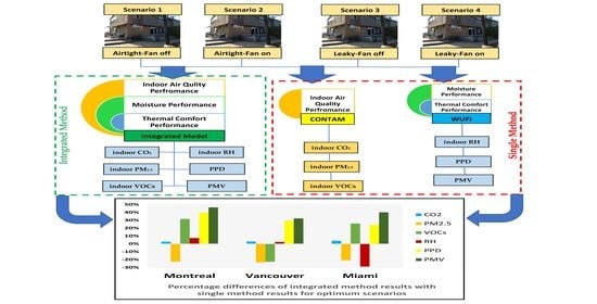
• Scenario 4 resulted in the optimal scenario for the indoor CO₂ performance in both the CONTAM model and the integrated model methods in Montreal and Vancouver. The integrated model calculates the indoor CO₂ performance for Scenario 4 in Montreal and Vancouver by differences of 2.80% and 3.02%, respectively, more than the CONTAM model. The reason for this difference is because in the CONTAM model method, the effective leakage area of 0.3 m² and exhaust fan airflow of 24 L/s are defined by the users as airflows input data. In contrast, the airflows in the integrated model method are corrected by the co-simulation mechanism for CONTAM–WUFI.
• To calculate indoor CO₂ performance in Miami, the results of Scenario 4, the optimal scenario using the integrated model method, are 3.98% different from the results of Scenario 2, the optimal scenario using the CONTAM model method. The reason for this difference is that the calculation of indoor CO₂ performance in Scenario 2 is defined by the user based on the effective leakage area of 0.04 m² and exhaust fan airflow of 24 L/s. The integrated model method in Scenario 4 calculates indoor CO₂ performance based on the corrected airflows using the co-simulation mechanism of CONTAM-WUFI.
• In calculating the indoor PM_2.5 performance, the results of Scenario 2, the optimal scenario by the integrated model method, are −22.65% different from the CONTAM model method. The reason for this difference is that in the CONTAM model method, effective leakage area of 0.04 m² and exhaust fan airflow of 24 L/s are defined as input airflows data by the user. Thus, in the integrated model method, with the help of the co-simulation mechanism of CONTAM–WUFI, the airflows values have been corrected.
• Scenarios 2 and 4 are predicted for both Vancouver and Miami in the optimal level of indoor PM_2.5 performance. The indoor PM_2.5 performance values calculated for these scenarios by the integrated model method are −23.4% and −20.95% different from the CONTAM model method for Vancouver and Miami, respectively. The reason for this difference is that in the CONTAM model method, the effective leakage areas of 0.04 m² and 0.3 m² and exhaust fan airflow rate of 24 L/s for Scenarios 2 and 4, respectively, are defined as input data airflows by the user. In contrast, the corrected airflows variables have been used by the integrated model method based on the co-simulation mechanism for CONTAM–WUFI.
• The values of the indoor VOCs performance for Scenario 4, the optimal scenario by the integrated model method, are 31.54% and −22.70% different from the CONTAM model method for Montreal and Vancouver, respectively. The reason for this difference is that in the CONTAM model method, the effective leakage area of 0.3 m² and exhaust fan airflow of 24 L/s are defined as airflows input data by the user. In the integrated model, the airflows variables are corrected by the co-simulation mechanism of CONTAM–WUFI.
• To calculate the indoor VOCs performance in Miami, the results of Scenario 2, the optimal scenario through the integrated model method, are 25.86% different from Scenario 4, the optimal scenario through the CONTAM model method. The reason for this difference is that the effective leakage area of 0.3 (m²) and exhaust fan airflow of 24 L/s for Scenario 4 are defined by the user as the input airflows data in the CONTAM model method. As in the integrated model method in Scenario 2, the corrected airflows data is used by the co-simulation mechanism of CONTAM–WUFI.
• In Montreal, for the calculation of the indoor relative humidity (RH) performance, the results of Scenario 3, the optimal scenario through the integrated model method, are 7.39% different from the results of Scenario 4, the optimal scenario based on the WUFI model method. Therefore, the reason for this difference is that in the WUFI model method, infiltration of 3.2 h⁻¹ and mechanical ventilation of 0.3 h⁻¹ for Scenario 4 are defined as airflows input data by the user. In addition, in the integrated model method for Scenario 3, corrected airflows are used by the co-simulation mechanism of CONTAM–WUFI.
• The results of Scenario 4, the optimal scenario in calculating indoor relative humidity (RH) performance through the integrated model method, are 2.55% and −28.8% different from the WUFI model method results for Vancouver and Miami, respectively. The reason for this difference is that the infiltration of 3.2 h⁻¹ and mechanical ventilation of 0.3 h⁻¹ are defined by the user as the input airflows data in the WUFI model method. In the integrated model method, the airflows data is corrected by the co-simulation mechanism of CONTAM–WUFI.
• In calculating the indoor percentage of dissatisfied (PPD) performance, the results of Scenario 1, the optimal scenario through the integrated model method, resulted in a 39.58, 29.39, and 23.99% difference in Montreal, Vancouver, and Miami, respectively, from the WUFI model method. The reason for this difference is that the infiltration of 0.4 h⁻¹ is defined as the input airflow data by the user in the WUFI model method. In contrast, in the integrated model method, air flow data corrected by the co-simulation mechanism of CONTAM–WUFI are used.
• In calculating the indoor predicted mean vote (PMV) performance, Scenario 1, the optimal scenario through the integrated model method, resulted in a 52.98, 32.41, and 40.18% difference in Montreal, Vancouver, and Miami, respectively, from the WUFI model method. The reason for this difference is that the infiltration of 0.4 h⁻¹ is defined as airflow input data by the user in the WUFI model method. However, the airflow data is corrected through the co-simulation mechanism of CONTAM–WUFI in the integrated model method.

5. Conclusions

In this research study, an integrated model was developed to predict the performances of indoor air quality, moisture, and thermal comfort. In this model, the three balances of heat, moisture, and contaminate flows are simultaneously coupled. The exchange of the airflow rate parameter between CONTAM and WUFI, using a coupling method for developing the integrated model, made it possible to control and modify this parameter and the simulation results based on ASHRAE Standard 62.1, 160, and 55 levels. With the integrated model, a modified airflow rate can be designed for buildings with the high performances of indoor air quality, moisture, and thermal comfort conditions according to ASHRAE Standard criteria.

To evaluate the integrated model in comparison with single models of CONTAM and WUFI, simulated indoor CO₂, PM_2.5, and VOCs concentrations, as well as indoor air quality measures, indoor relative humidity (RH) as moisture measures, percentage of dissatisfied (PPD), and predicted mean vote (PMV) as thermal comfort measures were provided in this study. The results of indoor CO₂, PM_2.5, and VOCs simulated by CONTAM were compared with the integrated model, and the results of indoor relative humidity (RH), percentage of dissatisfied (PPD), and predicted mean vote (PMV) by WUFI were compared with the integrated model, as well.

As per the differences between the results of the single models and the present integrated model, it can be deduced that when the integrated model method replaces the single models’ methods, the airflows data corrected by the CONTAM–WUFI co-simulation mechanism will replace with the airflow input data assumed by the user. Therefore, as these airflow data in the integrated model are corrected based on the capabilities of the coupled CONTAM–WUFI sub-models, it can accurately predict the results of the calculated indoor air quality, thermal comfort, and moisture performance for optimum scenarios for buildings subjected to various climatic conditions.

Considering that the accuracy of the integrated model was verified by the paired sample t-test method, it can be concluded that the results of the integrated model can be used as a benchmark in predicting the performances of indoor air quality, moisture, and thermal comfort compared to other single models. Therefore, any differences between the results obtained with the present integrated model and those obtained with the single models (i.e., CONTAM and WUFI) suggest that the integrated model method can be a reliable alternative to the single model method for accurately assessing the indoor air quality, moisture, and thermal comfort performances for one-story, two-story, and three-story buildings when they are subjected to various climatic conditions. Last but not least, the EnergyPlus model was recently coupled with the present integrated model to simultaneously assess the overall performance (i.e., energy, indoor air quality, and moisture with thermal comfort performances) of the same three-story house considered in this study when it was subjected to the climatic conditions of Montreal, Vancouver, and Miami [42].

References

1. Zhang, F.; de Dear, R.; Hancock, P. Effects of moderate thermal environments on cognitive performance: A multidisciplinary review. Appl. Energy 2019, 236, 760–777. [Google Scholar] [CrossRef]
2. Heibati, S.M.; Atabi, F.; Khalajiassadi, M.; Emamzadeh, A. Integrated dynamic modeling for energy optimization in the building: Part 1: The development of the model. J. Build. Phys. 2013, 37, 28–54. [Google Scholar] [CrossRef]
3. Heibati, S.M.; Atabi, F. Integrated dynamic modeling for energy optimization in the building: Part 2: An application of the model to analysis of XYZ building. J. Build. Phys. 2013, 37, 153–169. [Google Scholar] [CrossRef]
4. Rabani, M.; Bayera Madessa, H.; Nord, N. Building Retrofitting through Coupling of Building Energy Simulation-Optimization Tool with CFD and Daylight Programs. Energies 2021, 14, 2180. [Google Scholar] [CrossRef]
5. Fanger, P.O. Thermal Comfort. Analysis and Applications in Environmental Engineering. In Thermal Comfort. Analysis and Applications in Environmental Engineering. 1970. Available online: https://www.cabdirect.org/?target=%2fcabdirect%2fabstract%2f19722700268 (accessed on 10 June 2021).
6. ASHRAE. Thermal Environmental Conditions for Human Occupancy ANSI/ASHRAE Standard 55; ASHRAE: Atlanta, GA, USA, 2017. [Google Scholar]
7. Schweiker, M. comf: An R Package for Thermal Comfort Studies. R. J. 2016, 8, 341. [Google Scholar] [CrossRef] [Green Version]
8. Tartarini, F.; Schiavon, S. pythermalcomfort: A Python package for thermal comfort research. SoftwareX 2020, 12, 100578. [Google Scholar] [CrossRef]
9. Schiavon, S.; Hoyt, T.; Piccioli, A. (Eds.) Web Application for Thermal Comfort Visualization and Calculation According to ASHRAE Standard 55. Building Simulation. pp. 321–334. Available online: https://link.springer.com/article/10.1007/s12273-013-0162-3 (accessed on 10 June 2021).
10. Chen, Q. Ventilation performance prediction for buildings: A method overview and recent applications. Build. Environ. 2009, 44, 848–858. [Google Scholar] [CrossRef]
11. Wang, L.L.; Chen, Q. Evaluation of some assumptions used in multizone airflow network models. Build. Environ. 2008, 43, 1671–1677. [Google Scholar] [CrossRef]
12. Wang, L.; Wong, N.H. Coupled simulations for naturally ventilated residential buildings. Autom. Constr. 2008, 17, 386–398. [Google Scholar] [CrossRef]
13. Gao, N.; Zhang, H.; Niu, J. Investigating indoor air quality and thermal comfort using a numerical thermal manikin. Indoor Built Environ. 2007, 16, 7–17. [Google Scholar] [CrossRef]
14. Chang, S.J.; Wi, S.; Kang, S.G.; Kim, S. Moisture risk assessment of cross-laminated timber walls: Perspectives on climate conditions and water vapor resistance performance of building materials. Build. Environ. 2020, 168, 106502. [Google Scholar] [CrossRef]
15. Künzel, H.M. Simultaneous Heat and Moisture Transport in Building Components. One-and Two-Dimensional Calculation Using Simple Parameters; IRB-Verlag Stuttgart: Stuttgart, Germany, 1995; p. 65. [Google Scholar]
16. Details: Physics-Wufiwiki. Available online: https://www.wufi-wiki.com/mediawiki/index.php/Details:Physics (accessed on 15 June 2021).
17. Ibrahim, M.; Sayegh, H.; Bianco, L.; Wurtz, E. Hygrothermal performance of novel internal and external super-insulating systems: In-situ experimental study and 1D/2D numerical modeling. Appl. Therm. Eng. 2019, 150, 1306–1327. [Google Scholar] [CrossRef]
18. Mundt-Petersen, S.O.; Harderup, L.-E. Predicting hygrothermal performance in cold roofs using a 1D transient heat and moisture calculation tool. Build. Environ. 2015, 90, 215–231. [Google Scholar] [CrossRef]
19. Le, A.D.T.; Zhang, J.S.; Liu, Z.; Samri, D.; Langlet, T. Modeling the similarity and the potential of toluene and moisture buffering capacities of hemp concrete on IAQ and thermal comfort. Build. Environ. 2020, 188, 107455. [Google Scholar]
20. Zu, K.; Qin, M.; Rode, C.; Libralato, M. Development of a moisture buffer value model (MBM) for indoor moisture prediction. Appl. Therm. Eng. 2020, 171, 115096. [Google Scholar] [CrossRef]
21. Hunter-Sellars, E.; Tee, J.; Parkin, I.P.; Williams, D.R. Adsorption of volatile organic compounds by industrial porous materials: Impact of relative humidity. Microporous Mesoporous Mater. 2020, 298, 110090. [Google Scholar] [CrossRef]
22. Promis, G.; Dutra, L.F.; Douzane, O.; Le, A.T.; Langlet, T. Temperature-dependent sorption models for mass transfer throughout bio-based building materials. Constr. Build. Mater. 2019, 197, 513–525. [Google Scholar] [CrossRef]
23. Rode, C.; Grunewald, J.; Liu, Z.; Qin, M.; Zhang, J. Models for Residential Indoor Pollution Loads Due to Material Emissions under Dynamic Temperature and Humidity Conditions. In Proceedings of the E3S Web of Conferences; p. 11002. Available online: https://www.e3s-conferences.org/articles/e3sconf/abs/2020/32/e3sconf_nsb2020_11002/e3sconf_nsb2020_11002.html (accessed on 10 July 2021).
24. Sowa, J.; Mijakowski, M. Humidity-Sensitive, Demand-Controlled Ventilation Applied to Multiunit Residential Building—Performance and Energy Consumption in Dfb Continental Climate. Energies 2020, 13, 6669. [Google Scholar] [CrossRef]
25. Moschetti, R.; Carlucci, S. The impact of design ventilation rates on the indoor air quality in residential buildings: An Italian case study. Indoor Built Environ. 2017, 26, 1397–1419. [Google Scholar] [CrossRef]
26. Dols, W.S.; Emmerich, S.J.; Polidoro, B.J. Coupling the Multizone Airflow and Contaminant Transport Software CONTAM with EnergyPlus Using Co-Simulation. Building Simulation. pp. 469–479. Available online: https://link.springer.com/content/pdf/10.1007/s12273-016-0279-2.pdf (accessed on 10 July 2021).
27. Moujalled, B.; Aït Ouméziane, Y.; Moissette, S.; Bart, M.; Lanos, C.; Samri, D. Experimental and numerical evaluation of the hygrothermal performance of a hemp lime concrete building: A long term case study. Build. Environ. 2018, 136, 11–27. [Google Scholar] [CrossRef]
28. Chang, S.J.; Kang, Y.; Wi, S.; Jeong, S.-G.; Kim, S. Hygrothermal performance improvement of the Korean wood frame walls using macro-packed phase change materials (MPPCM). Appl. Therm. Eng. 2017, 114, 457–465. [Google Scholar] [CrossRef]
29. Fedorik, F.; Alitalo, S.; Savolainen, J.-P.; Räinä, I.; Illikainen, K. Analysis of hygrothermal performance of low-energy house in Nordic climate. J. Build. Phys. 2021. [Google Scholar] [CrossRef]
30. Heibati, S.; Maref, W.; Saber, H.H. Assessing the Energy and Indoor Air Quality Performance for a Three-Story Building Using an Integrated Model, Part One: The Need for Integration. Energies 2019, 12, 4775. [Google Scholar] [CrossRef] [Green Version]
31. CONTAM 3.2. National Institute of Standards and Technology Engineering Laboratory: USA, 2016; Ver. 3.2.0.2. Available online: https://www.nist.gov/el/energy-and-environment-division-73200/nist-multizone-modeling/software/contam/download (accessed on 11 July 2021).
32. WUFI® Plus. Thermal, Energy and Moisture Simulation of Building, Ver.3.2.0.1 ed.; Fraunhofer Institute for Building Physics: Stuttgart, Germany, 2021; Available online: https://wufi.de/en/webshop/ (accessed on 12 July 2021).
33. Heibati, S.; Maref, W.; Saber, H.H. Developing a model for predicting optimum daily tilt angle of a PV solar system at different geometric, physical and dynamic parameters. Adv. Build. Energy Res. 2019, 179–198. [Google Scholar] [CrossRef]
34. Mckeen, P.; Liao, Z. (Eds.) The Influence of Airtightness on Contaminant Spread in MURBs in Cold Climates. Building Simulation; Springer: Berlin/Heidelberg, Germany, 2021. [Google Scholar]
35. Dols, W.S.; Dols, W.S.; Polidoro, B.J. CONTAM User Guide and Program Documentation: Version 3.2. 2015. Available online: https://nvlpubs.nist.gov/nistpubs/TechnicalNotes/NIST.TN.1887.pdf (accessed on 15 July 2021).
36. Sherman, M.H.; Dickerhoff, D.J. Air-tightness of US dwellings. Trans. Am. Soc. Heat. Refrig. Air Cond. Eng. 1998, 104, 1359–1367. [Google Scholar]
37. Chan, W.R.; Price, P.N.; Sohn, M.D.; Gadgil, A.J. Analysis of US Residential Air Leakage Database; Lawrence Berkeley National Laboratory. 2003. Available online: https://escholarship.org/content/qt6pk6r4gs/qt6pk6r4gs.pdf (accessed on 17 June 2021).
38. EnergyPlus. EnergyPlus Documentation, Engineering Reference, The Reference to EnergyPlus Calculations 2015. Available online: https://energyplus.net/sites/default/files/pdfs_v8.3.0/EngineeringReference.pdf (accessed on 20 June 2021).
39. ASHRAE. Fundamentals Handbook. American Society of Heating, Refrigerating, and Air-Conditioning Engineers. 2017. Available online: https://www.ashrae.org/advertising/handbook-advertising/fundamentals (accessed on 25 June 2021).
40. Antretter, F.; Künzel, H.; Winkler, M.; Pazold, M.; Radon, J.; Kokolsky, C.; Stadler, S. WUFI® Plus, Fundamentals; Fraunhofer Institute for Building Physics: Germany, 2018; Available online: https://wufi.de/en/software/wufi-plus/#:~:text=WUFI%20%C2%AE%20Plus%20is%20the%20most%20complete%20heat,for%20addressing%20comfort%20and%20energy%20consumption%20in%20buildings (accessed on 22 June 2021).
41. Dols, W.S. A tool for modeling airflow & contaminant transport. Ashrae J. 2001, 43, 35–43. [Google Scholar]
42. Heibati, S.; Maref, W.; Saber, H.H. Assessing the Energy, Indoor Air Quality and Moisture Performance for a Three-Story Building Using an Integrated Model, Part Three: Development of Integrated Model and Applications. Energies 2021. submitted. [Google Scholar] [CrossRef]
43. HVAC Sizing. Available online: https://michaelbluejay.com/electricity/hvac-sizing.html (accessed on 27 January 2021).
44. ASHRAE. Energy Standard for Buildings Except Low-Rise Residential Buildings (I-P Edition); ANSI/ASHRAE/IES Standard 90.1; ASHRAE: Atlanta, GA, USA, 2019. [Google Scholar]
45. EnergyPlus. Weather Data Sources; U.S. Department of Energy’s (DOE) Building Technologies Office (BTO), and National Renewable Energy Laboratory (NREL): 2020. Available online: https://energyplus.net/weather (accessed on 26 June 2020).
46. CONTAM Utilities—CONTAM Weather File Creator, Version: 1.1; National Institute of Standards and Technology (NIST): 2014. Available online: https://www.nist.gov/el/energy-and-environment-division-73200/nist-multizone-modeling/software/contam-weather-file#:~:text=You%20can%20use%20the%20CONTAM%20Weather%20File%20Creator,Energy%20Plus%20weather%20files%20%28EPW%29%20to%20WTH%20files (accessed on 29 June 2021).
47. Haghighat, F.; Donnini, G.; D’Addario, R. Relationship between occupant discomfort as perceived and as measured objectively. Indoor Environ. 1992, 1, 112–118. [Google Scholar]
48. Emmerich, S.J.; Emmerich, S.J.; Gupte, A.; Howard-Reed, C. Modeling the IAQ Impact of HHI Interventions in Inner-City Housing; US Department of Commerce, National Institute of Standards and Technology: 2005. Available online: https://nvlpubs.nist.gov/nistpubs/Legacy/IR/nistir7212.pdf (accessed on 30 June 2021).
49. Canada, E.C.C. Canadian Environmental Sustainability Indicators Air Quality. 2018. Available online: https://www.canada.ca/content/dam/eccc/documents/pdf/cesindicators/air-quality/air-quality-en.pdf (accessed on 1 July 2021).
50. Division of Air Resource Management, FDoEP. 2019 Design Values for Fine Particulate Matter, PM2.5. Available online: https://floridadep.gov/sites/default/files/2019-PM2.5%20Design%20Values-Update.pdf (accessed on 3 July 2021).
51. Wallace, L.A.; Emmerich, S.J.; Howard-Reed, C. Source strengths of ultrafine and fine particles due to cooking with a gas stove. Environ. Sci. Technol. 2004, 38, 2304–2311. [Google Scholar] [CrossRef]
52. Howard-Reed, C.; Wallace, L.A.; Emmerich, S.J. Effect of ventilation systems and air filters on decay rates of particles produced by indoor sources in an occupied townhouse. Atmos. Environ. 2003, 37, 5295–5306. [Google Scholar] [CrossRef]
53. Ho, D.X.; Kim, K.-H.; Ryeul Sohn, J.; Hee Oh, Y.; Ahn, J.-W. Emission rates of volatile organic compounds released from newly produced household furniture products using a large-scale chamber testing method. Sci. World J. 2011, 11, 1597–1622. [Google Scholar] [CrossRef] [PubMed] [Green Version]
54. Craig, D.; Richard, S.; Gniffin, B. Finding System-Required Airflow. Available online: https://www.contractingbusiness.com/archive/article/20863033/finding-systemrequired-airflow (accessed on 27 January 2021).
55. Montreal, Quebec Climate & Temperature. Available online: http://www.montreal.climatemps.com/index.php (accessed on 5 July 2020).
56. Miami, Florida Climate & Temperature. Available online: http://www.miami.climatemps.com/index.php (accessed on 10 June 2020).
57. Vancouver, British Columbia Climate & Temperature. Available online: http://www.vancouver.climatemps.com/index.php (accessed on 20 April 2020).
58. IBM SPSS Statistics, 22.0 ed.; Armonk, NY, USA. 2021. Available online: https://www-01.ibm.com/common/ssi/ShowDoc.wss?docURL=/common/ssi/rep_ca/9/897/ENUS213-309/index.html&request_locale=en (accessed on 20 July 2021).
59. Zhu, Y. Applying computer-based simulation to energy auditing: A case study. Energy Build. 2006, 38, 421–428. [Google Scholar] [CrossRef]
60. ASHRAE. Ventilation for Acceptable Indoor Air Quality; ANSI/ASHRAE Standard 62.1; ASHRAE: Atlanta, GA, USA, 2019. [Google Scholar]
61. ASHRAE. Criteria for Moisture-Control Design Analysis in Buildings; ANSI/ASHRAE Standard 160; ASHRAE: Atlanta, GA, USA, 2016. [Google Scholar]
Figure 1. Co-simulation mechanism for CONTAM and WUFI. Abbreviations: ACH: air change rate; PRJ: project file; XLSX: Excel Microsoft Office open XML format spreadsheet file (XML: extensible markup language); ELA: effective leakage area; CONTAM: contaminant transport analysis; IDF: input data file; and WPS: WUFI plugin in SketchUp file.
Energies 14 04915 g001
Figure 2. Coupling method between CONTAM and WUFI equations.
Energies 14 04915 g002
Figure 3. Results of CONTAM for the IAQ performance based on the comparison of the indoor CO2 percentage difference on the acceptable level of ASHRAE Standard 62.1 for Montreal, Vancouver, and Miami.
Energies 14 04915 g003
Figure 4. Results of CONTAM for the IAQ performance based on the comparison of the indoor PM2.5 percentage difference on the acceptable level of ASHRAE Standard 62.1 for Montreal, Vancouver, and Miami.
Energies 14 04915 g004
Figure 5. Results of CONTAM for the IAQ performance based on the comparison of the indoor VOCs percentage difference on the acceptable level of ASHRAE Standard 62.1 for Montreal, Vancouver, and Miami.
Energies 14 04915 g005
Figure 6. Results of WUFI for the moisture performance based on the comparison of the indoor relative humidity (RH) on the acceptable level of ASHRAE Standard 160 for Montreal, Vancouver, and Miami.
Energies 14 04915 g006
Figure 7. Results of WUFI for the thermal comfort performance based on the comparison of the predicted percentage of dissatisfied (PPD) on the acceptable level of ASHRAE Standard 55 for Montreal, Vancouver, and Miami.
Energies 14 04915 g007
Figure 8. Results of WUFI for the thermal comfort performance based on the comparison of the predicted mean vote (PMV) on the acceptable level of ASHRAE Standard 55 for Montreal, Vancouver, and Miami.
Energies 14 04915 g008
Figure 9. Results of the integrated model for IAQ performance based on the comparison of the indoor CO2 percentage difference on the acceptable level of ASHRAE Standard 62.1 for Montreal, Vancouver, and Miami.
Energies 14 04915 g009
Figure 10. Results of the integrated model for IAQ performance based on the comparison of the indoor PM2.5 percentage difference on the acceptable level of ASHRAE Standard 62.1 for Montreal, Vancouver, and Miami.
Energies 14 04915 g010
Figure 11. Results of the integrated model for IAQ performance based on the comparison of the indoor VOCs percentage difference on the acceptable level of ASHRAE Standard 62.1 for Montreal, Vancouver, and Miami.
Energies 14 04915 g011
Figure 12. Results of the integrated model for moisture performance based on the comparison of the indoor relative humidity (RH) on the acceptable level of ASHRAE Standard 160 for Montreal, Vancouver, and Miami.
Energies 14 04915 g012
Figure 13. Results of the integrated model for thermal comfort performance based on the comparison of the predicted percentage of dissatisfied (PPD) on the acceptable level of ASHRAE Standard 55 for Montreal, Vancouver, and Miami.
Energies 14 04915 g013
Figure 14. Results of the integrated model for thermal comfort performance based on the comparison of the predicted mean vote (PMV) on the acceptable level of ASHRAE Standard 55 for Montreal, Vancouver, and Miami.
Energies 14 04915 g014