A Novel Automatic Method for the Urban Canyon Parametrization Needed by Turbulence Numerical Simulations for Wind Energy Potential Assessment

Abstract

The energy transition to more sustainable forms is currently ongoing worldwide, because of the environmental impacts produced by the non-renewable energy sources employed in the last decades. Among the main alternatives, wind plays a key role and, nowadays, innovative instruments, such as small-scale turbines allow for installation of wind turbines in urban areas. Their energy potential assessment requires high-accuracy simulations of the turbulent flows in the urban canopy layer, which, in turn, require detailed information about the geometrical properties of the basic element to classify urban surfaces, i.e., the urban canyon, often not available. In this work, we propose a novel automatic method, based on Voronoi graph, to univocally identify urban canyons and to extract their geometrical parameters from online available GIS (Geographic Information System) data, and test it on four European cities that differ in size, story and location. Results show the capability of the method to identify the single urban canyon and to properly extract its geometrical parameters, which tend to assume similar values for the largest cities. Moreover, we first attempt to propose and test some curves to generally describe the data probability distribution, which may be useful for turbulence simulations for urban wind energy assessment and planning. The best results are found for the canyon aspect ratio.

1. Introduction

Recently, the evidence of the climate changes, with the exponentially increasing carbon dioxide concentration in atmosphere and the consequent global warming, has raised awareness among governments and international institutions of the importance of rapidly reaching climatic neutrality by completing the energetic transition from fossil fuels to renewable energy sources. Therefore, renewable energies are becoming one of the most important research fields of our age. Among renewable energy sources, wind is currently playing a key role [1,2] since the wind turbines have proven their effectiveness, their efficiency is continuously increasing, and related technology is under constant enhancement [3,4,5,6,7], even looking to urban areas applications [8,9,10]. In the last years, the size of the wind turbines is continuously increasing because of the beneficial scale effects. The use of these devices is limited to farms located offshore or in sparsely populated rural areas. Therefore, the demand for distributed production is met with the help of small-scale turbines installed over high buildings (see, e.g., [11,12,13,14,15]). Recent results show the significant potential of the small-scale wind power generation [12,15,16,17]. Moreover, the implementation of distributed generator (smart-) grids over the urban area would have important advantages, such as low transmission losses and natural integration with the energy communities.

Small-scale turbines for wind energy conversion in urban environments are usually divided into two principal groups: horizontal axis wind turbines (HAWTs) and vertical axis wind turbines (VAWTs). According to the literature [18,19], VAWTs are the best choice for wind energy exploitation in urban environment, due to their capability to handle rapid wind direction changes and to their low noise emission compared to other turbines. Roof-mounted wind turbines demonstrated their effectiveness in providing decentralized renewable energy, and recent literature demonstrates that they can be successfully applicable to small size and low rise residential buildings, too [18]. However, technical aspects must be supported by economics evaluations: financial feasibility depends on several variables, such as resource potential, capital and operational costs, electricity prices, etc. Even if small-scale urban turbines require less technical effort and smaller capital and operating costs, pre-installation impact assessment is necessary to evaluate the technical feasibility and the optimum location for new turbines installation. The correct assessment of the wind energy potential is crucial for subsequent evaluations and analyses [20,21], and often turbulence modelling over urban surfaces is required [22]. A number of studies (see the review in [13]) are focused on this topic, supporting diverse possible approaches, as analytical procedures, laboratory experiments, probabilistic methods and computational fluid dynamics (CFD) simulations.

Referring to the first approach, the well-known log-law can be employed for the estimation of the mean wind speed vertical profile, valid for atmospheric boundary layer under neutrally-stable conditions [23], considering in-situ observations carried out above the urban canopy during a statistically significant period. However, this procedure is not simple and some authors have proposed alternative approaches that permit to use wind measurements carried out in meteorological stations nearby the investigated location, considering the anemological effects due to the presence of buildings and vegetation [20]. In addition, laboratory-scale experiments can be used to estimate the wind conversion potential [24]. Probabilistic methods are mainly based on specific studies [25], involving Weibull and Rayleigh probabilistic distributions for wind speed, with parameters depending on the site anemometric properties and on the height of the building on which turbines are intended to be installed.

Furthermore, the CFD methods are involved in simulating the turbulence for urban aerodynamic and microclimate modelling, thanks to their increased ability to reproduce the urban canopy. When the assessment method belongs to this last category, it is necessary to have information about the inlet velocity profile, which is fundamental for defining the boundary conditions of the model. In this case, authors suggest the usage of specific equations and schematizations [26]. Alternatively, or in combination, mesoscale modelling, coupled with urban canopy models (UCMs), is currently applied to provide boundary conditions for CFD simulations [27] as they can be used to estimate wind direction and intensity over urban surfaces [20]. Nevertheless, the determination of urban surface properties, in terms of building geometry (i.e., the urban morphology) and materials, is necessary for the accuracy of simulations [28]. This set of information is often defined as the urban canyon parameters (UCP) [29,30].

To give a response to the above-described needs, the aerodynamic model user community started development of the World Urban Database and Access Portal Tools (WUDAPT) project. The main purpose of WUDAPT is the collection of information about cities useful for climate, weather, and environment studies and for urban planning, including urban texture morphology and building construction materials. Information is shared and made available through the WUDAPT website [28]. The information is organized in layers with different levels of detail, in which data can be manipulated following specific procedures and protocols. In particular, level L0, i.e., the lowest data level, categorizes surfaces in the so-called local climate zones (LCZs) [31]; L1 describes building characteristics with high resolution, and L2 provides complete information about all urban elements, as building footprints and heights. L0 contains information about the thermal-related features, which have a clear role in the anthropogenic heat and, consequently, in the urban heat island (UHI) phenomenon. This information is usually obtained using Landsat data, image processing and local urban experts’ knowledge. The latter is crucial in defining and using the so-called training areas (TAs): the user identifies a TA in a LCZ of a particular type to compare its morphological characteristics with the ones of the rest of the city, parted in sub-zones, and consequently categorize them (i.e., assign a LCZ) on the basis of a criterion of similarity. After this process, a random forest (RF) classification algorithm, implemented in the SAGA GIS software [32], is used to classify Landsat scenes into LCZ maps. Even if L0 outputs are largely utilised, a method for acquiring, managing, and using higher level data is currently in progress.

Several activities are ongoing to improve WUDAPT and its products, developing detailed urban databases in which L1 and L2 data have higher spatial resolution and contain more variables. One of the most useful tools is the LiDAR (light detection and ranging), used to estimate aerodynamic parameters by remotely acquiring information about building characteristics [21,33]. In addition, advanced satellite data and processing algorithms can provide specific geometrical urban parameters [34]. According to their results, Google Earth high-resolution imagery (0.61 m) can be used to derive high-level UCPs and enhance model performance: this case study in Guangzhou demonstrated an improvement in modelled wind speed estimation using detailed UCPs data. Other extensions are possible, e.g., determining 3D buildings models, when urban morphology data are not available, and analysing relevant parameters as building coverage ratio (BCR), building height (BH), building volume density (BVD), frontal area index (FAI), sky view factor (SVF) and roughness length (RL) as investigated in [35]. The latter study is carried out in the frame of WUDAPT to improve L1 and L2 datasets. Other strategies involve the use of Convolutional Neural Networks (CNNs) [36], for assigning LCZs categorical to a certain portion of urban texture, or involving high level elaborations as object-based image analysis, as in [37]. However, during the initial phases of the characterization, local expertise is needed to assign parameters values to TAs.

In the present study, we propose and test an automatic method for the determination of some UCPs. The automatic procedure presented hereafter is based on the determination of street canyons via a Voronoi diagram and has been tested on four real European cities, starting with Geographic Information Systems (GIS) data, available online, with Digital Elevation Model (DEM) information. The UCPs extracted in this way allow a non-ambiguous identification of the basic element (the urban canyon) and a detailed morphometric characterization of urban canopies in turbulence numerical simulation finalized to the wind energy assessment of small-scale turbines; but also, among the others, for thermometric analysis in urban zones (e.g., for the reduction of the urban heat island phenomenon and, consequently, for energy consumption optimization in buildings and cities). To our best knowledge, this is the first time an automatic procedure based on Voronoi diagram is employed to the unique identification of urban canyons on real cities and to extract the UCPs. Moreover, this can be useful for supporting local experts or citizens involved in this type of data collection [38]. Eventually, we do a first attempt to propose some laws to generally describe the distribution of the main UCPs.

The paper is organized as follows: in Section 2 the main investigated UCPs are described; in Section 3 the case study cities are introduced; in Section 4 the automatic method is described; and in Section 5 the main results are shown and discussed, and a representativity test on the proposed distributions for the UCPs is displayed.

2. Main Investigated Parameters

In the present work we focus on four principal parameters for canyon description: canyon aspect ratio (ARc), building aspect ratio (ARb), canyon length (L) and canyon length to height aspect ratio (LAR). Figure 1 summarizes the principal urban canyon descriptors, showing an example of urban canyon used for the parameters definition. The canopy elements defining the considered section of urban canyon are delimited by the blue rectangle in the planar view in Figure 1a. The length of the canyon is indicated with L and buildings’ widths on each canyon side with Wb1 and Wb2. In Figure 1b, showing a frontal view of a sample canyon, the canyon width (Wc) and the buildings’ heights (H1 and H2) are given.

More details about the assumptions carried out for the detection of the canyon and for its surroundings definition, for the choice of building walls extension, for the Wbs derivation and for the computation of Hs are given in Section 4 (Methods). Note that, in a realistic situation, the buildings’ widths (Wb1 and Wb2), the building heights’ (H1 and H2) and the canyon width (Wc) can assume different values along the canyon axis, so the mean values along the canyon length are hereafter considered. Additionally, we characterize the width and height of the building pertaining to the canyon by averaging the elements on both sides. Therefore, Wb and H are defined as follows:

$$Wb=\frac{1}{2} \left(Wb1+Wb2\right)$$

(1)

$$H=\frac{1}{2} \left(H1+H2\right)$$

(2)

and the three main parameters under study, beyond L which was yet defined, are:

$$ARc=\frac{Wc}{H}$$

(3)

$$ARb=\frac{Wb}{H}$$

(4)

$$LAR=\frac{L}{H}$$

(5)

3. Case Studies

The cities of Cagliari, Rome, Berlin, and London were chosen as case studies to test the proposed automatic UCP detection methodology (Figure 2).

These case studies were specifically chosen because of their mutual differences, with the purpose of considering various urban texture typologies and city configurations and, hence, ensure a good representativity. Cagliari is an old town, where the first settlements can be dated to the pre-historic age. A large part of edification and construction belong to the Medieval Period, and many characteristic architectural shapes are still present, embodied in the modern urban texture. Rome was founded, according to traditional knowledge, in 753 B.C. It is the third most populous European city, after Berlin and Madrid and includes an enormous variety of architectural styles. Berlin was probably founded around the XII century and developed in a completely different context with respect to the previous cities described, with comprehensible implications in its architectonical features. London’s first principal settlement was built up by Romans in 43 A.D., although some independent villages were present around the site. Surely, the Great Fire of London in 1666 contributed to an important re-drawing of the urban texture, adding differences and peculiarities.

For each city, a test area including the city centre and the surrounding districts have been chosen in order to include several different urban typologies, from both the architectural and historic point of view. In particular, Rome (1285 km² extension) and London (1572 km² extension) are represented by the largest sampling zones (159.85 and 94.47 km²), followed by Berlin (891 km² of city extension and 33.90 km² of sampling zone extension) and Cagliari (85.45 km² city extension and 3.52 km² sampling zone extension). Basic information on buildings’ heights and position for each case study are available thanks to the Copernicus project [39], with the exception of Cagliari, for which data is available thanks to local government initiative [40]. For morphological analyses, Digital Elevation Models (DEMs) were used (both Digital Terrain Models, DTMs, and Digital Surface Models, DSMs). In particular, for Rome, Berlin and London, the initial dataset was the one provided by the European Land Monitoring Service, through Copernicus project and web interface (https://land.copernicus.eu/local/urban-atlas/building-height-2012, accessed on 1 June 2021): the product is generated starting from IRS-P5 stereo images acquired as close as possible to the defined reference year (2012). Based on these stereo images, a digital surface model is generated. Afterwards a DTM is derived from the DSM with different filter algorithms and the assistance of Urban Atlas 2012 (the Copernicus project related to urban information derivation around Europe) datasets. The calculation of the normalized DSM is done by a simple subtraction of the DTM from the DSM. For Cagliari, instead, DEMs were available thanks to the local data acquisition and storage project “Sardegna Geoportale” (http://www.sardegnageoportale.it/areetematiche/modellidigitalidielevazione/, accessed on 2 June 2021). DTMs and DSMs were, in this case, LiDAR method based, accurately localized by means of Global Positioning System (GPS). For Cagliari elevation information, filtering was applied for building height determination, as well as for the other considered cities. As a conclusion, the employed building height data were already post-processed and validated by institutional providers, ensuring to avoid information errors caused by bad weather or not-optimal conditions for the reconnaissance flights.

4. Method

Geographic Information Systems (GISs) are useful tools for building data acquisition and processing. In this study, GISs have been largely employed for data treatment, starting from the manipulation of buildings’ heights information stored in DEMs [41].

The urban texture of many old European cities is irregular, different from the regular grid of perpendicular streets that characterizes many modern cities. A first idea to properly analyse urban textures is to use adaptative street graph-based grids. A previous study [42] showed that an adaptative grid can more realistically reproduce site specificities, providing an accurate quantitative representation of morphometric features such as λ_p (the building planar area index) and λ_f (the building frontal area index).

The first possible obstacle encountered during a street-graph urban partition is linked with the nature of the used data. For instance, available street-graph data (e.g., provided by Open Street Map, OSM [43]) include several elements classified as streets though they are not: e.g., train stations may be represented with multiple lines or large boulevards with more than one axis, and so are included more than once in the statistics. A supervised pre-processing of the street-graph data to resolve these incongruencies may be feasible on small study zones but it can be hardly used over large urban areas. Moreover, a street-graph method cannot provide an accurate street canyon subdivision, in particular regarding their length (L). In fact, urban data are not morphometric oriented, and vectorial information on streets may include a large amount of canyon non-representative elements (as double axis for large streets, city squares delimitation or street curves in crossroads) and, specifically referred to L computation, a single canyon cannot be straight and linear, thus deviating from the idealized definition of street canyon. On the other hand, it may not include other relevant information for the identification of street canyons, such as pedestrian street.

To overtake these issues, an automatic method, based on Voronoi polygons (VP), to obtain a non-arbitrary subdivision of urban texture into urban canyons, starting from available online databases, was developed. The basic idea is to create the Voronoi polygons around buildings in order to associate a specific VP to each building (hereinafter, VP around buildings will be indicated with VPb). Since every VPb thus created consists of a certain number of sides (determined by the planar partition, depending on both the number and position of other buildings, see below), it is possible to assume every VPb side as an urban canyon, and to establish the pertinent number of canyons around each building. In this way a quantitative analysis of the canyon geometrical features can be performed automatically, even on large urban areas. The VP were previously employed for other purposes, e.g., for morphometric analyses for urban climate studies [44], but also for urban planning (as method to divide the whole territory for census and population-related statistics determination [45]), for the detection of ventilation paths [46] and for the estimation of diurnal cycle of the surface energy balance fluxes [47]. In these cases, through VP, authors obtained a territorial partition, and their application was polygon-oriented, as every polygon was considered an element of the planar subdivision. In the present method, VP are a mean to obtain arcs and nodes of a graph and, consequently, to provide the first localization of each urban canyon. After non-supervised re-arrangements of this first localization, the method unequivocally identifies single urban canyons and then derives their UCPs, as better described below in the present section. In other words, to the best of the authors’ knowledge, this is the first time an automatic procedure based on Voronoi diagram is employed for the unambiguous identification of urban canyons in real cities and to extract their UCPs.

Usually, Voronoi polygons are defined around points [48], but generalizations have been conducted in recent decades [49]. By defining Voronoi polygons around buildings, it is possible to consider that every polygon can be interpreted as a line, and every line can be interpreted as a collection of points: so, VPb is the envelope of VP associated at each point. The idea can be so extended to lines and polygons and implemented even in a GIS software [50].

First, the raw GIS images, with every pixel containing the DEM information about the elevation, need to be preprocessed (see Figure 3). In the first step, the DEM is processed to have zero height values on the streets (following the procedure defined in [42]) and then the images are binarized, in order to separate the streets (zero-height pixels) from the buildings (non-zero height pixels). Then holes in the binary image of the buildings, usually internal courts, are filtered to facilitate the determination of the external border of buildings. It should be noted that internal courts are neglected only to facilitate this step of the procedure, but they are then taken into account in the following analysis of the building width. Moreover, a building adjustment is conducted by means of erosion techniques (to delete smaller elements attached to main buildings, non-contiguous or semi-contiguous) and image opening (to separate different buildings erroneously united, due to low resolution). Eventually, a statistical analysis on most frequent building volumes, allows for the definition of a minimum value for the building dimension, employed to remove the smallest elements, such as kiosks, which are not relevant for the street canyon definition.

Once the images have been preprocessed, they are ready to be elaborated with the proposed procedure. Figure 4a shows how buildings’ contours can be interpreted as a collection of points, corresponding to the corner of the buildings. These points are then tightened (i.e., the number of points on straight segments forming the contour is increased) to improve the accuracy of calculations, employing a function included in QGIS (Figure 4b). Figure 4c depicts the creation of VP around each point in the plane. Once VP are created, VP around points related to the same building can be merged together (Figure 4d) and the specific VPb (Figure 4e) can be defined. In fact, this union forms the planar area which is identified as the set of the points which are nearer to the considered building than to every other in the analysed urban texture. This geometrical criterion ensures the unique assignment of each point to a single building. To conduct the just described elaboration, v.voronoi function of GRASS GIS (https://grass.osgeo.org/grass79/manuals/v.voronoi.html, accessed on 10 June 2021) based on the “sweep line algorithm” was used. At this point, the border of the VP is identified as the street axes (Figure 4f).

In this way, a Voronoi graph (VG) composed by the street axis can be defined. Moreover, each side of two different VPbs can be defined as an arc and each node is the intersection between two or more arcs. Figure 5a shows an example of the VG obtained through the above-described procedure: each arc is depicted with a different colour, while the red points represent VG nodes. The only adjustment left to the user is the definition of a minimum length for canyons (10 m in the results shown below) to neglect too short traits, created by the planar partition depending on mutual distances between buildings. The decomposition of Voronoi tessellation to obtain the VG was executed by the “Polygons to Edges and Nodes” function of SAGA GIS. Once the VPbs are built, it is important to preserve for each arc information about the two polygons sharing that arc.

In this way, the arc between two nodes is identified as an urban canyon axis and every canyon can be univocally identified and so, quantitatively characterized. For each of the defined street canyon elements, cross streets (identified by a node) imply the canyon interruption. A street canyon is, consequently, a continuous line (i.e., an arc). Furthermore, the proposed method excludes ambiguities linked to city squares, as they are parted by Voronoi diagram as every other zone. Eventually, this procedure allows, among the others, to solve the problem of the double axis on the same street, as a consequence of the unique identification of a street as an arc of the Voronoi graph.

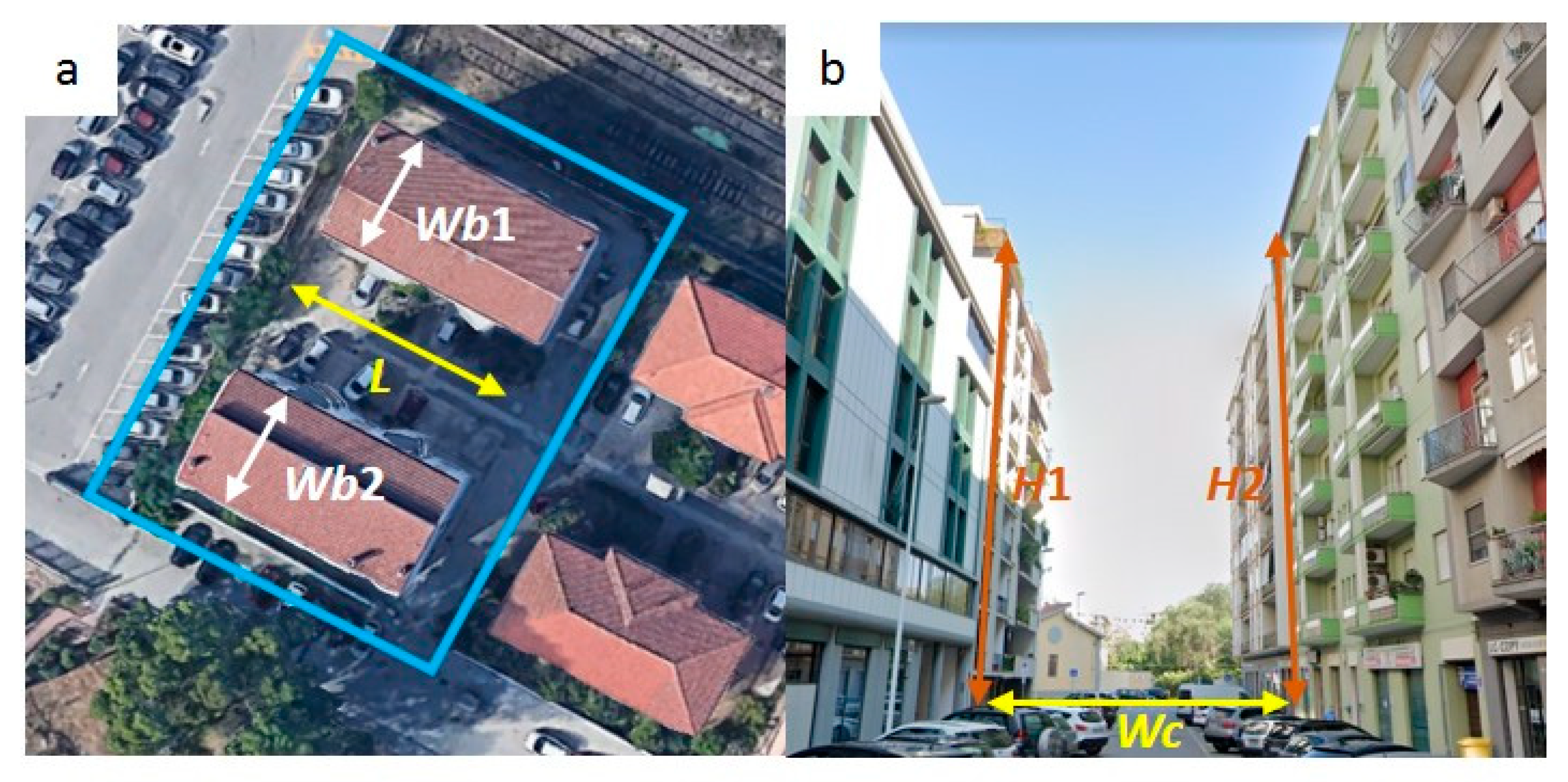
Figure 5b shows an example of this canyon characterization. Once pertinent nodes are identified, the arc is rectified in order to determine a unique direction perpendicular to the canyon axis (the continuous red line on Figure 5b), and the raster image is rotated in order to align the axis of the canyon along the columns of the data array (representing the height of the buildings or the streets). Then, the transversal sections are aligned along the data rows (dashed red lines). Then, the canyon length L is divided into a certain number of sections, $n_s$, separated by a distance $p_s$ (in the analysis shown in Section 5, the minimum distance of one pixel, allowing the maximum resolution, was employed). On each section, the width, $w{c}_i$, of the canyon at the i-th row of the raster image is defined as the distance between the closest two points belonging to the opposite buildings (the red points on Figure 5b). Wc is then computed as the average of all the $w{c}_i$ along the canyon axis. A similar procedure is then adopted to identify the far end of the buildings along the same section (green points on Figure 5b) and so the width Wb is the average of the $w{b}_i$. Each building section $w{b}_i$, consisting of $n{b}_i$ pixels, can have different heights, $h_{ij}$, so the average height of the building H is computed as the average of all the $h_{ij}$ belonging to the building. It is worth mentioning that an arc (i.e., a street canyon) is defined by two, and only two, buildings. Therefore, there is no ambiguity about the elements to consider during the UCPs computation. Equations (6)–(9) report a detailed description of how the main canyon cross-section parameters (Wb, Wc, H) are computed. $\overline{h_i}$ is the average building height value for the section i.

$$W_b=\frac{1}{n_s} {\displaystyle \sum }_{i=1}^{n_s}w{b}_i$$

(6)

$$W_c=\frac{1}{n_s} {\displaystyle \sum }_{i=1}^{n_s}w{c}_i$$

(7)

$$\overline{h_i}=\frac{1}{n{b}_i} {\displaystyle \sum }_{j=1}^{n{b}_i}{h}_{ij}$$

(8)

$$H=\frac{1}{n_s} {\displaystyle \sum }_{i=1}^{n_s}\overline{h_i}$$

(9)

To check the accuracy of the above proposed automatic method for the quantitative evaluation of UCPs, a test on different small areas of Cagliari was initially conducted. Several canyons with various characteristics were considered and UCP values for these were firstly manually determined, using simple measuring functions in QGIS and Google Earth. Then, the manually derived values were compared with the ones generated by the automatic method, showing a good accordance. Afterwards, we tested the automatic procedure in the other cities, to verify its suitability for different urban texture conformation and peculiarities. The capability of the procedure to properly identify the single canyons and to measure their characteristics was confirmed. Furthermore, we verified if the non-supervised method was able to resolve some particular cases deriving from the GIS street graph information, such as double street axis, roundabouts and squares, curved streets. Figure 6 shows that these cases are properly solved by the method.

In conclusion of the method description,

Table 1. Specifications on site characteristics, number of detected canyons, DEM resolution after pre-processing and computational time.

City	Extension (km2)	Detected Canyons (-)	DEM Resolution (Pixel Side Length) (m)	Computational Time (h)
Cagliari	3.52	6752	1	15.25
Rome	159.85	17,574	0.75	65.33
Berlin	33.90	6180	0.65	26.20
London	94.47	21,455	0.65	62.03

reports some specifications on site characteristics, number of detected canyons, DEM resolution after pre-processing and computational time. Extensions of the four case studies are quite different, but this is not the only parameter considered to evaluate necessary resources. In fact, depending on available computational power, any geographical extension may be analysed with this automatic method. There are no particular limitations on DEM resolution: the ones reported are those defined after a pre-processing phase. In fact, for Rome, Berlin and London, in Copernicus datasets (cited in Case Studies section) the original pixel side length was 10 m; some important pre-operations as geo-referencing and, even more, manipulations as image erosion and opening, require a higher pixel subdivision to work properly, even if height information in input does not actually change. Cagliari dataset is an exception since a DEM with 1 m sided pixels is available and downloadable through the local institution’s website cited above. It should be noted that the number of detected canyons is more related to the length of the canyon L (see Section 5.2) than to the city extension.

5. Results and Discussion

As reported in the Introduction, the demand for distributed renewable energy production from wind sources can also be met with the help of small-scale turbines installed over high buildings, and VAWTs are the best choice for wind energy exploitation in urban environment [1,2,3,4,5]. For wind energy potential assessment, numerical and laboratory simulations of urban boundary layer turbulence require a detailed description of geometric characteristics of the urban canopy in form of UCPs [16,17]. In this Section, the results obtained following the above-described unsupervised procedure for the determination of urban canyon geometrical parameters UCPs are summarized.

In the first Subsection, the probability distribution functions for each UCP and for the four test cases will be shown, as well as a first proposal of best-fit functions to summarize the data. In the second Subsection, a statistical analysis, based on Q-Q (Quantile-Quantile) plots, will be performed, to test the capability of the proposed fitting functions to represent the data.

5.1. Probability Density Functions and Proposed Distributions

Figure 7, Figure 8, Figure 9 and Figure 10 show the probability density functions (pdfs) for the four parameters investigated (i.e., ARc, ARb, L and LAR, respectively) and for the four case studies (i.e., the four test areas in the four European cities). Together with the single values, shown with cyan bars, for every city-parameter couple, the main descriptors of the distribution are reported, too. The average and median values are depicted by the magenta and the red lines, respectively, and their values are reported in the legend with the same colours. Moreover, the green line shows the maximum likelihood estimation best-fit distribution curve for the data, i.e., a Weibull distribution for ARc, ARb and LAR, and an exponential distribution for L. The most probable values of the data and of the fitting curve are reported in the legend in cyan and green, respectively. The equations for the distributions are:

$$f\left(x|a,b\right)=\frac{b}{a}{\left(\frac{x}{a}\right)}^{b-1}{e}^{-{\left(x/a\right)}^b}$$

(10)

for the Weibull distribution, and

$$f(x|\mathsf{\mu })=\frac{1}{\mathsf{\mu }} e^{-x/\mathsf{\mu }}$$

(11)

for the exponential distribution. The values of the parameters of Equations (6) and (7) for the four UCPs and the four test cases are reported in

Table 2. Parameters for the proposed distributions.

		Cagliari	Rome	Berlin	London
ARc	a	0.772	0.431	0.524	0.508
	b	1.312	1.119	1.261	1.229
ARb	a	0.894	1.042	1.161	1.108
	b	1.812	1.438	1.332	1.418
L	µ	34.904	59.573	105.033	58.337
LAR	a	3.903	5.618	7.534	6.959
	b	1.594	1.445	1.261	1.268

. For sake of clarity, for each UCP, only the most significative values are reported (i.e., those with very low probability, i.e., the extreme of the right tail in the pdfs, are truncated).

For wind energy potential assessment in urban areas, quantitative knowledge about UCPs and, more specifically, ARc values for a canyon area is required [16,17], even to conduct in-canyon motion analyses and conceptualization, as described below. Figure 7 shows that the distribution of ARc values has a similar trend for all cities, with an increase and a peak followed by a decrease. The most probable value is 0.15 for all the cities, apart from 0.25 for London. This corresponds to very narrow urban canyons, characterized by multiple vertical vortices with a diameter similar to the canyon width, which makes the ventilation at street level very difficult [51]. On the other hand, this corresponds to a skimming flow above the buildings, almost undisturbed, that favours the installation of small-scale turbines. As a matter of fact, if a wind turbine should be installed on a building at the end of a larger urban canyon (ARc larger than 1.5), i.e., under a wake interference or isolated roughness regime, the recirculation zone above this building would be larger and the efficiency of the energy conversion would be reduced. Furthermore, in the case of wake interference regime or isolated flow, the greater interaction between the vortical structures that develops within the canyons and the outer flow can slow down the external flow at the rooftops and canyon tops, reducing the energy efficiency of the turbines. The fitting curves show a maximum at 0.15 for Berlin, coinciding with the most probable value of the data, whilst the values of 0.06 for Rome and of 0.13 for London underestimate the respective most probable values. On the opposite, the peak of the fitting curve for Cagliari is at 0.26, with an overestimation of the actual value. So, the fitting curves correctly estimate the overall data behaviour, but are not always able to catch their most probable value. Regarding the mean value, Berlin (0.38), London (0.34) and Rome (0.29) show similar values, whilst Cagliari (0.57) has the largest value. This is due to the fact that Cagliari is the smallest city among the four, with a wider right tail (i.e., the large canyons have a higher probability than the other three cities). It is interesting to note that, employing these mean ARc values to classify the test cities into LCZ, they will all fall into LCZ5 (open midrise) or LCZ6 (open low-rise) classes, which both have a range for ARc of 0.3 ÷ 0.75. The same consideration can be drawn for the median, which has a larger value than the mean.

ARb values (Figure 8) show a trend similar to ARc, well described by the Weibull distribution. The most probable value for this parameter is 0.55 for all the cities, apart from Cagliari (0.65), i.e., the buildings tend to have a height, which is slightly less than twice the width (slender buildings). This configuration does not favor the installation of small-scale turbines, as slender buildings tend to increase the turbulence above the rooftops [52]. The maximum value of the fitting curve always underestimates the most probable value. Mean values are always in the range 0.69 (Cagliari)–0.78 (Berlin), while the median values are not far from 1.00 for all the cities, except for the smallest one, Cagliari, which has a median of 0.79. The higher value of Cagliari is attributable to the narrower distribution of ARb, since buildings in small cities tend to have a similar shape, whilst it is more probable to find wider buildings in the largest cities. The latter configuration favours the fluid reattachment on the building roof and, consequently, a more stable flow for the installation of wind turbines.

L and LAR, are relevant, among the others, as input for atmospheric turbulence models, such as the advanced street canyon module in the ADMS (atmospheric dispersion modelling system)-urban dispersion model (see, for instance [53,54]).

The values of L and its related statistical quantities are reported in Figure 9. A descending trend is identifiable and so, the behaviour differs from ARc and ARb. For this reason, L data were fitted with an exponential curve rather than a Weibull distribution. The most probable length is 25.00 m for the Italian cities (Cagliari and Rome), and 15.00 m for Berlin and London. Cagliari has the shortest right distribution tail, revealing the non-metropolitan nature of this city (i.e., that the probability of finding very long streets is lower), while Berlin has the longest one. In fact, Cagliari has the smallest values for the mean (27.00 m) and the median (34.90 m) values, while Berlin has the largest ones (76.00 m and 105.03 m for the mean and median, respectively). Rome and London show similar values (a mean of 45.00 m for Rome and 42.00 for London; a median of 59.97 m for Rome and 58.34 m for London).

The LAR data are reported in Figure 9. As for the other ARs, the trend that best approximates the real data is the Weibull one. Most probable values show the prevalence of short canyons (LAR is less than 3 for all the cities) and this is well predicted by the fitting curves, even if these always slightly overestimate the actual value (except for London, where the peak of the Weibull slightly underestimates the most probable value of the data). Mean and median values are under 7 for all selected cities (value usually employed for the long canyons), so they fall in the typical range of medium canyons [55].

The results highlight that, if on the one hand it seems to be feasible a generalization of the trends of the UCPs, on the other hand, the cruciality of a site-specific investigation is evident and an automatic method is fundamental for site-specific investigations.

5.2. Statistical Analysis of the Proposed Distributions

To test the representativity of the best-fit distributions introduced above, we conducted two analyses: one on the Q-Q plots and one on the main central moments for statistic samples of the four case studies.

To deepen the comparison between the pdf and the proposed best-fit curves, Figure 11, Figure 12, Figure 13 and Figure 14 report the Q-Q plots, following the same order used for the pdf figures. A Q-Q plot allows the comparison of two datasets by plotting their quantiles against each other. In particular, in the following plots, the actual data are on the Y-axis and the proposed best-fit curves are on the X-axis. Moreover, the bisector (perfect correspondence between actual data and best-fit curves) is drawn as a black straight line, as well as two red straight lines highlighting a tolerance interval. The values of the employed tolerances are reported in

Table 3. Cumulated density function at the reference point (i.e., the last point where data are still included in the tolerance interval) for the various UCPs.

City	Parameter	Tolerance	Reference Point on Q-Q-Plot	Cumulated Density Function Value at Reference Point
Cagliari	ARc	±0.2 (-)	2.5 (-)	98.77%
Rome			2.0 (-)	99.39%
Berlin			2.1 (-)	99.47%
London			1.7 (-)	98.29%
Cagliari	ARb	±0.3 (-)	2.1 (-)	97.31%
Rome			2.9 (-)	97.78%
Berlin			3.4 (-)	97.78%
London			3.0 (-)	97.43%
Cagliari	L	±20 m	60 m	92.70%
Rome			120 m	92.25%
Berlin			310 m	96.25%
London			190 m	97.78%
Cagliari	LAR	±1.2 (-)	10 (-)	97.93%
Rome			14 (-)	96.77%
Berlin			21 (-)	96.95%
London			17 (-)	94.70%

, as well as the cumulated density function value at the reference point (i.e., the last point where actual data are still included in the tolerance interval) for the various UCPs.

Figure 11 shows that the proposed Weibull distribution properly fits the ARc data for most of the interval, for Cagliari, Rome and Berlin, as the Q-Q data tend to follow the bisector, whilst London exhibits a slightly different behaviour. It should be noted that all the Q-Q data stay in the tolerance interval for more than the 98% (see Table 3). This means that the proposed Weibull distribution is able to describe the ARc data for the test cases with the exclusion of the right tail, which considers a minimum quantity of data. In Figure 12, the same analysis is carried out for ARb and the relative proposed Weibull distribution. In this case, the correspondence between the actual data and the Weibull distribution is worse than for ARc, as visible from the meandering of the Q-Q data. Despite this, the Q-Q data remain in the tolerance interval for more than 97% (see Table 3).

The representativity test for the proposed exponential distributions on the L data is reported in Figure 13. Even if the correspondence for Berlin is very good (the reference point is outside the plotted data), the other three cities follow a different trend, with Cagliari being the farthest from the proposed curve. Table 3 highlights that, for all the cases, more than the 92% of the actual data are included in the tolerance interval.

Figure 14 shows that the Q-Q analysis of the proposed Weibull distribution for the LAR data has a behaviour similar to the ARb one, with a meandering trend instead of a straight one. This meandering is less marked for Berlin, which satisfyingly follows the bisector, while it is more evident for the other cities, with evident changes in the concavity of the Q-Q plot. In addition, all the Q-Q data stay in the tolerance interval for more than 94% (see Table 3).

Figure 14 shows that the Q-Q analysis of the proposed Weibull distribution for the LAR data has a behaviour similar to the ARb one, with a meandering trend instead of a straight one. This meandering is less marked for Berlin, which satisfyingly follows the bisector, while it is more evident for the other cities, with evident changes in the concavity of the Q-Q plot. All the Q-Q data stay in the tolerance interval for more than 94% (see Table 3).

The results of the second analysis are summarized in

Table 4. Summary of main central moments indexes for statistic samples analysed (standard deviation, skewness and kurtosis) for each parameter and case study.

City	Parameters
	Standard Deviation
	ARc	ARb	L	LAR
Cagliari	0.56	0.48	22.17	2.45
Rome	0.41	0.77	46.48	3.94
Berlin	0.42	0.98	93.41	6.01
London	0.45	0.85	50.00	5.85
	Skewness
	ARc	ARb	L	LAR
Cagliari	1.76	2.40	2.17	2.50
Rome	3.28	4.34	2.11	2.53
Berlin	3.02	5.08	1.64	2.00
London	3.39	4.87	2.19	2.66
	Kurtosis
	ARc	ARb	L	LAR
Cagliari	9.18	11.43	9.12	12.69
Rome	26.61	49.42	10.22	13.96
Berlin	27.53	56.58	6.34	9.75
London	24.04	67.15	10.05	14.01

. A certain similarity is noticeable for ARc related values, for each of the three statistical moments of the three largest cities, while Cagliari shows different values. This also agrees with what was shown in previous sections. It worth noting that Cagliari has the highest value for the standard deviation (std) of ARc, whilst it has the lowest values of std for all the other UPCs. In fact, the std for ARb, L and LAR has the lowest value for Cagliari and growing values from Rome to London and to Berlin. The skewness of ARb, L and LAR shows similar values for all the cities, with the only exceptions of Cagliari’s ARb and Berlin’s L. The kurtosis shows similar values for all the cities except Berlin for LAR and L, while ARb does not highlight any particular similarity.

In summary, this first attempt to find a general distribution for the probability density functions of the UCPs has good performances, for all the UCPs and all the cities, in terms of quantity of data included in the tolerance interval, even if only in the case of Arc the trend is properly described.

6. Conclusions

Nowadays, the installation of small-scale wind turbines in the built environment is possible, but their energy potential assessment can be difficult because of the issues related to the numerical simulation of wind flows and turbulence in the urban canopy layer. One of these issues is the proper parametrization of the urban canopy, which requires detailed knowledge of the geometrical properties of urban canyons, i.e., the basic element of the urban texture, which if often not available. In this work, we presented a novel automatic method for the urban canyon parametrization needed by turbulence numerical simulations for wind energy potential assessment. The proposed method relies only on high-definition GIS (Geographic Information System) data with DEM (Digital Elevation Model) information, available online for most cities in the world. The above-described procedure allows the automatic definition of the single urban canyon and of its geometrical parameters via the construction of the Voronoi graph. To the best of the authors’ knowledge, this is the first time an automatic procedure based on Voronoi diagram is employed to the unambiguous identification of urban canyons on real cities and to extract the UCPs. The procedure was tested on four European cities, with different urban texture.

For the investigated parameters, results show the capability of the method to identify the single urban canyon and to properly extract its geometrical parameters, which tend to assume similar values for the largest cities. In particular, ARc, ARb and LAR show a similar behaviour, which can be summarized with a Weibull distribution, whilst the L distribution can be considered as representable by an exponential law. Moreover, the results show that it is possible (and necessary) to conduct a site-specific analysis to obtain the urban canyon parameters needed in the studies on urban canyon ventilation for the wind energy potential assessment in urban environments. Referring to the topic of urban wind resource assessment, it may be necessary to analyse the flow field around the building on which turbines have to be installed and, as their surrounding can be conceptualized as an urban canyon (or a set of urban canyons), a map of the site-specific UCPs can suggest better locations for that purpose.

Few limitations to the complete automatization of the procedure remain, as the definitions of the minimum length for the canyons and for the minimum volume for constructions to be considered as buildings must be set manually by users. However, it should be noted that Voronoi graph re-arrangement (e.g., the merging of close nodes) and automatic zonal statistical analysis of building volumes may allow to overcome these limits. In addition, the method was tested on only four cities, even if they were chosen in order to have different features and characteristics (see Section 3), an extensive study on a larger number of cities would increase the reliability of the method and the statistical results. In addition, the resolution in the results is linked to the resolution in the input GIS data; even if, in the present case, it was always of the order of one meter, there could be some cases where the resolution could be poorer and, of course, the accuracy of the results would be consequently affected. Eventually, it should be highlighted that the method is able to return information on a wide set of urban canyon features.

Even if, among UCPs, those presented here can be considered as the most relevant for urban canyon parametrization, the method can be adapted to yield other geometrical canyon features (e.g., building roof form, height variation along profile, canyon characterization in terms of symmetry, etc.). Depending on the specific application, the user may have to choose whether to summarize urban canyon features with average or most probable value. This is an open issue in urban aerodynamic modelling worth future investigations.

Moreover, we performed two statistical analyses, one based on Q-Q plots and one on the main central moments for statistic samples. The former, employed as a first attempt to test the capability of the proposed fitting functions to represent the pdf of the UCPs data, showed good performances for all the UCPs and all the cities, at least in terms quantity of data included in the tolerance interval, even if only in the case of ARc the trend is properly described. The latter confirms some similarities, particularly for the largest cities tested in the present paper. We leave for future works the deepening of this issue.

Eventually, the presented method allows to derive UCPs for any desired extension, of course with a proportional increase of computational time.

References

1. Onea, F.; Rusu, L. A Study on the Wind Energy Potential in the Romanian Coastal Environment. J. Mar. Sci. Eng. 2019, 7, 142. [Google Scholar] [CrossRef] [Green Version]
2. Maandal, G.L.D.; Tamayao-Kieke, M.-A.M.; Danao, L.A.M. Techno-Economic Assessment of Offshore Wind Energy in the Philippines. J. Mar. Sci. Eng. 2021, 9, 758. [Google Scholar] [CrossRef]
3. Xu, S.; Murai, M.; Wang, X.; Takahashi, K. A novel conceptual design of a dynamically positioned floating wind turbine. Ocean Eng. 2021, 221, 108528. [Google Scholar] [CrossRef]
4. Hand, B.; Kelly, G.; Cashman, A. Aerodynamic design and performance parameters of a lift-type vertical axis wind turbine: A comprehensive review. Renew. Sustain. Energy Rev. 2021, 139, 110699. [Google Scholar] [CrossRef]
5. Chang, T.-L.; Tsai, S.-F.; Chen, C.-L. Optimal Design of Novel Blade Profile for Savonius Wind Turbines. Energies 2021, 14, 3484. [Google Scholar] [CrossRef]
6. El Beshbichi, O.; Xing, Y.; Ong, M.C. Dynamic analysis of two-rotor wind turbine on spar-type floating platform. Ocean Eng. 2021, 236, 109441. [Google Scholar] [CrossRef]
7. Kumar, R.; Raahemifar, K.; Fung, A.S. A critical review of vertical axis wind turbines for urban applications. Renew. Sustain. Energy Rev. 2018, 89, 281–291. [Google Scholar] [CrossRef]
8. Palmieri, M.; Bozzella, S.; Cascella, G.L.; Bronzini, M.; Torresi, M.; Cupertino, F. Wind Micro-Turbine Networks for Urban Areas: Optimal Design and Power Scalability of Permanent Magnet Generators. Energies 2018, 11, 2759. [Google Scholar] [CrossRef] [Green Version]
9. Xu, W.; Li, G.; Zheng, X.; Li, Y.; Li, S.; Zhang, C.; Wang, F. High-resolution numerical simulation of the performance of vertical axis wind turbines in urban area: Part I, wind turbines on the side of single building. Renew. Energy 2021, 177, 461–474. [Google Scholar] [CrossRef]
10. Xu, W.; Li, Y.; Li, G.; Li, S.; Zhang, C.; Wang, F. High-resolution numerical simulation of the performance of vertical axis wind turbines in urban area: Part II, array of vertical axis wind turbines between buildings. Renew. Energy 2021, 176, 25–39. [Google Scholar] [CrossRef]
11. Emejeamara, F.C.; Tomlin, A.S. A method for mapping the turbulence intensity and excess energy available to building mounted wind turbines over a UK City. Wind Energy 2016, 19, 1423–1438. [Google Scholar] [CrossRef]
12. Adam, K.; Hoolohan, V.; Gooding, J.; Knowland, T.; Bale, C.S.E.; Tomlin, A.S. Methodologies for city-scale assessment of renewable energy generation potential to inform strategic energy infrastructure investment. Cities 2016, 54, 45–56. [Google Scholar] [CrossRef] [Green Version]
13. Micallef, D.; Van Bussel, G. A review of urban wind energy research: Aerodynamics and other challenges. Energies 2018, 11, 2204. [Google Scholar] [CrossRef] [Green Version]
14. Stathopoulos, T.; Alrawashdeh, H.; Al-Quraan, A.; Blocken, B.; Dilimulati, A.; Paraschivoiu, M.; Pilay, P. Urban wind energy: Some views on potential and challenges. J. Wind Eng. Ind. Aerodyn. 2018, 179, 146–157. [Google Scholar] [CrossRef]
15. Gough, M.; Lotfi, M.; Castro, R.; Madhlopa, A.; Khan, A.; Catalão, J.P.S. Urban Wind Resource Assessment: A Case Study on Cape Town. Energies 2019, 12, 1479. [Google Scholar] [CrossRef] [Green Version]
16. Vita, G.; Šarkić-Glumac, A.; Hemida, H.; Salvadori, S.; Baniotopoulos, C. On the Wind Energy Resource above High-Rise Buildings. Energies 2020, 13, 3641. [Google Scholar] [CrossRef]
17. Goudarzi, N.; Mohammadi, K.; St. Pé, A.; Delgado, R.; Zhu, W. Wind Resource Assessment and Economic Viability of Conventional and Unconventional Small Wind Turbines: A Case Study of Maryland. Energies 2020, 13, 5874. [Google Scholar] [CrossRef]
18. Zhou, H.; Lu, Y.; Liu, X.; Chang, R.; Wang, B. Harvesting wind energy in low-rise residential buildings: Design and optimization of building forms. J. Clean. Prod. 2017, 167, 306–316. [Google Scholar] [CrossRef]
19. Rezaeiha, A.; Montazeri, H.; Blocken, B. A framework for preliminary large-scale urban wind energy potential assessment: Roof-mounted wind turbines. Energy Convers. Manag. 2020, 214. [Google Scholar] [CrossRef]
20. Millward-Hopkins, J.; Tomlin, A.; Ma, L.; Ingham, D.; Pourkashanian, M. Assessing the potential of urban wind energy in a major UK city using an analytical model. Renew. Energy 2013, 60, 701–710. [Google Scholar] [CrossRef] [Green Version]
21. Millward-Hopkins, J.T.; Tomlin, A.; Ma, L.; Ingham, D.B.; Pourkashanian, M. Mapping the wind resource over UK cities. Renew. Energy 2013, 55, 202–211. [Google Scholar] [CrossRef] [Green Version]
22. Skamarock, W.C.; Klemp, J.B.; Dudhia, J.; Gill, D.O.; Barker, D.; Duda, M.G.; Huang, X.; Wang, W.; Powers, J.G. A Description of the Advanced Research WRF Version 3; University Corporation for Atmospheric Research: Boulder, CO, USA, 2008. [Google Scholar]
23. Oke, T.R. Boundary Layer Climates, 2nd ed.; Routledge: London, UK, 1987; ISBN 978-0-203-40721-9. [Google Scholar]
24. Al-Quraan, A.; Stathopoulos, T.; Pillay, P. Comparison of wind tunnel and on site measurements for urban wind energy estimation of potential yield. J. Wind Eng. Ind. Aerodyn. 2016, 158, 1–10. [Google Scholar] [CrossRef] [Green Version]
25. Mertens, S. The Energy Yield of Roof Mounted Wind Turbines. Wind Eng. 2003, 27, 507–518. [Google Scholar] [CrossRef]
26. Richards, P.J.; Hoxey, R.P. Appropriate boundary conditions for computational wind engineering models using the k-ϵ turbulence model. J. Wind Eng. Ind. Aerodyn. 1993, 46–47, 145–153. [Google Scholar] [CrossRef]
27. Mortezazadeh, M.; Jandaghian, Z.; Wang, L.L. Integrating CityFFD and WRF for modeling urban microclimate under heatwaves. Sustain. Cities Soc. 2021, 66. [Google Scholar] [CrossRef]
28. WUDAPT Team. World Urban Database. Available online: http://www.wudapt.org/ (accessed on 16 June 2021).
29. Ching, J.; Mills, G.; Bechtel, B.; See, L.; Feddema, J.; Wang, X.; Ren, C.; Brousse, O.; Martilli, A.; Neophytou, M.; et al. World Urban Database and Access Portal Tools (WUDAPT), an urban weather, climate and environmental modeling infrastructure for the Anthropocene. Bull. Am. Meteorol. Soc. 2018, 99. [Google Scholar] [CrossRef] [Green Version]
30. Ching, J.; Mills, G.; See, L.; Bechtel, B.; Feddema, J.; Hanna, A.; Milcinski, G.; Masson, V.; Neophytou, M.; Martilli, A.; et al. The Portal Component, Strategic Perspectives and Review of Tactical Plans for Full Implementation of WUDAPT; Institute for the Environment at UNC: Chapel Hill, NC, USA, 2015. [Google Scholar]
31. Stewart, I.D.; Oke, T.R. Local Climate Zones for Urban Temperature Studies. Bull. Amer. Meteor. Soc. 2012, 93, 1879–1900. [Google Scholar] [CrossRef]
32. SAGA Team. System for Automated Geoscientifc Analyses. Available online: http://www.saga-gis.org/en/index.html (accessed on 25 June 2021).
33. Weekes, S.M.; Tomlin, A.S. Evaluation of a semi-empirical model for predicting the wind energy resource relevant to small-scale wind turbines. Renew. Energy 2013, 50, 280–288. [Google Scholar] [CrossRef]
34. Wang, X.; Dai, W. Development of fine-scale urban canopy parameters in Guangzhou city and its application in the WRF-Urban model. Presented at the ICUC9—9th International Conference on Urban Climate Jointly with 12th Symposium on the Urban Environment, Paris, France, 20–24 July 2015. [Google Scholar]
35. Xu, Y.; Ren, C.; Ma, P.; Ho, J.; Wang, W.; Lau, K.K.-L.; Lin, H.; Ng, E. Urban morphology detection and computation for urban climate research. Landsc. Urban Plan. 2017, 167, 212–224. [Google Scholar] [CrossRef]
36. Xu, G.; Zhu, X.; Tapper, N.; Bechtel, B. Urban climate zone classification using convolutional neural network and ground-level images. Prog. Phys. Geogr. 2019, 43, 410–424. [Google Scholar] [CrossRef]
37. Simanjuntak, R.M.; Kuffer, M.; Reckien, D. Object-based image analysis to map local climate zones: The case of Bandung, Indonesia. Appl. Geogr. 2019, 106, 108–121. [Google Scholar] [CrossRef]
38. Mhedhbi, Z.; Masson, V.; Hidalgo, J.; Haouès-Jouve, S. Collection of refined architectural parameters by crowdsourcing using Facebook social network: Case of Greater Tunis. Urban Clim. 2019, 29. [Google Scholar] [CrossRef]
39. Copernicus Team. Copernicus Building Heght 2012. Available online: https://land.copernicus.eu/local/urban-atlas/building-height-2012 (accessed on 1 June 2021).
40. Regione Autonoma della Sardegna. Sardegna Geoportale. Available online: https://www.sardegnageoportale.it/ (accessed on 2 June 2021).
41. Millward-Hopkins, J.; Tomlin, A.; Ma, L.; Ingham, D.; Pourkashanian, M. Aerodynamic Parameters of a UK City Derived from Morphological Data. Bound. Layer Meteorol. 2012, 146. [Google Scholar] [CrossRef]
42. Salvadori, L.; Badas, M.G.; Di Bernardino, A.; Querzoli, G.; Ferrari, S. A Street Graph-Based Morphometric Characterization of Two Large Urban Areas. Sustainability 2021, 13, 1025. [Google Scholar] [CrossRef]
43. OSM Team. Open Street Map. Available online: https://www.openstreetmap.org/ (accessed on 17 June 2021).
44. Ketterer, C.; Gangwisch, M.; Fröhlich, D.; Matzarakis, A. Comparison of selected approaches for urban roughness determination based on voronoi cells. Int. J. Biometeorol. 2017, 61, 189–198. [Google Scholar] [CrossRef] [PubMed]
45. Löwe, R.; Kleidorfer, M.; Arnbjerg-Nielsen, K. Data-driven approaches to derive parameters for lot-scale urban development models. Cities 2019, 95. [Google Scholar] [CrossRef]
46. Gál, T.; Unger, J. Detection of ventilation paths using high-resolution roughness parameter mapping in a large urban area. Build. Environ. 2009, 44, 198–206. [Google Scholar] [CrossRef]
47. Simón-Moral, A.; Dipankar, A.; Roth, M.; Sánchez, C.; Velasco, E.; Huang, X.-Y. Application of MORUSES single-layer urban canopy model in a tropical city: Results from Singapore. Q. J. R. Meteorol. Soc. 2020, 146, 576–597. [Google Scholar] [CrossRef]
48. Green, P.J.; Sibson, R. Computing dirichlet tessellations in the plane. Comput. J. 1978, 21, 168–173. [Google Scholar] [CrossRef] [Green Version]
49. Drysdale, R.L., III; Lee, D.T. Generalized voronoi diagram in the plane. SIAM J. Comput. 1978, 10, 833–842. [Google Scholar]
50. Gold, C.; Remmele, P.; Roos, T. Voronoi methods in GIS. In Algorithmic Foundations of Geographic Information Systems; Springer: Berlin/Heidelberg, Germany, 2006; pp. 21–35. ISBN 978-3-540-63818-6. [Google Scholar] [CrossRef]
51. Garau, M.; Badas, M.G.; Ferrari, S.; Seoni, A.; Querzoli, G. Air exchange in urban canyons with variable building width: A numerical les approach. Int. J. Environ. Pollut. 2019, 65, 103–124. [Google Scholar] [CrossRef] [Green Version]
52. Badas, M.G.; Ferrari, S.; Garau, M.; Seoni, A.; Querzoli, G. On the Flow Past an Array of Two-Dimensional Street Canyons Between Slender Buildings. Bound. Layer Meteorol. 2020, 174, 251–273. [Google Scholar] [CrossRef] [Green Version]
53. Jackson, M.; Hood, C.; Johnson, C.; Johnson, K. Calculation of Urban Morphology Parameterisations for London for use with the ADMS-Urban Dispersion Model. Int. J. Adv. Remote Sens. GIS 2016, 5, 1678–1687. [Google Scholar] [CrossRef] [Green Version]
54. Cambridge Environmental Research Consultants. Urban Air Quality Management System (ADMS-Urban) User Guide; Version 5.0; Cambridge Environmental Research Consultants Ltd.: Cambridge, UK, 2020. [Google Scholar]
55. Vardoulakis, S.; Fisher, B.E.A.; Pericleous, K.; Gonzalez-Flesca, N. Modelling air quality in street canyons: A review. Atmos. Environ. 2003, 37, 155–182. [Google Scholar] [CrossRef] [Green Version]
Figure 1. UCPs definition. (a) Planar view of a canyon, where the elements of interest are framed in blue. L indicates the canyon length, and Wb1 and Wb2 the width of the building on the side of the canyon. (b) Frontal view of a canyon, and representation of the canyon width (Wc), and buildings heights on the sides (H1 and H2). Source: Google Earth.
Energies 14 04969 g001
Figure 2. Geographical framing of case studies urban sites (source: Google Maps).
Energies 14 04969 g002
Figure 3. Image preprocessing. (a) Original GIS image in grey scale (grey levels are proportional to the height, with black being zero elevation). (b) Black and white binarized image (in black the streets, i.e., the pixels with zero height, in white the buildings, i.e., the non-zero height pixels). (c) Filtering of the internal courts and determination of the external border of buildings.
Energies 14 04969 g003
Figure 4. Graphical representation of the procedure to define a VG based on buildings’ mutual positions. (a) Starting from a preprocessed image (in white the points with zero height, i.e., the streets, and in green the points with non-zero height, i.e., the buildings), the sampling points (purple points) are identified over the building polygon contour partition. (b) The sampling points are tightened. (c) Creation of a VP (black lines) around each of the previously obtained points. (d) Merging of the VP points belonging to the same building (yellow area). (e) Definition of the VPb (contour of the pink area). (f) Definition of the street axis (red lines).
Energies 14 04969 g004
Figure 5. (a) An example of a VG obtained via the proposed automatic procedure, with arcs (various colors) and nodes (red points). (b) An example of a single canyon, after rotation, with its rectified axis (solid red line) and intersection points considered for the definition of the canyon parameters (red points) and building parameters (green points).
Energies 14 04969 g005
Figure 6. Some peculiar cases of non-suitability of street graph information for canyon parametrization (left column (a1,b1,c1), identified by number 1) and the related resolution by means of the presented method (right column, identified by number 2): double axis (a2); roundabouts (b2); curved streets (c2).
Energies 14 04969 g006
Figure 7. Pdf (ordinates) of ARc (abscissa) for each of the case studies; the red line highlights the average value, the magenta line the median value, the green line the best-fit Weibull distribution; on the legend, in red the average value, in magenta the median value, in green the most probable value of the best-fit distribution and in cyan the most probable value of the data.
Energies 14 04969 g007
Figure 8. Pdf (ordinates) of ARb (abscissa) for each of the case studies; the red line highlights the average value, the magenta line the median value, the green line the best-fit Weibull distribution; on the legend, in red the average value, in magenta the median value, in green the most probable value of the best-fit distribution and in cyan the most probable value of the data.
Energies 14 04969 g008
Figure 9. Pdf (ordinates) of L (m) (abscissa) for each of the case studies; the red line highlights the average value, the magenta line the median value, the green line the best-fit exponential distribution; on the legend, in red the average value, in magenta the median value, in green the most probable value of the best-fit distribution and in cyan the most probable value of the data.
Energies 14 04969 g009
Figure 10. Pdf (ordinates) of LAR (abscissa) for each of the case studies; the red line highlights the average value, the magenta line the median value, the green line the best-fit Weibull distribution; on the legend, in red the average value, in magenta the median value, in green the most probable value of the best-fit distribution and in cyan the most probable value of the data.
Energies 14 04969 g010
Figure 11. Q-Q plots for ARc; actual data on the Y-axis, best-fit curves on the X-axis; the black line is the bisector, the two red straight lines highlighting a tolerance interval.
Energies 14 04969 g011
Figure 12. Q-Q plots for ARb; actual data on the Y-axis, best-fit curves on the X-axis; the black line is the bisector, the two red straight lines highlighting a tolerance interval.
Energies 14 04969 g012
Figure 13. Q-Q plots for L; actual data on the Y-axis, best-fit curves on the X-axis; the black line is the bisector, the two red straight lines highlighting a tolerance interval.
Energies 14 04969 g013
Figure 14. Q-Q plots for LAR; actual data on the Y-axis, best-fit curves on the X-axis; the black line is the bisector, the two red straight lines highlighting a tolerance interval.
Energies 14 04969 g014