1. Introduction
Wind energy is one of the fastest growing renewable energy sources worldwide. Wind power capacity has increased at an annualized rate of 27% over the period of 2009–2018 around the world, which is a direct result of extensive research, development, and installation of wind turbines over this period [
1]. The increase in the wind energy production is possible either by increasing the power rating of the wind turbines or improving the operational efficiency and reliability. Since an increase in the power rating of the wind turbine does not always result in an increase in energy production due to wind speed fluctuations and operation at lower power levels than the designed rating, improving efficiency and reliability has been a major focus.
The conventional wind turbines with a variable speed gearbox or direct drive transmission are subject to long downtimes during servicing due to the complexity of the drivetrain and its location in the nacelle. Another major cause of loss of efficiency impacting the realized energy production in wind farms is the downtime due to servicing the power electronic converters, which are subject to frequent failures in mechanical drive wind turbines [
2]. Hydrostatic drive wind turbines (HSWT) offer an alternative power transmission system that eliminates the conventional mechanical drive system with complex gearboxes. Also, in a HSWT, it is possible to control of displacement ratio between the pump and the motor to maintain the desired speed for the generator that would eliminate the need for frequency stabilization by power converters [
3]. However, the efficiency of hydrostatic pumps and motors are heavily dependent on the operating conditions, such as hydraulic system pressure and pump/motor speed. Schmitz et al. [
4] and Thul et al. [
5] investigated the efficiency of hydrostatic transmissions (HST) for a wind turbine and showed that such a drivetrain operated at relatively lower efficiencies when the wind speed was low. A conceptual wind turbine plant utilizing HST to increase the power output significantly (in high MW) was investigated by Diepeveen [
6]. However, this study did not investigate improving power output in low wind-speed regions.
Aschemann and Kersten [
7] presented model-based control for a 5 MW HSWT with a permanent magnet synchronous generator (PMSG). It used two decentralized controllers, one for the tower and blade deflections and another for the drive train. The drivetrain angular velocity was controlled via a LQR design by adjusting the hydrostatic transmission. While the controller could operate in a wide range of wind speeds, the controller did not explicitly include efficiency loss terms in the performance index.
A feedback control strategy for a digital displacement machine was designed and validated for a digital fluid power (DFP) wind turbine transmission by Pedersen et al. [
8]. The control system included a stochastic optimal controller along with an analytical controller. The simulation results showed that the performance of the proposed optimal controller was similar to that of the NREL control system with a conventional gear-drive transmission.
Ramos [
9] presented the design of a linear quadratic regulator (LQR) for a spar-type floating offshore wind turbine (FOWT). The controller was designed to reduce rotor speed variations as well as r pitching of the floating platform under different sea conditions. The simulation results for the FOWT under wind turbulence showed that LQR could reduce rotor speed variations as well as platform pitching in moderate to rough sea conditions.
Do et al. [
10] proposed a control strategy combining maximum power point tracking (MPPT) for the wind power input while stabilizing the power output. The MPPT controlled the turbine speed to track the optimal tip speed ratio (TSR) via a combined PID/sliding mode controller. A high-pressure accumulator was used for stabilizing the output power.
Ai [
11] also proposed an MPPT methodology based on active control of HTS power transmission of a HSWT. A linearized plant model was used to design a variable gain PID controller in order to address the inconsistent power response of the system. However, this paper did not address any efficiency loss problem in the controller formulation.
A look-ahead optimal controller for a hydrostatic wind turbine was proposed by Pramanik and Anwar [
12]. The proposed predictive controller leveraged Hamilton–Jacobi–Bellman principles utilizing a dynamic programming methodology. The optimal controller utilized the nonlinear aerodynamic maps of the turbine and the hydrostatic drivetrain dynamics with generator speed as the feedback and hydraulic motor displacement as the control. The simulation results showed that by closely tracking the optimal tip-speed ratio also it is possible to maintain the hydraulic motor speed close to the desired value through the proposed optimal controller.
Yin et al. [
13] presented the design, modeling, and control of a hybrid wind turbine power transmission system that integrated planetary gear sets with a hydrostatic transmission. An optimal H∞ loop-shaping pressure controller was designed to track the optimal system pressure in the hydrostatic transmission in order to maximize wind energy harvesting. Simulation results indicated that the proposed controller offered better tracking performance than a PI controller.
Wei et al. [
14] proposed a mathematical model of HSWTs that leveraged a small-signal linearization method to address the nonlinearities in the system. According to the power demand, the HSWT active power controller parameters were adjusted online. The effectiveness of the optimized control method was validated on a simulation experiment platform of HSWT.
Deldar et al. [
15] showed that improvement in hydrostatic efficiency can be achieved by optimal design of the full system, along with an appropriate rotor operational strategy. This can accomplish an annual energy production of hydrostatic wind turbines similar to that of conventional wind turbines. A multivariable robust control system was investigated in this study, where the main objective was maximum power point tracking (MPPT) of the hydrostatic wind turbine. Deldar et al. [
16] proposed optimal control using Pontryagin’s minimum principle (PMP) to design a real-time control law for improving the output power in low wind speeds. While improvements in the wind power output were observed through this constrained optimization methodology, an optimal control law based on unconstrained optimization was not studied.
In this paper, we present an unconstrained optimal control law for a hydrostatic drive wind turbine focusing on the minimization of loss of efficiency in the drivetrain. We also compared the performances of the unconstrained controller to that of constrained optimal controller using PMP. Both controllers were derived by minimizing the overall loss in the system at any wind speeds. The overall losses include both aerodynamic losses and hydrostatic losses. Both losses are defined in normalized terms of state variables. The closed-loop system was then simulated for a medium-sized wind turbine using both the unconstrained and constrained optimal control laws.
Section 2 describes the formulations and methodologies of the research, where a hydrostatic transmission system model for a wind turbine is presented and optimal control laws based on PMP and unconstrained optimization are derived.
In
Section 3, the performance of the proposed two control laws is simulated on a medium-sized wind turbine model and the results are discussed. In
Section 4, concluding remarks on the simulation results are presented along with the scope of future work.
2. Modeling and Optimal Control of Hydrostatic Drive Wind Turbines
2.1. Modeling
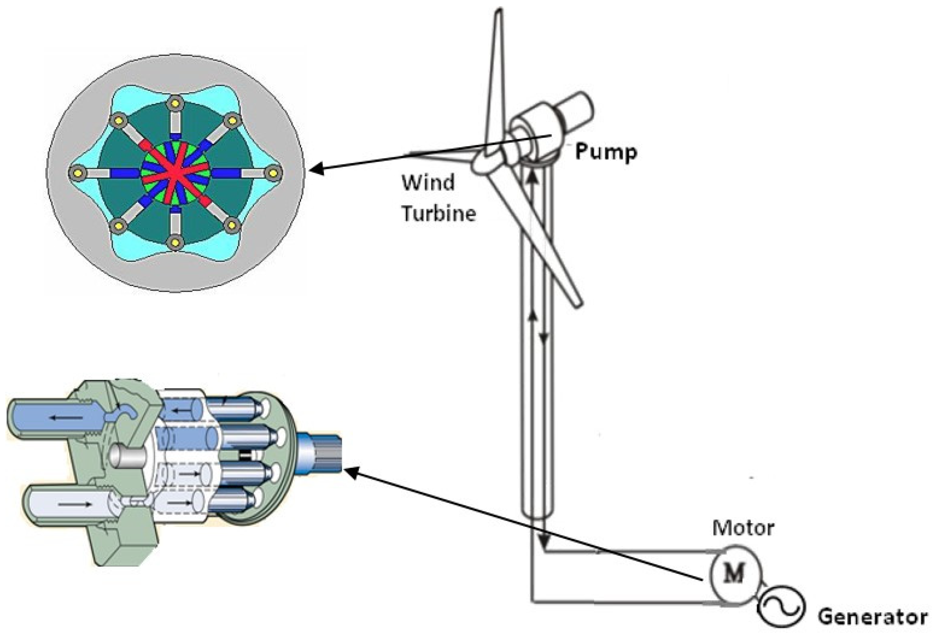
Figure 1 shows the schematic of a hydrostatic drive wind turbine (HSWT). Hydraulic pumps and motors are the key components in such a wind turbine. The rotor is the prime mover of the hydraulic pump. The pump provides a high-pressure flow through the pipes to the motor. The generator connected to motor applies a load torque through the motor shaft. This torque induces a pressure difference between the motor and the pump. The dynamics of the system are given by the following equation [
16].
2.1.1. Rotor
The wind power and turbine characteristics are as follows:
where
is the power generated from the wind,
is the power coefficient,
is the air density,
A is the swept area of the blades,
v is the wind speed,
is the optimal tip speed ratio,
is the pitch angle, and
is the angular velocity of the rotor. The torque applied on the pump is:
where
is the torque generated by the wind and applied to the rotor and pump,
,
is the displacement of the motor and pump,
is the pump pressure,
is the viscous drag coefficient,
is the Coulomb friction and
is the breakaway torque of the pump.
2.1.2. Fixed Displacement Pump
The angular velocity of the rotor is the same as the pump and since the pump has a fixed displacement, then the flow from the pump is:
where
is the dynamic viscosity of hydraulic fluid and
is the slippage coefficient of the pump. The fluid compressibility model gives the relationship between pressure changes and the amount of compressed flow in a control volume. This relationship is expressed as:
where
B is the bulk modulus and
,
is the flow of the pump and motor. The efficiency of the pump is given by:
where
,
, and
are the total, mechanical, and volumetric efficiency of the pump, and
A is a dimensionless factor.
Figure 2 shows the efficiency contours of compatible piston pumps used in wind turbine applications at different pump speeds and pressure variations. In our prior study, the designed MPPT controller regulated the pump speed in order for it to operate on the optimal efficiency line (dotted line in
Figure 2) [
16]. This is attained provided that pump rotor speed/torque characteristics match. This ensured that the pump efficiency was in the range of 93–94%, which is the maximum attainable efficiency for the pump for the given operating conditions.
2.1.3. Variable Displacement Motor
Similarly, for the variable displacement motor, the flow and the torque equations are:
The moment equation is:
where
is the load torque and the efficiency of the motor is:
where
B is a dimensionless factor. The motor efficiency can be written as:
where
,
, and
are motor efficiency constants (at fixed speed) and are:
Since the motor speed needs to be kept at a constant value in HTS wind turbine applications, its efficiency can be shown as a function of discharge pressure (
Figure 3). It is evident that the motor efficiency rises quickly to above 85% in pressure ranges over 100 bars. Therefore, the motor efficiency could always be kept at a higher value by maintaining a higher system operating pressure. In order to minimize the motor hydrostatic efficiency loss, this loss term needs to be included in the performance index to design the optimal controller.
2.2. Constrained Optimal Control via PMP
A performance index (PI) with quadratics terms is often used in deriving a control law through an appropriate optimization technique [
17,
18,
19]. A generalized performance index may include non-quadratic terms with constraints and penalties applied on the final states of the system. For a system such as
, a general PI can be expressed as [
16]:
The penalty imposed on the states at final time (
T) can be defined as: ∅(
x(T),
T)
. L(
x,
u,
t) represents the cost function that is to be minimized. The Hamiltonian value,
H, can be expressed in terms of the system model and the PI, as defined above as:
The optimal control law can be derived from the necessary optimality condition of the Hamiltonian value,
. The control law thus derived would generally be a function of both the states and the co-states. The following partial differential equations (PDEs) will need to be solved to obtain an explicit optimal control law:
It is assumed that the initial conditions,
are known and the boundary conditions associated with Equation (13) are given by:
Here, v represents the Lagrange multiplier of the final constraints. Equations (12)–(14) represent a generic time-varying system. f, L, and H will not be explicit functions of time if the system is a time-invariant system. The boundary conditions for the optimization of the final states and time are given by Equation (14). For cases where the time is not subject to optimization, it will be a constant, thus: dT = 0. Therefore, the second term in Equation (14) could be dropped since our objective was to minimize the overall loss in the HTS. Thus, the desirable PI will consist of rotor aerodynamic loss and HST loss.
Using the boundary conditions applied in [
16,
20], the cost function included the aerodynamic loss and hydrostatic loss
. A performance index can be written as:
The states are defined as
x1 = P;
x2 = ωp;
x3 = ωm and the controls are
u1 = Trotor,
u2 = Dm,
and u3 = Tload. Thus, the Hamiltonian values derived from (12) expressed with defined states and controls are given by:
The stationary condition,
, yields the control law as:
where,
is the optimal control and
λ*(1,3) denotes optimal co-states. Since
dT = 0, and the final constraints undefined, it can be set as
ψ(
xT) = 0; thus, the boundary conditions (14) can be further simplified as follows:
It is noted that the final penalty is on the system pressure,
x1. Therefore, the co-state
λ1 will be non-zero at final time:
It is to be noted that the PDEs in Equation (13), along with the boundary conditions in (19), need to be solved for the optimal state and co-state trajectories. The optimal trajectory for the control can be derived by substituting Equation (19) into Equation (17). Thus, a real-time optimal control law can be derived as follows:
The above control law would ensure a weighted minimization of the aerodynamic loss (first term), as well as the hydrostatic loss of the motor (second term). The weighting factor in the form of the ratio α1/α2 would dictate the contribution from each of the terms in (20).
2.3. Unconstrained Optimal Control
The output power from the HSWT can also be maximized though efficiency loss minimization via implementing an unconstrained optimization. This is a simplified approach compared to the Pontryagin minimum principle since a cost function is minimized by only considering the system dynamics model. Here, a weighted summation of the aerodynamic and transmission losses forms a cost function as follows:
where
is the penalty on aerodynamic loss, deviation from wind power MPPT, and
is the penalty on hydrostatic loss. Considering
, a pairing suggested by the RGA analysis,
Dm is desired as a function of
P [
21]. Hence, to find an optimal control law that minimizes the
J, a derivative using the chain rule can be applied:
In this derivative, the term
is the reciprocal value of the derivative of the motor displacement with respect to pressure. Since it is desired to derive a control law based on pressure feedback, then
is the reciprocal value of the control law derivative. Provided that it is non-zero, (22) can be deducted. Such an assumption needs verification after the control law is derived.
Hence, an optimal control law will be derived using
as follows:
From this derivative, a quadratic equation of motor displacement is obtained and an acceptable root of such an equation yields the optimal control law, as follows:
From this equation, it can be shown that is always non-zero so that the assumption of (22) is valid.
Equation (25) shows that the control law using pressure feedback depends on the ratio of As defined previously, is the weighing penalty on hydrostatic loss of the motor and is the weighing penalty on deviation from wind MPPT. To investigate performance of the control law proposed in (25), operation of a wind power plant using the HSWT introduced in previous sections was simulated.
3. Simulation Results and Discussion
As a test case, a 600 kW HTS wind turbine was selected for modeling and simulation purposes. This is a medium-size wind turbine with commercially available pump and motor sizes, for which the technical data were available at the time of this study. The specifications of this HTS wind turbine are provided in
Table 1 and
Table 2 [
22]. The relevant parameters have been used to simulate performance of the proposed optimal control law with the objective of maximizing the output power. Simulation runs were carried out with different ratios of
or
. A smaller ratio denotes dominancy of aerodynamic efficiency, while a larger ratio corresponds to dominancy of hydrostatic efficiency.
A series of wind speed steps were utilized to push the drivetrain system to its limit in order to verify the robustness of control system performance. Each speed level indicates the mean wind speed at the hub height and lasts for about 80 s. In total, a 60 min operation was simulated.
Figure 4 illustrates the wind speed step changes.
Both the model equations and the optimal control laws were implemented using MATLAB script. The same wind profile was used for simulating both the control laws.
It is to be noted that a zero value for or means that the control input is obtained by only minimizing the aerodynamic loss representing MPPT of the wind energy. The power outputs for this case establishes the baseline so that the other cases that include the minimization of drivetrain losses can be compared with the baseline. A non-zero value of this ratio would indicate the minimization of both aerodynamic and drivetrain efficiency losses according to this ratio.
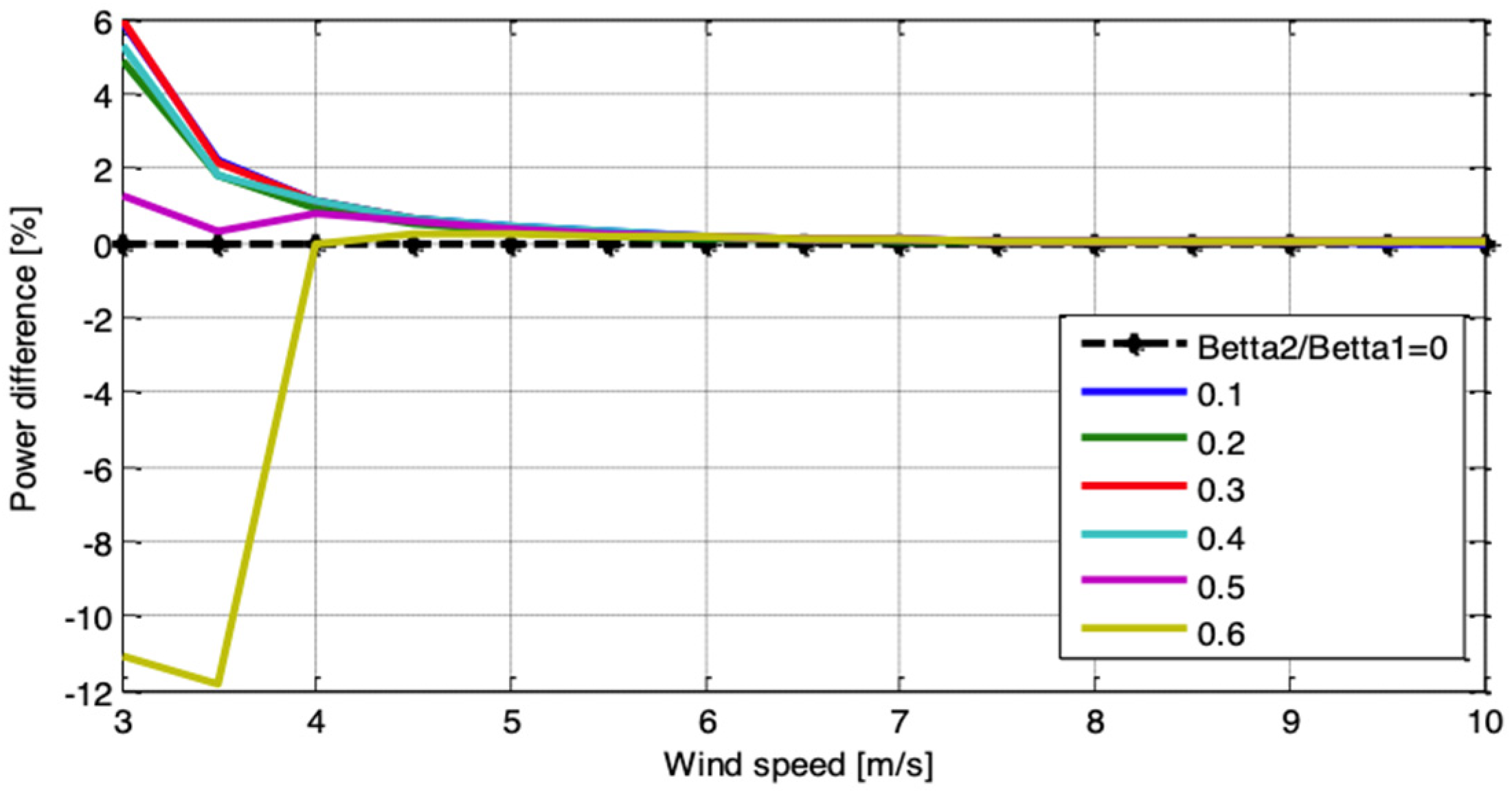
The constrained optimization control law (20) was first simulated with closed loop control on the HSWT plant model at various wind speeds for different
ratios. The results are captured in
Figure 5, which shows the output power difference (percent) between the PMP-controlled HTS and the baseline (with only MPPT control) at different wind speeds. It can be observed from this figure that for
values of up to 0.1, the output power shows a slight increase. However, for higher
ratios, the output power actually decreases.
Figure 5 also shows that the output power does not change with the weighing ratios for medium-to-high wind-speed ranges. The best ratio of maximum overall HSWT efficiency can be observed at 0.1.
Figure 6 shows the HTS efficiency differences between the PMP optimal control and the baseline MPPT control at various
ratios. It can be observed that at low wind speeds, the HTS efficiency is significantly higher compared to the MPPT baseline. At low wind speeds, higher
ratios improve the hydrostatic efficiency. This can be explained by referring to
Figure 2 and
Figure 3; at higher wind speeds, the turbine speed increases resulting in increased pump speed. According to
Figure 2 the pump discharge pressure would increase, resulting in higher system pressure. As a result, the motor pressure increases giving rise to motor efficiency. The gradient of motor efficiency is higher at low wind speeds, so even slightly higher pressure improves the efficiency noticeably. For moderate-to-high wind speeds, the efficiency of the motor reaches its maximum value. Another observation is that for the whole range of wind speeds, there is a trade-off between maximum power harvesting at the rotor (MPPT) and maximum efficiency of the hydrostatic transmission. So by choosing the
ratio appropriately at low and moderate-to-high wind-speed ranges, it would be possible to have the entire HSWT plant operate optimally.
Next, the unconstrained optimal control law (25) was simulated in a closed loop with the HSWT plant model at various wind speeds and
ratios. Again, a zero
ratio indicates MPPT baseline simulation. The difference in power generation for different weighing ratios and the baseline is shown in
Figure 7, where the trend of output power variation is similar to that observed in the PMP control law results shown in
Figure 5. It can also be observed here that a slightly improved output power can be achieved by increasing the weighing ratio up to 0.3 in this case. For higher weighing ratios, the trend of power difference becomes reversed.
To further compare improvements between the PMP control law (20) and the unconstrained controller (25), the best weighing ratio for each controller was chosen (in a low speed region). For the PMP control law, the best ratio was 0.1, while for the unconstrained optimal control, the ratio was 0.3. The differences in power output for each controller at their respective best weighing ratios with respect to the MPPT baseline are shown in
Figure 8. It can be observed that the output power difference for the optimal controller that minimizes the overall loss (PMP or unconstrained) and the baseline MPPT is positive in low wind-speed regions. At very low wind speeds (3–4 m/s) both constrained and unconstrained controllers perform about the same. At higher speeds (4–6 m/s) constrained controller has a little advantage over unconstrained one. In the wind-speed region of 6–9 m/s, the unconstrained controller offers better results with respect to power output.
For the selected 600 kW HSWT system, additional simulation results were generated to obtain additional energy that could be generated using the proposed control strategies over the MPPT baseline for the given wind profile for a period of one hour (
Figure 4).
Figure 9 shows the comparison of energy harvested in a one-hour period for all three cases: MPPT baseline, PMP controller, and unconstrained controller. The energy produced using the unconstrained optimal control law can be seen to be higher than that produced using the constrained optimization and the MPPT.
The above simulation results show that there is a potential for the proposed optimal controllers to improve the output power for a HTS wind turbine in low speed ranges.


