Thermal Switch Based on an Adsorption Material in a Heat Pipe

Abstract

For many applications, the possibility of controlling heat flow by “thermal switching” could be very beneficial. Several concepts for heat switches were already proposed and tested, however, many drawbacks of these concepts are evident. In this work, we present a novel approach for thermal switching using a water-loaded adsorbent as part of the evaporator of a heat pipe. The basic idea is that the adsorbent releases water upon exceeding a certain evaporator temperature, and thus “activates” the heat pipe by providing the working fluid for thermal transport. The first part of this work concentrates on the adsorbent characterization by analyzing the adsorption isobars and isotherms and thus understanding the behavior of the system. Furthermore, a model to predict the release of water from the adsorbent in dependence of temperature was developed. Subsequently, the adsorbent was integrated into an actual heat pipe demonstrator to verify these predictions and demonstrate the thermal switching ability. Overall results revealed a very good agreement between the predictions concerning water release and the heat pipe’s thermal behavior. The obtained thermal switching ratio depends on the heating power and temperature range that is considered. Depending on whether evaporator/condenser or the adiabatic zone are considered, average switching ratios of circa 3 and 18 were found, respectively.

1. Introduction

For many applications, the possibility of controlling heat flow by “thermal switching” could be very beneficial. It would enable the user to set a desired thermal resistance for a heat-conducting object or switch between a heat-conducting “on-state” and a heat-blocking “off-state”. Such a heat switch would have great potential in thermal management in a wide variety of applications to improve efficiency and reduce costs, for example in systems related to energy storage and transport. In addition, effective thermal switching is a necessary prerequisite to enable efficient caloric heat pumps with sufficient cooling power [1]. As detailed for example in a recent review article by Wehmeyer et al. [2], numerous concepts exist for such thermal switches, based on many physical mechanisms and approaches: conduction-based switches (such as solid–solid contacts, liquid bridge switches, thermal expansion, materials with changing thermal conductivities in different phases, etc.), convection-based switches (based on fluids, heat pipes, jumping droplets, electrowetting, etc.) and radiation-based switches.

The basic characteristic of a thermal switch is the achieved on/off ratio or switching ratio $r=G_{on}/G_{off}$ (where $G_{on}$ and $G_{off}$ are the thermal conductance in the on- and off-state, respectively). The achieved switching ratios can vary over a wide range from 1.1 to over 500. If the device works in a sense of a thermal diode rather than a thermal switch, the rectification $\gamma =\frac{G_{fwd}-G_{rev}}{G_{rev}}$ (where $G_{fwd}$ and $G_{rev}$ are the thermal conductances in forward and reverse direction, respectively) is the characteristic property.

A special subgroup of heat switches are thermal switches and diodes based on heat pipes (HPs). The simplest concept is a thermosyphon, in which gravity provides the asymmetry [3]. One method to realize a thermal diode that is strongly anisotropic thermal transport without the aid of gravity is to design a heat pipe with asymmetric shape. Different thermal diode concepts were proposed in the literature [2,3]. One example is the liquid trap diode proposed by Groll et al. [4]. This diode has an asymmetric shape with a liquid trap appended on one end of a traditional heat pipe. With this design, large rectifications of circa 300 in combination with a high forward-mode conductance of 13.8 W/K are possible. Another approach is to create a jumping droplet thermal diode. In the forward mode, the vapor evaporated from the hot superhydrophilic surface condenses on the cold superhydrophobic surface and the liquid is efficiently returned to the hot side by droplet jumping or surface tension forces. In the reverse mode, this mechanism of liquid return is blocked. The concept was realized by different research groups yielding rectifications between 2 and 150 depending on experimental conditions [2,5,6].

For thermal switches, different concepts are used. One widely studied concept is the variable conductance heat pipe (VCHP). Here, a volume of non-condensable gas (NCG) blocks the condenser at low evaporation temperatures effectively suppressing recondensation of the fluid. At higher temperatures, the NCG volume is compressed such that the effective area for condensation is increased with positive effects on the heat pipe’s thermal conductance. Altogether, upon exceeding a certain evaporator temperature threshold, the conductance increases very abruptly, effectively leading to switch ratios of circa 200 [2,6]. Finally, one can combine a heat pipe with a solid–solid contact to design a thermal switch. This can be done for example by attaching the heat pipe to a spring system, consisting of standard “bias springs” and additional springs made of shape memory alloy (SMA) that counteract the bias springs [7]. Due to phase change in the SMA above a certain threshold temperature, the force of the SMA springs is overcome by the bias springs and the heat pipe connected to the SMA springs is extended together with the springs forming a solid–solid contact with the object to be cooled (in this case, a liquid oxygen tank on the lunar surface).

To conclude, numerous different concepts can be used to realize a heat switch. However, many of these concepts exhibit drawbacks. For example, the solid–solid contact-based switches tend to be bulky and complex, consist of several moving parts, have a thermal resistance that is too high in the conducting state of the switch or an active element such as an electrical power source is necessary to switch between the conducting and non-conducting state. The heat pipe diode-based concepts were shown to achieve high rectifications; however, it is difficult to exchange the forward and reverse directions of the heat flow, which is necessary to effectively enable a heat switch action. True heat switches were achieved with VCHPs, however, the VCHP performs worse than a standard HP due to the effect of the NCGs. This is particularly evident as soon as the HPs exhibit an adverse-gravity orientation, even for small inclination angles [8].

In this work, we present a novel approach for thermal switching using a water-loaded adsorbent integrated in a heat pipe, or more exactly, a thermosyphon (Figure 1). The adsorbent releases significant amounts of water by desorption as soon as a certain temperature threshold is exceeded, and the released water can subsequently serve as the working fluid in the heat pipe for latent heat transport. This in turn enables a significant reduction in the heat pipe’s thermal resistance as soon as a certain temperature threshold or switching temperature $T_S$ is exceeded. This approach to enable a heat switch is passive (for example it does not require external forces such as mechanical force or electricity), has no movable parts, does not require NCGs, can be miniaturized and is very cost-efficient.

To realize the heat pipe-based switch, we first consider the water loading behavior of a special adsorbent with respect to heat pipe working conditions by analyzing the adsorption isotherms and isobars. Using these data, it is possible to estimate the switching temperature $T_S$ as defined above. Finally, a demonstrator of the switchable heat pipe was set up and tested, confirming the predicted thermal behavior and the estimation of $T_S$ based on the measured adsorption isotherms.

2. Experimental Setup

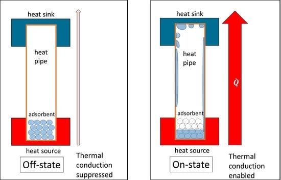
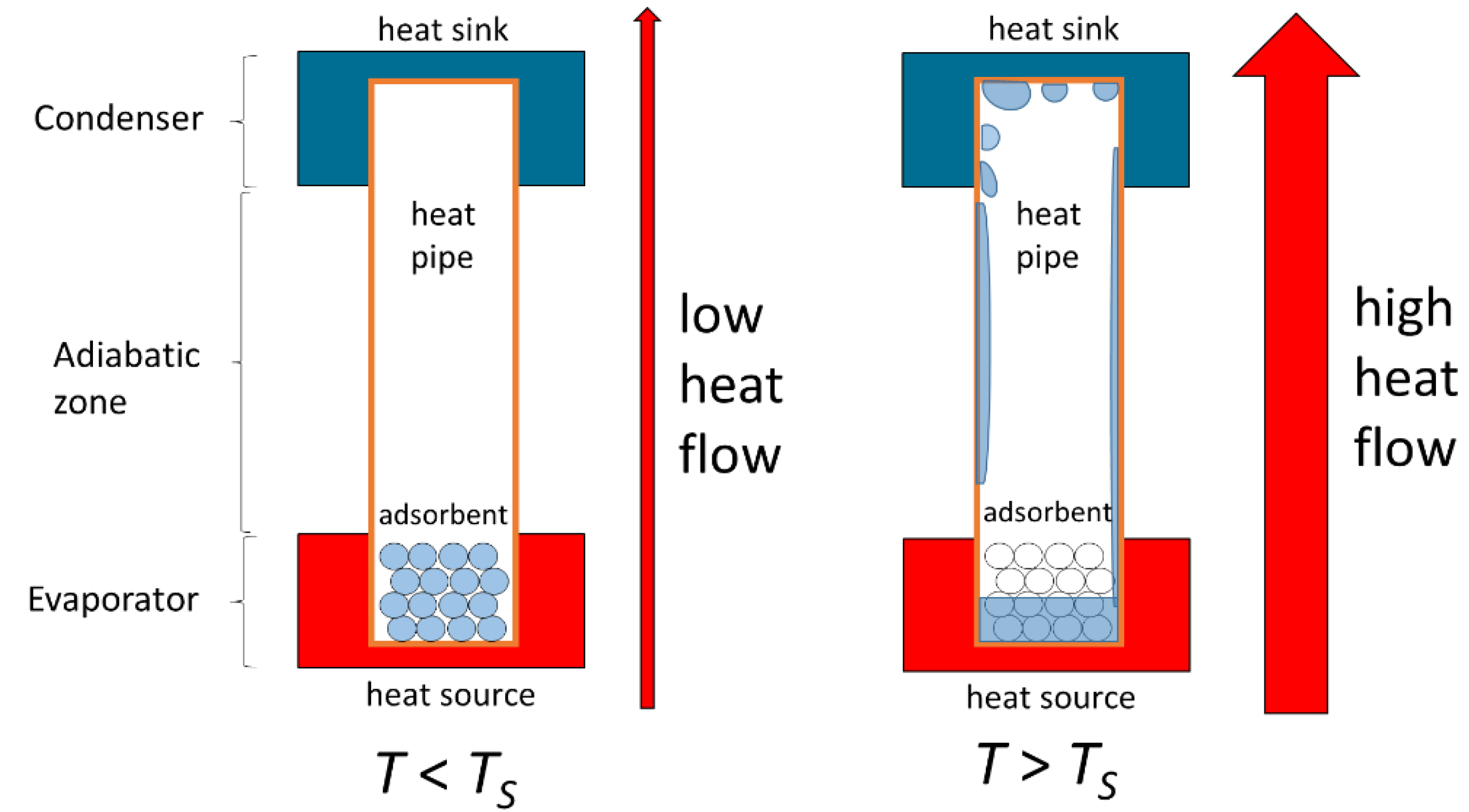
2.1. Basic Concept

The amount of water or adsorptive bound per adsorbent is referred to as the loading x of the adsorbent. The loading depends on the adsorbent’s temperature T and the pressure p of the working medium in the gas phase and x = f(T, p). Adsorption equilibria are usually represented by adsorption isotherms. An adsorption isotherm is a curve that relates the loading of an adsorbent to the pressure of the adsorptive at a given temperature (x = f(p), T = const).

For the intended application, the adsorbent must release the bound water as abruptly as possible when a specified temperature is reached. This condition is satisfied if the material exhibits so-called type IV and V isotherms that exhibit a sharp change in adsorbed amount of water as shown in Figure 2.

The adsorption material fulfilling these requirements and therefore used in this work is a titano-silico-alumino-phosphate (TAPSO-34) from Clariant Produkte GmbH (Germany). TAPSO-34 is a zeotype adsorbent with chabazite structure which is formed by corner-connected AlO₄, PO₄, TiO₄ and SiO₄ tetrahedral units [10]. The material has similar adsorption properties as the well-known SAPO-34 [11] and AQSOA FAM-Z02 [12,13]. One of the main differences between the materials is the better hydrothermal stability of TAPSO-34 when compared to conventional SAPO-34. This is an important property for the present application, as the material is expected to be exposed to liquid water at elevated temperatures.

The water adsorption properties of pure TAPSO-34 were already investigated by Kohler et al. [14] and published as isotherms (Figure 3). The isotherms agree with the type V classification as can be seen from the convex slope at low pressures of the 85 °C isotherm. Altogether, because of this adsorption behavior, TAPSO-34 was selected to be a well-fitting material for the construction of a thermal switch when inserted into a heat pipe.

The basic concept of the heat pipe-based thermal switch is that the activation is governed (i) by the temperature of the evaporator which contains the loaded adsorbent and (ii) the temperature and resulting vapor pressure in the condenser, where the condensation of the working fluid takes place. This is illustrated in Figure 3. If the temperature at the condenser of the heat pipe is for example fixed to 30 °C using air or water cooling, the vapor pressure of the working fluid in the condenser zone should correspond to the vapor pressure of the working fluid at 30 °C (dashed line in Figure 3). If, for example, the temperature of the loaded adsorbent in the evaporator zone is raised from 35 to 60 °C, only a small amount of water is desorbed ($∆x_1$) which is most likely not sufficient to activate the heat pipe. If the temperature of the evaporator zone is further raised to 85 °C, significantly more water is desorbed ($∆x_2$), which should lead to an activation of the heat pipe.

2.2. Preparation and Characterization of Adsorbent

To insert material into the system, we used granular TAPSO-34 with a binder content of 20% and a grain size in the range of 1.5 to 3 mm instead of pure TAPSO-34 powder. The granulation was carried out by the manufacturer directly. This material may have different adsorption properties than pure TAPSO-34 powder and is therefore characterized again in detail in this work.

2.2.1. Pre-Treatment of the Adsorbent

For the correct operation of the heat pipe, a certain quantity of free working medium is needed. To ensure that this quantity of free working medium is available under certain operating conditions, the amount of working fluid (water) in the adsorbent must be precisely adjusted. For this reason, the adsorbent was subjected to a pre-treatment procedure before it was inserted into the heat pipe. The adsorbent was first evacuated in a vacuum oven (Memmert, VO400) at 200 °C and absolute pressure of 1 kPa for 3 h to desorb any undesirable substances. Afterwards, approximately 50 mL of the material was stored at 20 °C and a relative humidity of 43% for 3 weeks to set a defined water loading. The pre-treatment conditions were chosen to be not sensitive to small changes in either temperature or relative humidity. The relative humidity was adjusted by a saturated solution of potassium carbonate [15]. A sample container with a volume of approximately 50 mL was filled with granular TAPSO-34 and placed in a bigger sample vessel, which contained the salt solution at the bottom (see Figure 4). The whole set-up was placed in an air-conditioned laboratory at a temperature of 20 °C. Altogether, the procedure resulted in a water loading of 21.6%.

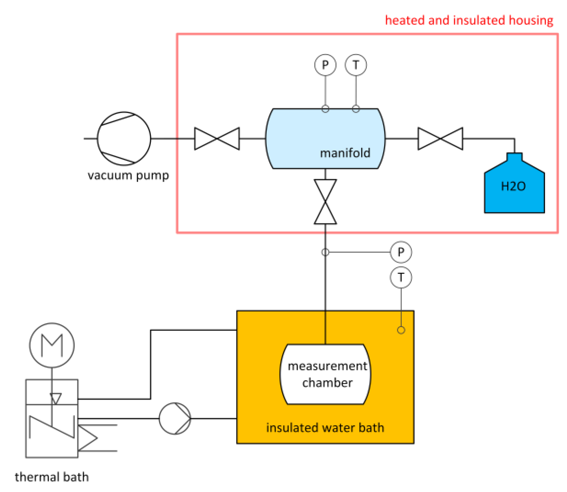
2.2.2. Measurement of Adsorption Isotherms

Water adsorption isotherms were measured at various temperatures ranging 20–85 °C using a Quantachrome Autosorb iQ surface area analyzer (Figure 5). In this setup, the porous sample is placed in the measurement chamber, the temperature of which is controlled via an insulated water bath with an accuracy of ±0.5 K. Liquid water is evaporated in a steam generator and dosed via a gas manifold into to the measurement chamber. From the pressure drop in the manifold, the adsorbed amount of water vapor is determined. The gas manifold is heated to 50 °C to avoid condensation. Samples—if not stated otherwise—were degassed in vacuum for 12 h at 200 °C prior to the analysis.

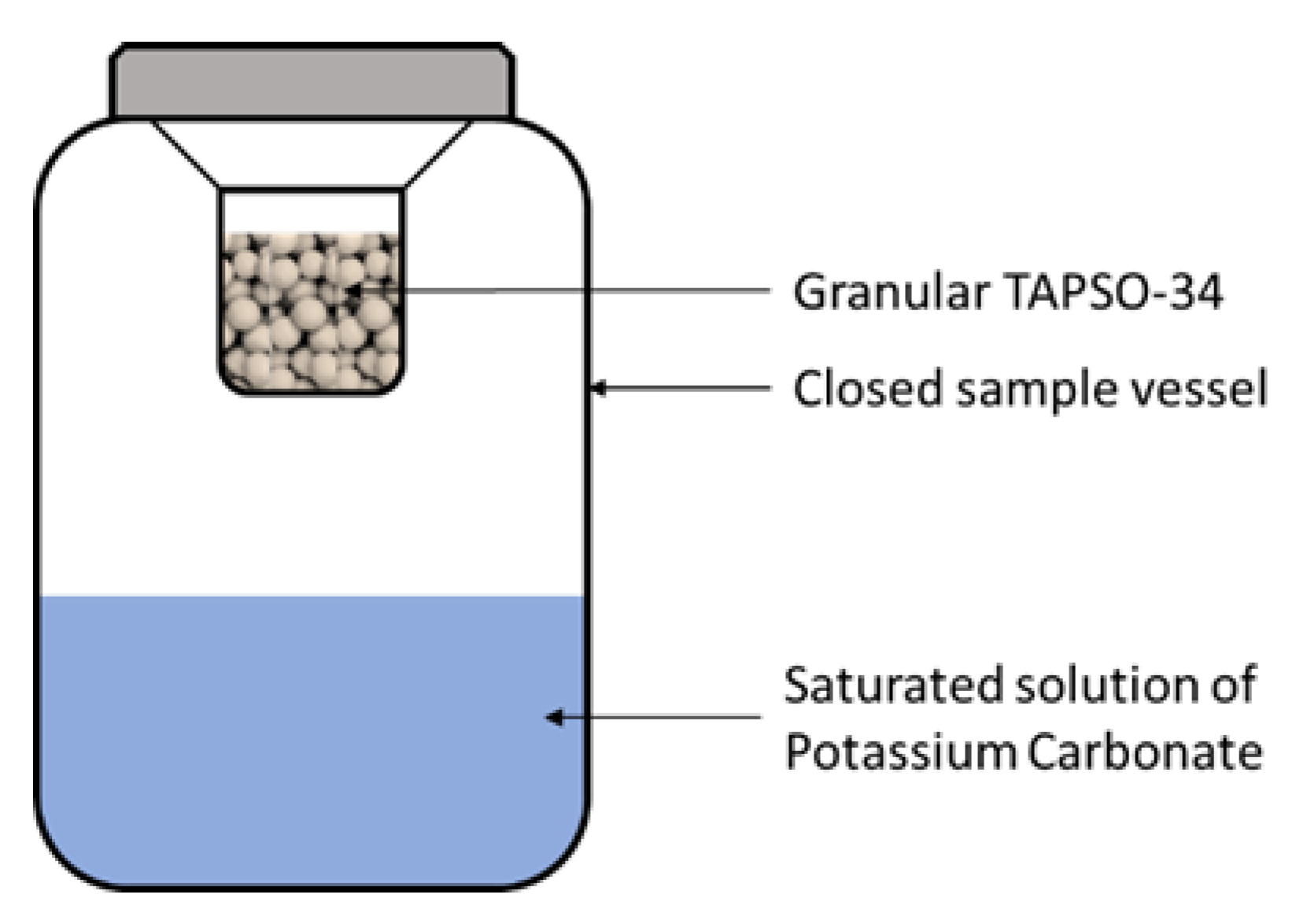
2.2.3. Measurement of Initial Water Loading and Adsorption Isobars

A small sample of the adsorbent with a mass of approximately 300 mg was placed in a magnetic suspension balance (Rubotherm, IsoSORP) to measure the water content after the pre-treatment procedure and adsorption isobars for the validation of the adsorption model, which is presented below.

The magnetic suspension balance used has a closed measuring cell in which the sample is placed in a sample container (Figure 6). The weighing unit is located outside of the measuring cell, and the force transmission takes place via an electromagnet. This design has the advantage that the sample can be examined in a wide pressure and temperature range, while the sensitive load cell is only exposed to laboratory conditions. The resolution of the load cell is 10 µg, the accuracy is specified as 20 µg. A reference weight is integrated and automatically used to determine the density of gas used and perform a buoyancy correction. A gas dosing system is connected to the measuring cell, via which pure gases (helium, argon, nitrogen, synthetic air, etc.) and mixtures of these gases can be supplied continuously. The system is also capable of providing humid air to study vapor adsorption. For this purpose, liquid water is dosed via an HPLC pump into an evaporator, which is placed in the inlet gas stream.

The initial loading of the adsorbent after the pre-treatment was determined by drying the sample for 3 h at 250 °C in a dry nitrogen atmosphere.

Adsorption isobars were measured at vapor partial pressures of 3.17 kPa and 4.01 kPa. For this purpose, the sample was initially dried for 3 h at 250 °C in a dry nitrogen atmosphere and then saturated at 35 °C and the corresponding partial pressure of water vapor. The water vapor pressures were adjusted by dosing 5 µL/min of liquid water into a dry nitrogen gas stream of 386 and 305 sccm, respectively. The temperature was then raised stepwise from 35 °C to 45 °C, 55 °C, 65 °C, 75 °C, 90 °C and finally to 110 °C. Each measurement sequence, (segment) was terminated when no further change in the weight of the sample was observed.

2.3. Setup for Heat Pipe Demonstrator

2.3.1. Setup

A schematic of the heat pipe demonstrator is shown in Figure 7. The demonstrator consisted of a wickless borosilicate glass heat pipe (a thermosyphon) with a wall thickness of 1.8 mm, filled with the adsorbent TAPSO-34. As the heat source, a wire heater was used. The heater was immersed in a thermal oil bath (silicone oil Thermo Fisher A12728) contained in a glass beaker (insulated with wrapped polyethylene foam sheets) to homogenize heat input along the evaporator zone. We use the approximation that the heating power $\dot{Q}$ corresponds to the electrical power applied to the heater. At the condenser zone, a circulating water cooler was used to remove the heat from the heat pipe. The adiabatic zone was thermally insulated with a pipe insulation sleeve made of polyethylene foam. Type K thermocouples (OMEGA Engineering, wire diameter of 80 µm and Teflon insulation) were attached at defined positions along the adiabatic zone and at the wire heater and cooler as described in the caption of Figure 7. For measurement error analysis, it is crucial to consider the uncertainties in the used temperature measurement devices since this defines the uncertainty of the obtained experimental values. The uncertainty for absolute temperature measurement using a single Type K thermocouple in accuracy class 1 is specified as ±1.5 °C. This is also the absolute temperature uncertainty that applies to the data shown in Section 3.2.1 and Section 3.2.3. However, for calculating the thermal resistance as shown in Section 3.2.3, not absolute temperatures but actually temperature differences were used. To minimize the measurement error for temperature differences, the thermocouples used in the experiment were selectively taken from the same production batch such that when all subjected to the same temperature simultaneously, the scatter of the measured temperatures corresponded to a standard deviation of only circa ±0.3 °C. This scattering was then interpreted as the uncertainty for the measurement of temperature differences $\mathsf{\Delta }{T}_{HC}$ and $\mathsf{\Delta }{T}_{ad}$ (as defined in Equations (9) and (10) below). The uncertainty of the temperature difference measurement then yielded the uncertainty on the obtained thermal resistances $R_{th-HC}$ and $R_{th-ad}$ (as defined in Section 3.2.3). In the adiabatic zone and particularly at low powers, the observed temperature differences were very small when the heat pipe was in the “on”-state and thus, a large relative measurement uncertainty resulted, as can also be seen in Section 3.2.3 (large error bars on thermal resistance in adiabatic zone).

The length of the evaporator (given by the thermal oil bath), adiabatic and condenser zone was 7, 13 and 12 cm, respectively. Of the pre-treated TAPSO-34, 7.15 g were loaded into the heat pipe, corresponding to a water loading of 1.27 mL (considering a loading of 21.6% as mentioned above).

2.3.2. Experimental Procedure

The pre-treated TAPSO-34 was taken out of its air-tight container and immediately filled into the glass heat pipe container. Then, the heat pipe container was evacuated for 15 min via a turbo pump connected by the ball valve shown in Figure 7. During the evacuation sequence, the adsorbent was kept at a temperature below 0 °C to avoid water desorption and subsequent removal from the system by the vacuum pump system. After the evacuation sequence was complete, the ball valve was closed again. During the experiments with the heat pipe, the valve was heated in order to avoid water deposition in the valve.

When the evacuation was finished, the ball valve was closed, and the heat pipe was allowed to settle until the adsorbent was at room temperature again. Subsequently, in eight consecutive steps and in ascending order, heating powers $\dot{Q}$ of 2, 3, 4.2, 6.9, 8, 10.7, 24.3 and 30 W were applied to the heaters, respectively, until the temperature stabilized for each power level. Simultaneously, all temperatures measured by the thermocouples shown in Figure 7 were recorded.

3. Results and Discussion

In this section, the results and discussion are presented separately for the adsorbent material (Section 3.1) and for the resulting heat switch demonstrator that is based on this adsorbent material (Section 3.2).

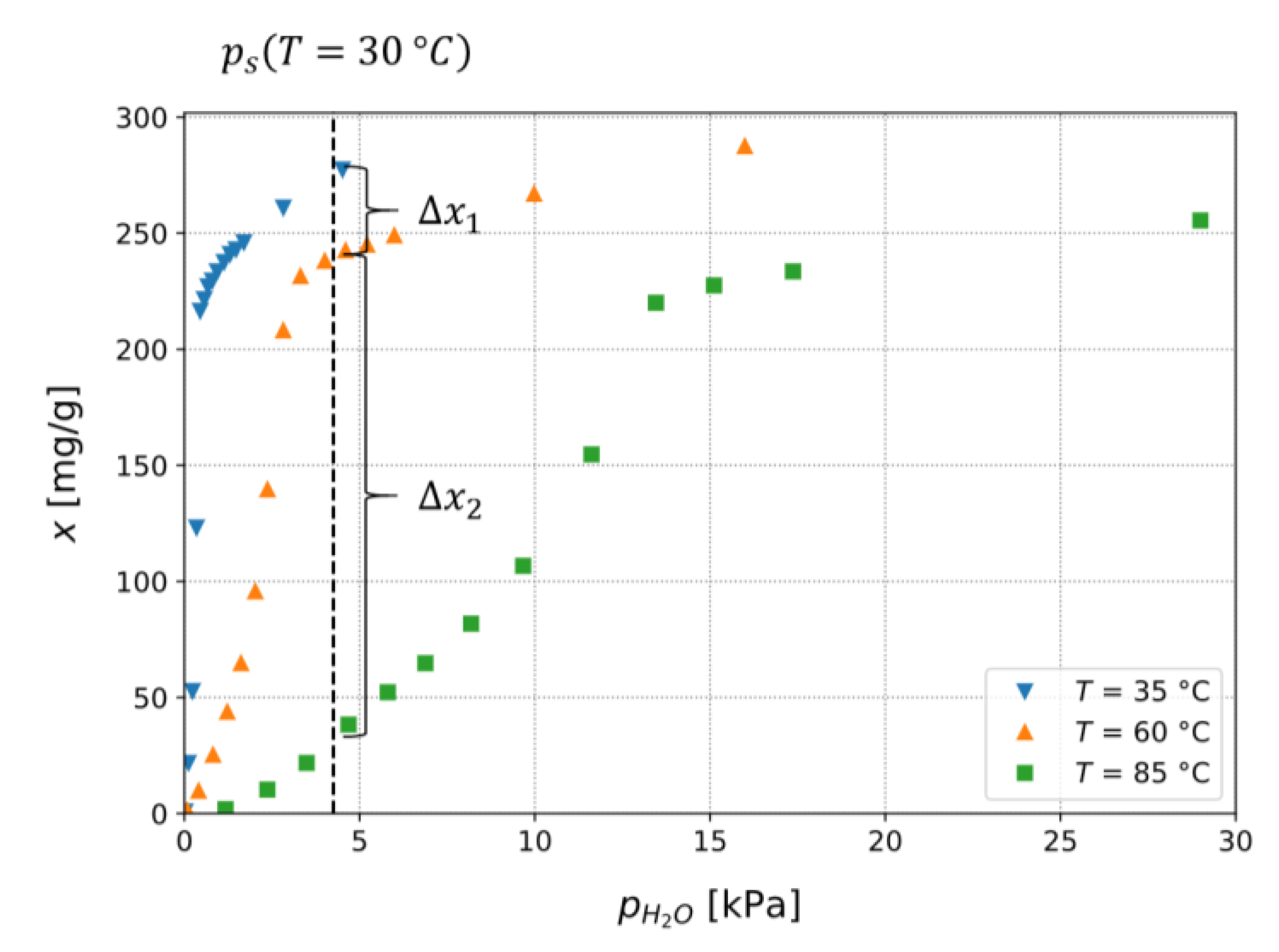
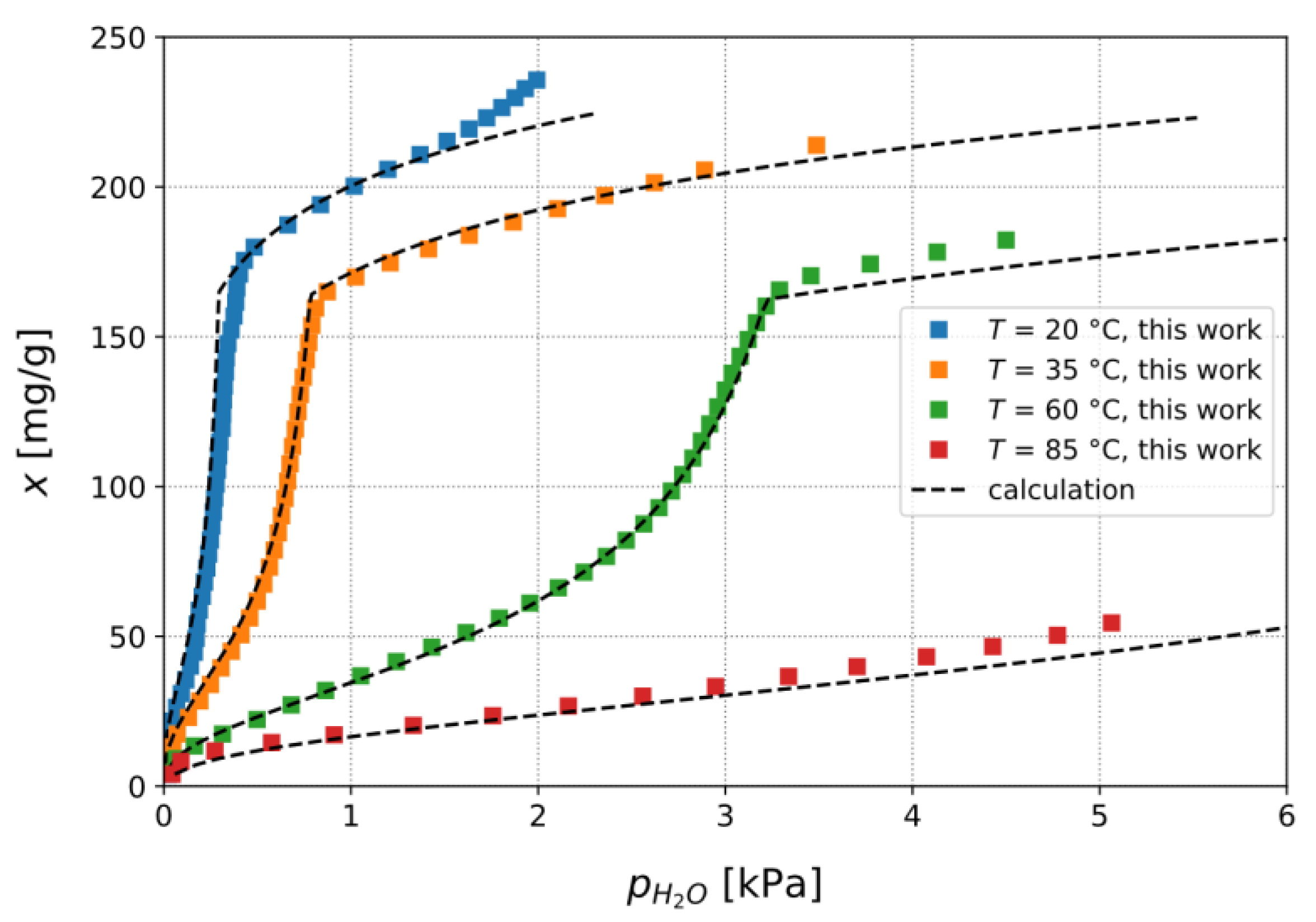
3.1. Adsorption Isotherms of TAPSO-34 and Estimation of Switching Temperature T_S

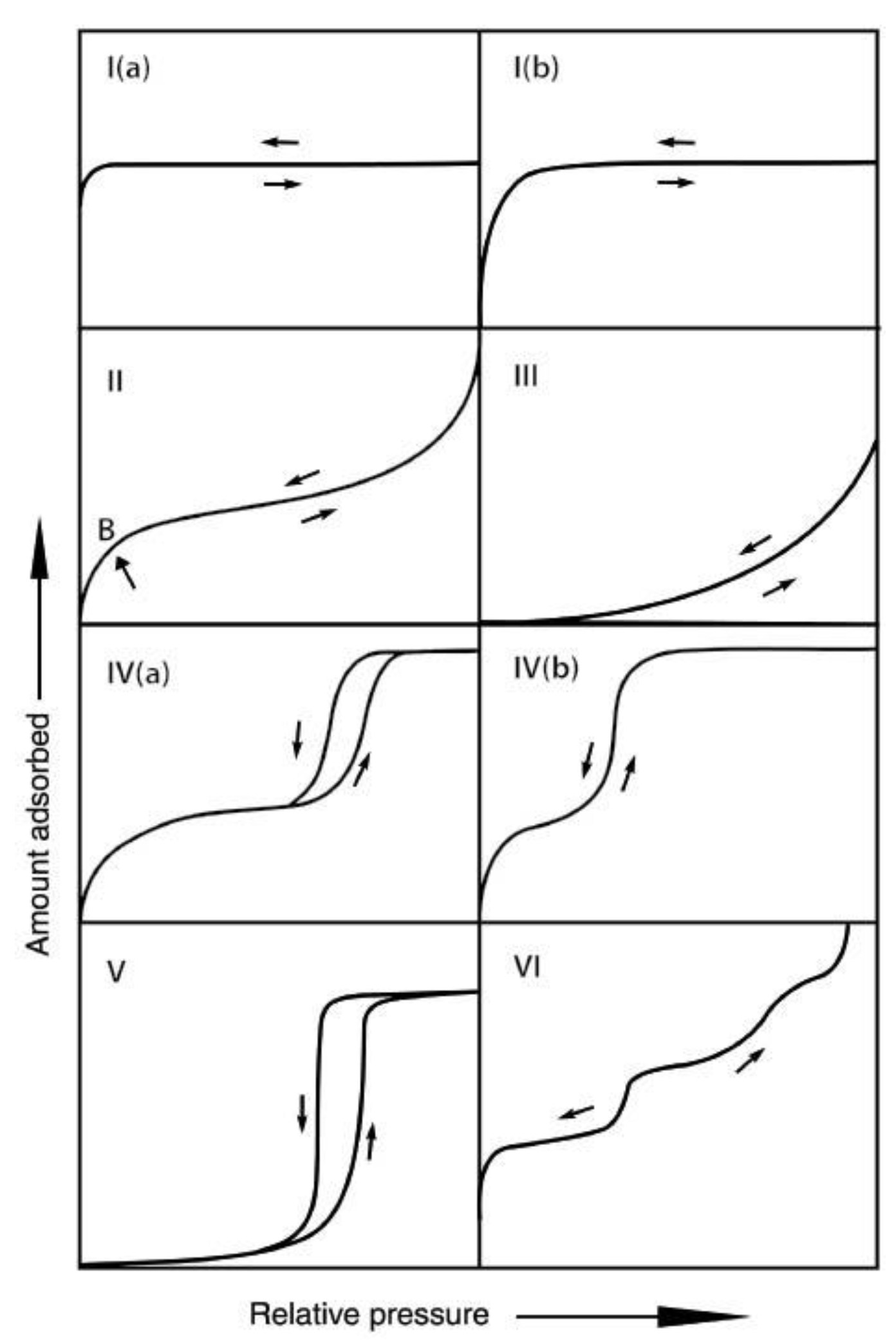
3.1.1. Adsorption Isotherms and Their Role in a Heat Pipe-Based Thermal Switch

Using the setup mentioned above, adsorption isotherms of water in TAPSO-34 were determined (see Figure 8). We note that the isotherms measured in this work differ from those given in the literature by Kohler [14]. The main reason for the deviations is the binder content of approximately 20% in the material used in this work, which leads to a lower adsorption capacity when compared to the pure adsorbent. Adsorption may also take place in the porous binder, which can lead to small differences in the shape of the isotherms. Small deviations may also occur from uncertainties in the sample temperature of different measurement systems.

The adsorption isotherms themselves, however, are not suitable for calculating the activation temperature of a switchable heat pipe. Rather, isobars describing the loading of the adsorbent at constant partial pressure, which relates to the vapor pressure of the adsorbent at the heat pipe heat sink temperature, would be useful. From such an isobar, the activation temperature of the heat pipe (where large amounts of working fluid are suddenly available for heat transport) could directly be estimated. Therefore, a method was developed that allows the calculation of isobars from the measured isotherms and is described in detail in the following subsection.

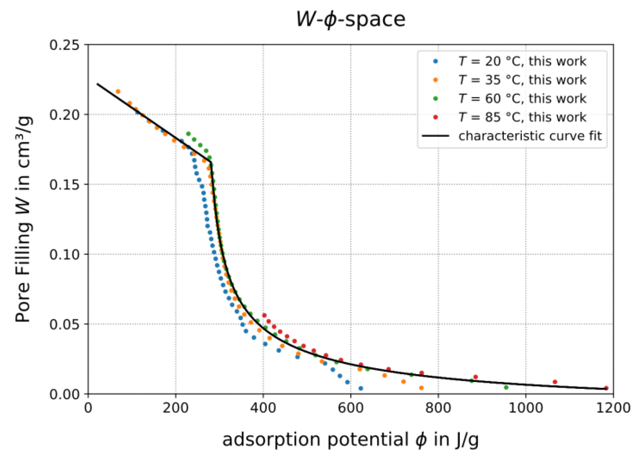
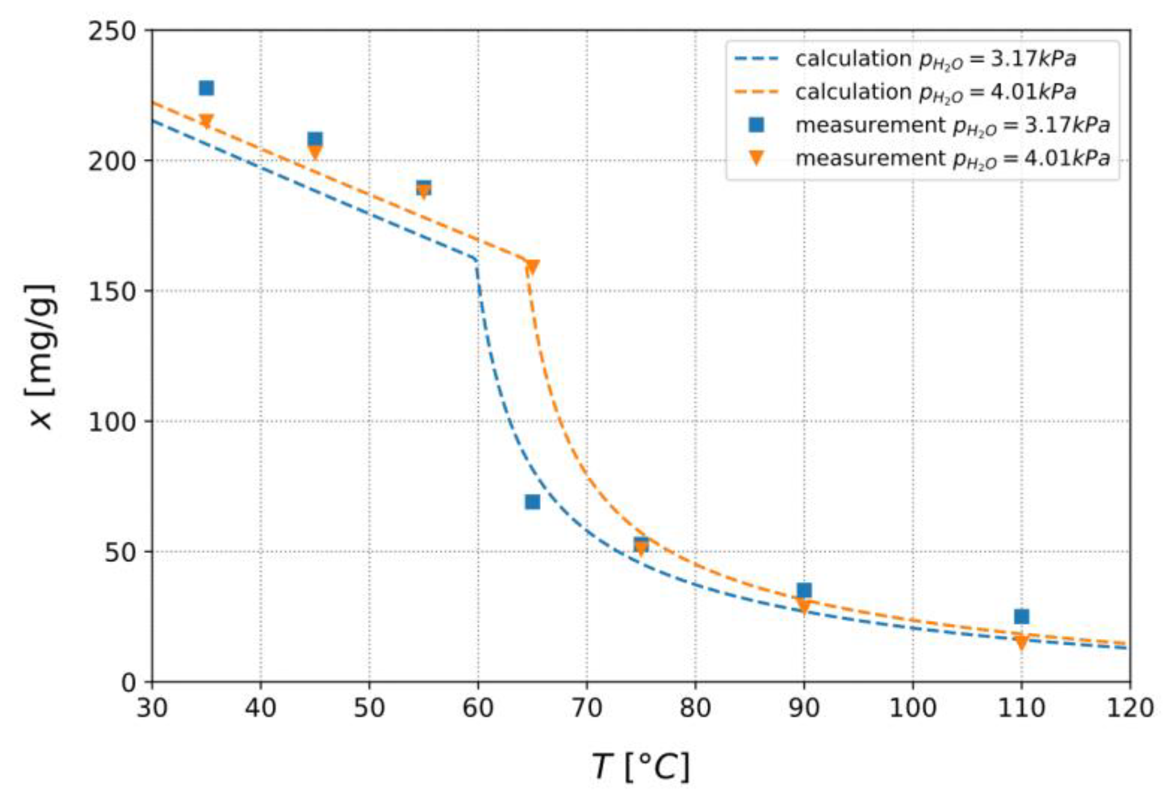
3.1.2. Calculation of Isobars from Measured Isotherms

The potential theory of Polanyi [16,17] modified by Dubinin [18] is suitable to calculate the loading of the adsorbent at almost every point in the p, T-space from only a few isotherms. Although this approach has limited accuracy and physical correctness at very low and very high partial pressures when compared to the vapor pressure of the pure adsorptive, it is very useful in many engineering applications [19].

Conventional adsorption models, for example the Langmuir adsorption model [20], are often derived using the covered surface area of the adsorbent. The basic idea of the potential theory is that adsorption in microporous adsorbents with pores in the dimension of the adsorbed molecules can be described by the filled pore volume rather than the covered surface area. The filled pore volume W of the adsorbent is given by:

$$W=\frac{x}{{\rho }_{Ads}\left(T\right)}$$

(1)

Here, ${\rho }_{Ads}$ is the density of the adsorbed phase, which is not directly accessible to measurements. In the present case, water is the adsorbent for which an approach for the adsorbate density is given by Hauer [21] that is used in many studies, for example [22]. Since we do not need to extrapolate the adsorbate density to temperatures above the normal boiling point of liquid water, we use the established model of Hauer and refrain from comparing different adsorbate density models. According to Hauer [21], the adsorbate density is then given as:

$${\rho }_{Ads}={\rho }_W\left(T_0\right)·\left(1-3.781·{10}^{-4}\frac{1}{K}·\left(T-T_0\right)\right)$$

(2)

with $T_0=283.15 \mathrm{K}$ and ${\rho }_W\left(T_0\right)=998\frac{\mathrm{kg}}{{\mathrm{m}}^3}$.

One of the main ideas of the potential theory is that there is a temperature-independent adsorption potential $\varphi$. This adsorption potential was defined by Polanyi as follows:

$$\varphi =RT\ln \left(\frac{p_s\left(T\right)}{p_a\left(W,T\right)}\right)$$

(3)

Wherein $p_s\left(T\right)$ is the vapor pressure of the pure adsorptive at the given temperature and $p_a\left(W,T\right)$ is the vapor pressure of the adsorbate at filled pore volume W at the same temperature. At adsorption equilibrium, $p_a$ corresponds to the partial pressure $p_i$ of the adsorptive in the gaseous phase, which in the present case is the partial pressure of water, $p_{H_{2}O}$. Hauer [21] shows that this adsorption potential is equivalent to the free enthalpy (or Gibbs free energy), as well as the Helmholtz free energy for ideal gases. Using Equations (1)–(3), the filled pore volume and adsorption potential can be calculated for each point of a sorption measurement. The results can be displayed in the so-called W-ϕ-space (see Figure 9a).

In many cases, points calculated from isotherms of different temperatures coincide to form a single curve in W-ϕ-space, also called the characteristic curve. Kohler [14] reported that this would not be the case with TAPSO-34 and thus proposed an extension to the potential theory. The idea is to replace the vapor pressure of the pure adsorptive $p_s$ in Equation (3) by a pressure he called desorption pressure $p_{des}\left(T\right)$. The starting point of this consideration is that the adsorbate has a different enthalpy of vaporization than the pure adsorbent. According to the Clausius-Clapeyron equation, the vapor pressure curve of the adsorbate therefore has a different slope. The difference of the enthalpy of vaporization of pure adsorptive (in the present case water) $∆h_{vap,water}$ and adsorbate $∆h_{ads}$ corresponds to the binding energy $∆h_b$ of the adsorptive and can be assumed to be independent of temperature in a first approximation. For the adsorption of water by TAPSO-34, Kohler assumes that the binding energy $∆h_b$ is approximately equal to the enthalpy of fusion of ice $∆h_{m,ice}$. If 0 °C is chosen as the reference temperature) $T_0,p_{des}\left(T\right)$ is obtained from the integrated Clausius-Clapeyron equation:

$$p_{des}\left(T\right)=p_s\left(T_0\right)·\exp \left(\frac{∆h_{ads}}{R_s}\left[\frac{1}{T_0}-\frac{1}{T}\right]\right)$$

(4)

$$∆h_{ads}\approx ∆h_{vap,water}\left(T_0\right)+∆h_{m,ice}\left(T_0\right)$$

(5)

The results of the potential theory by Polanyi and the modified potential theory by Kohler are compared in Figure 9a,b. For the further calculation of adsorption equilibria, it is important that, if possible, all measured adsorption points coincide to form a single curve. In this context, Polanyi’s adsorption potential is more suitable for the present adsorption material than Kohler’s since the measuring points of the different adsorption isotherms can be described more unambiguously by a single curve. Thus, we use the potential by Polanyi for further calculations in this work.

The characteristic curve must be described by an analytical function if it is to be used as a starting point for further calculations. For this purpose, different functions were used in the literature, among them the Dubinin-Astakhov-equation (DA) [23] and the fractional polynomial function suggested by Nunez [24] as defined by:

$$W\left(\varphi \right)=\frac{a_0+a_1\varphi +a_2{\varphi }^2+a_3{\varphi }^3}{1+a_4\varphi +a_5{\varphi }^2+a_6{\varphi }^3}$$

(6)

However, the description of the characteristic curves obtained from Type V isotherms with only one single equation is difficult. For this reason, Kohler [14] divided the W-ϕ-space space in different sections and used different fitting parameters for the DA-equation for every section. In this work, we used the fractional polynomial function by Nunez with different parameters in the area of low and high adsorption potential (see Figure 10), since fitting this equation in the present case leads to lower residuals (meaning a fit that better matches the experimental data) than fitting the DA-equation. In the area of low adsorption potential $a_2, a_3,a_4,a_5$ and $a_6$ were set to 0 and Equation (6) thus yields a linear equation:

$$W\left(\varphi \right)=a_0+a_1\varphi$$

(7)

We only used the W-ϕ-space $\mathrm{data}$ of the 35, 65 and 85 °C isotherms for the fitting of the characteristic curve. We did not use the 20 °C isotherm because this isotherm is outside the temperature range in which we expect the activation temperature of the heat pipe and because this curve does not coincide with the others in the high slope range. We used the optimization package from the SciPy python module [25] to do the curve fitting, NumPy [26] and pandas [25] to manage the adsorption data and do the other necessary computations and Matplotlib [27] to visualize the results.

Finally, the characteristic curve can be used to calculate the loading at points with given pressure and temperature and thus to calculate adsorption isotherms and isobars: the adsorption potential at the specified point can be calculated from the given pressure of the adsorptive, the temperature of the adsorbent and the vapor pressure curve of the pure adsorptive using Equation (3). From the analytical function of the characteristic curve, the corresponding pore filling of the adsorptive is obtained directly from the given adsorption potential. From the calculated pore filling, the loading can eventually be calculated using Equation (1) and the corresponding adsorbate density model Equation (2). As can be seen in Figure 11, following these steps to calculate the measured isotherms from the characteristic curve shown in Figure 10 results in an accurate reproduction of all measured isotherms.

3.1.3. Confirmation of Loading Behavior

The final remaining step is to confirm that the presented model for calculating the isobars yields correct predictions for loading vs. temperature at constant vapor pressure. Therefore, the adsorption isobars measured with the setup shown in Section 2.2.3 are shown in Figure 12 together with values obtained from calculated isobars at selected pressures of 3.17 and 4.01 kPa. It is noticeable that slightly higher loadings are sometimes measured at the lower partial pressure. Since the sample mass used is relatively small and does not contain many grains, this may be due to statistical fluctuations in the material composition. Different grain sizes can also influence the drying process during granulation and thus the pore size distribution in the porous binder, which can result in slight differences in the adsorption properties.

The calculations generally agree well with the measured values and can therefore be used to predict the range of the heat pipe activation temperature depending on the boundary conditions. The activation temperature of the heat pipe should be in the range of the isobar where the loading decreases most rapidly with increasing temperature, meaning that large amounts of water are released abruptly.

Two examples are given in Figure 12. At a condenser temperature of 25 °C (vapor pressure 3.17 kPa), the start of an abrupt release of water is observed at 60 to 63 °C, while at a condenser temperature of 29 °C (vapor pressure 4.01 kPa) abrupt water release takes place at approximately 64–66 °C.

3.2. Experimental Confirmation of Heat Switching Using Adsorbent TAPSO-34 in a Heat Pipe

After developing a model for predicting the loading of the adsorbent TAPSO-34 based on the adsorbent isobars, the material was inserted into a heat pipe and tests were carried out as described below. The basic idea behind the working principle was described in Section 2.1 and Section 3.1.3.

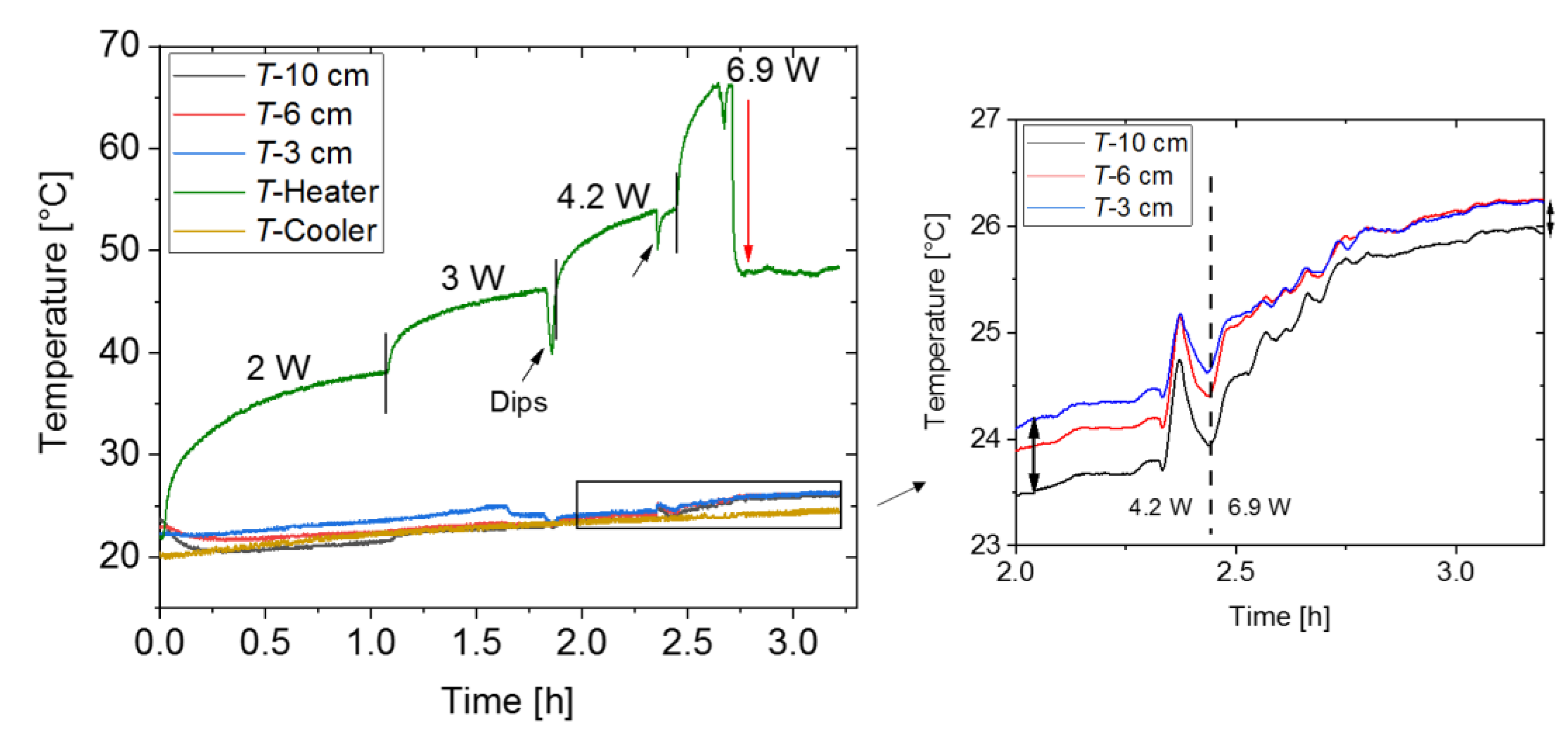
3.2.1. Temperatures vs. Time for Different Heating Powers

Figure 13 and Figure 14 show the relevant temperatures (thermocouple locations see Figure 7) for the different applied heating powers. Since the duration of the whole experiment was long, the experiment was divided into two subsequent experimental sequences. After the first sequence (Figure 13), the heater power was switched off and the heat pipe returned to its original state overnight. Afterwards and during the next day, the second sequence (Figure 14) was carried out.

As can be seen in Figure 13, for the first three temperature levels, the heat pipe operation is severely limited due to a lack of working fluid available at the evaporator. There are occasional dips in heater temperature due to a single liquid drop returning to the evaporator zone. The effect of this is only temporary, as can be seen by the heater temperature quickly returning to its former level.

However, there is a clear change in heat pipe operation as soon as a power level of 6.9 W is applied and a temperature of 66 °C is reached. At first, the temperature increase due to the increased power is stopped abruptly and the temperature stagnates. This is the first indication that large amounts of working fluid in the heat pipe are released abruptly and “switch-like”. Shortly afterwards, there is a quick, drastic and permanent temperature drop from 66 to a continuous temperature plateau at about 48 °C, indicating that there is now a sufficient amount of water available at the evaporator to sustain a permanent fluid circulation and to enable a continuous operation of the heat pipe. The significant reduction of the temperature difference between heater and cooler and, simultaneously, a reduced difference between the temperatures in the adiabatic zone (inset in Figure 13) indicates a significant drop of thermal resistance.

As mentioned above, the second sequence was started on the next day with the heat pipe resting over night without applied thermal power. The sequence as shown in Figure 14 was started with the same power level that was used at the end of the first sequence. In contrast to the first sequence, the applied power was now set from zero directly to 6.9 W and the starting temperatures before this power step were different. Nevertheless, despite these different starting conditions the temperature drop observed during the first sequence could almost exactly be reproduced.

Afterwards, the power was increased stepwise above 6.9 W. Up to the highest applied power of 30 W, no sudden changes in temperature (peaks, dips or thermal runaway) were observed during each power plateau and the difference between the temperatures in the adiabatic zone increased only slightly. This indicates a continuous and steady operation of the heat pipe due to a sufficient amount of working fluid always available at the evaporator.

3.2.2. Comparison to Predictions on Activation Temperature

For comparison of predicted adsorbent loading with the experimentally observed activation temperature in the heat pipe, one has to consider that there is a temperature drop along the borosilicate glass heat pipe wall. The temperature drop can be calculated from the well-known relation for the thermal resistance of a cylinder wall (see for example [28]):

$$R_{th-wall}=\frac{\ln \left(r_a\right)-\ln \left(r_i\right)}{2\cdot {\lambda }_{glass}\cdot \pi \cdot l}$$

(8)

Here, $r_a$ is the heat pipe’s outer radius of 9 mm, $r_i$ is the inner radius of 7.2 mm, ${\lambda }_{glass}$ is the thermal conductivity of borosilicate glass of 1.2 W/(mK) and l is the filling height of the adsorbent of circa 5 cm. Inserting these values in Equation (8) yields a thermal wall resistance of 0.59 K/W and a corresponding wall temperature drop of circa 4 K at a heating power of 6.9 W.

The cooling water temperature around the activation point of the heat pipe was at 24–25 °C, meaning that the temperature at the inner wall of the heat pipe in the condenser zone was at about 29 °C. This corresponds to a water vapor pressure of 4 kPa, as represented by the orange isobar as given in Figure 12.

The isobar predicts an abrupt release of bound water starting at a temperature of approximately from 64 to 66 °C. Correspondingly, as described above, an activation of the heat pipe was experimentally observed at an adsorbent temperature of 62 °C (heater temperature of 66 °C minus the mentioned temperature drop).

In conclusion, the predicted start temperature of abrupt water release from the adsorbent and the heat pipe’s observed activation temperature are in very good agreement and differ only slightly.

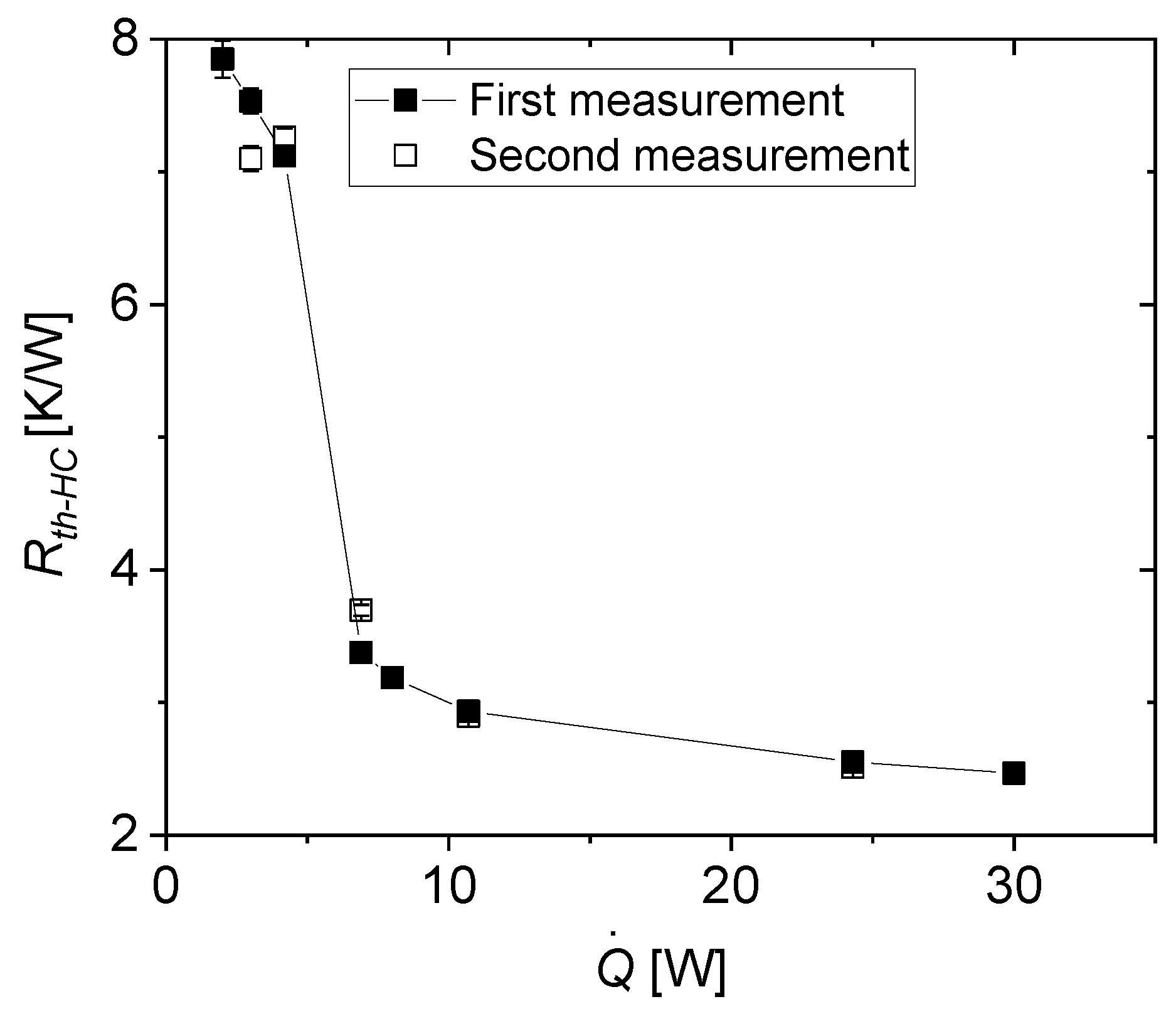
3.2.3. Thermal Resistance

There is a variety of methods to evaluate and visualize the switching effect in heat pipe-based thermal switches. One quite common and intuitive method is to plot applied heating power vs. resulting temperature difference and then use a linear fit to the data points to obtain the thermal conductance (Reference [2], Figure 9) or thermal conductivity [5]. However, the used linear fit corresponds to an averaging over a wide power range that makes it somewhat difficult to see at exactly which power the thermal conductance or conductivity exhibit an evident change, indicating a heat switching effect. Therefore, in this work, we decided to give a separate value of the thermal resistance for each pair of heating power and temperature difference. Two different thermal resistances are used:

• $R_{th-HC }$ as thermal resistance between heater and cooler, where $\mathsf{\Delta }{T}_{HC}$ is the temperature difference between heater (evaporator) and cooler (condenser) at the end of the respective power plateau with heating power $\dot{Q}$:

  $$R_{th-HC}=\frac{\mathsf{\Delta }{T}_{HC}}{\dot{Q}}.$$

  (9)
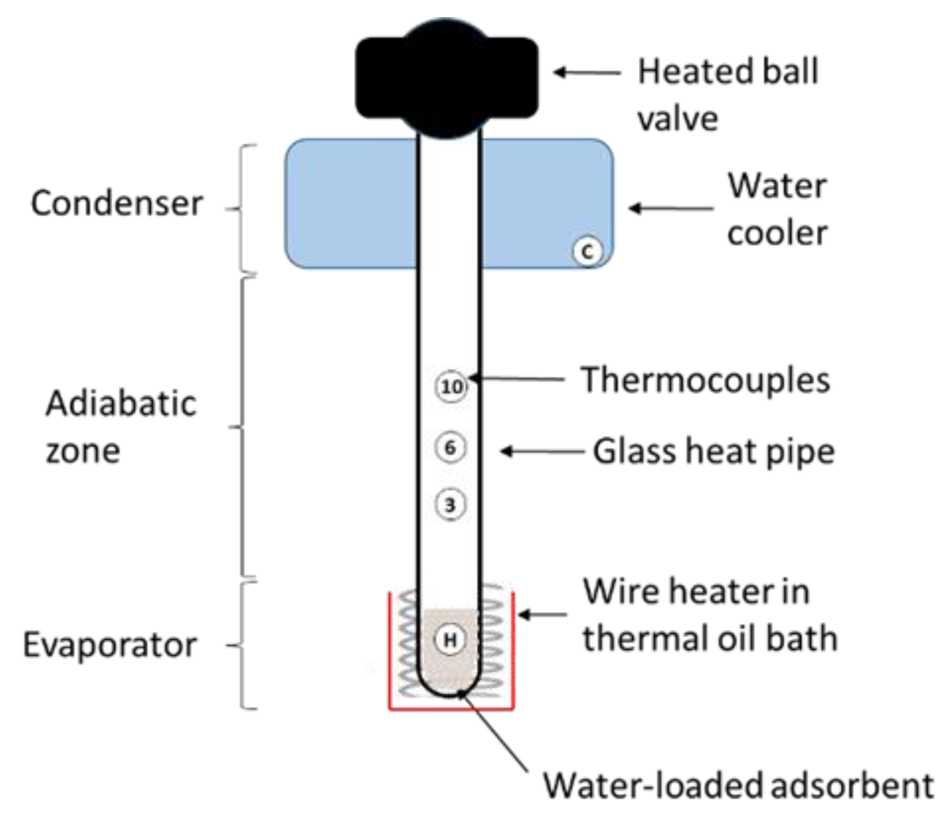
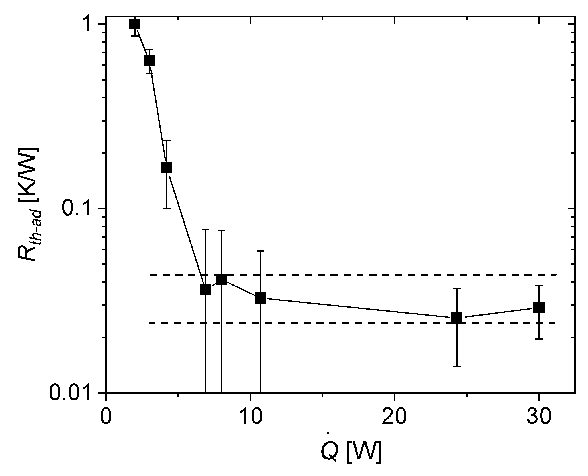
• $R_{th-ad }$ as thermal resistance in the adiabatic zone where $\mathsf{\Delta }{T}_{ad}$ is the temperature difference between the thermocouples located 3 cm and 10 cm above the surface of the thermal oil bath (see Figure 7) at the end of the respective power plateau at heating power $\dot{Q}$:

  $$R_{th-ad}=\frac{\Delta T_{ad}}{\dot{Q} }.$$

  (10)

Figure 15 shows $R_{th-HC }$ versus applied heating power. For powers between 2 and 4.2 W, $R_{th-HC }$ is in a similar region of about 7–8 K/W. In agreement with the observations above (Figure 13 and Figure 14) at 6.9 W, the thermal resistance drops sharply by more than 50% and decreases further for higher heating powers. Altogether, considering thermal resistance gives more evidence that the integration of water-loaded adsorbent in the heat pipe resulted in a clear switching effect, i.e., a strong reduction of the thermal resistance of the heat pipe above defined temperatures. In other words, the heat pipe acts as a heat switch, switching from a less heat-conducting “off”-state to a heat conducting “on”-state.

In order to test the reproducibility of the thermal switching, the measurements were repeated for selected powers around the “switching threshold” at 6.9 W. Between the measurements, the heat pipe was allowed to settle over night without applied heating power. The obtained $R_{th-HC }$ showed a very good agreement to the first measurement sequence.

Figure 16 shows a plot of $R_{th-HC }$ vs. heater temperature. As shown in Figure 13, the temperature at the end of the power plateau of 6.9 W was significantly lower than at the beginning due to the thermal switching effect. Therefore, in addition to the usual $R_{th-HC }$ derived from the temperatures at the end of each power plateau, for 6.9 W additionally $R_{th-HC }$derived from the temperature at the start of this heating power is given.

In addition to the thermal resistance between heater and cooler, $R_{th-HC }$, one can also consider the thermal resistance $R_{th-ad }$in the adiabatic zone of the heat pipe. This thermal resistance represents the thermal resistance of the heat pipe itself more accurately since it does not contain other “parasitic” thermal resistances such as the resistance between heater wire and heat pipe, between heat pipe and cooler etc. Consequently, the thermal switching effect is more clearly evident here (Figure 17). For heating powers below 6.9 W, $R_{th-ad }$is in the range of about 0.2–1 K/W while the heat pipe is in the off-state. At a power level of 6.9 W and above, the heat pipe enters the heat-conducting on-state and $R_{th-ad }$ drops to values that are consistently lower by about one order of magnitude and lie within a narrow range of 0.03–0.04 K/W.

3.2.4. Switching Ratio $r$

The switching ratio $r$ strongly depends on the definition and the methodology used to extract it from the experimental data. As can be seen in the figures above, three regimes can be identified:

• At low power (mostly at 4.2 W and below), the heat pipe is in its non-conducting or off-state.
• Upon increasing the power, the thermal resistance decreases drastically. The drop in thermal conductivity is not perfectly sharp and can extend over more than one power level.
• After the transition to the conducting state, the thermal resistance reaches a relatively constant plateau and does not significantly decrease for higher power levels. Moreover, no significant increase of thermal resistance was observed during the experiment, which means that the heat pipe does not dry out for applied heating powers of at least 30 W.

The numeric value for the switching ratio obtained from heat pipe experiments strongly depends on how it is defined and obtained. As explained in Section 3.2.3, one possible method is to plot applied heating power vs. resulting temperature difference and then use two linear fits to the data points to obtain the thermal conductance or thermal conductivity before and after switching (see for example Reference [2], Figure 9). However, there is often a broad nonlinear transition zone between the on and off state and a certain amount of data points in this zone has to be excluded from the fits. Depending on the amount of data points excluded, the resulting fits may yield different slopes and different results for the thermal resistance and thus also different switching ratios. Therefore, we decided to give multiple switching ratios extracted from the experiment under different definitions:

• $r_{se}$ as ratio of thermal resistances $R_{th-HC }$ and $R_{th-ad}$ obtained at the lowest and highest heating power used in the experiment (2 and 30 W). As can be predicted from Figure 15 and Figure 17, this yields the highest value for the switching ratio.
• $r_{step}$ as ratio of thermal resistances $R_{th-HC }$ and $R_{th-ad}$ at the power level before the observed switching effect takes place (4.2 W), and the power level after switching (6.9 W). This yields a low value for the switching ratio since the transition is not perfectly sharp.
• $r_{av}$ as the ratio of all thermal resistances $R_{th-HC }$and $R_{th-ad}$ averaged before switching (from 2 to 4.2 W) and those averaged after switching (from 6.9 W to 30 W.) This averaged switching ratio probably best represents the overall behavior of the heat pipe as a thermal switch.

The obtained switching ratios according to these definitions are shown in

Table 1. Switching ratios based on different definitions as given in the text above.

UsedRth	${\mathit{r}}_{\mathit{s}\mathit{e}}$	${\mathit{r}}_{\mathit{s}\mathit{t}\mathit{e}\mathit{p}}$	${\mathit{r}}_{\mathit{a}\mathit{v}}$
$R_{th-HC }$	3.2	2.1	2.6
$R_{th-ad }$	35	4.6	18

.

4. Conclusions

In this work, a novel approach for thermal switching using a water-loaded adsorbent in the evaporator of a heat pipe (thermosyphon) is presented. From the results, we conclude that:

• It is possible to predict the “activation temperature” of a heat pipe with integrated adsorbent based on the adsorbent’s isotherm equilibrium data.
• Polanyi’s potential theory can be used in this context to perform the necessary calculations.
• With the presented approach, it is possible to realize a heat switch with averaged thermal switching ratios of 3 and 18 (depending on whether evaporator/condenser or the adiabatic zone are considered).

As the next development step, the setup will be improved:

• The used glass heat pipe demonstrator has its limitations and therefore we are planning to adapt the concept to conventional copper heat pipes and common diameters used in applications (typically around 10 mm).
• The main challenges will be the proper integration of the adsorbent into the heat pipe, determining the appropriate amount of adsorbent and heater position, and ensuring a gravity-independent operation.
• Furthermore, experiments will be carried out to yield defined switching temperatures that are adapted to the individual requirements of the technical application to be addressed (i.e., battery systems, fuel cells etc.).
• Finally, the heat pipe’s transient behavior will be examined in more detail. This means testing the thermal behavior for different holding times at each power level, going back from high temperatures to low temperatures etc.

5. Patents

The concept of realizing a thermal switch based on an adsorption material in a heat pipe was filed for patent (reference EP20180665.0).

References

1. Blumenthal, P.; Raatz, A. Classification of electrocaloric cooling device types. EPL 2016, 115, 17004. [Google Scholar] [CrossRef]
2. Wehmeyer, G.; Yabuki, T.; Monachon, C.; Wu, J.; Dames, C. Thermal diodes, regulators, and switches: Physical mechanisms and potential applications. Appl. Phys. Rev. 2017, 4, 41304. [Google Scholar] [CrossRef] [Green Version]
3. Reay, D.A.; Kew, P.A.; McGlen, R.J. Heat Pipes: Theory, Design and Applications, 6th ed.; Butterworth-Heineman: Oxford, UK, 2013. [Google Scholar]
4. Groll, M.; Munzel, W.D.; Supper, W.; Savage, C.J. Development of a Liquid-Trap Heat Pipe Thermal Diode. J. Spacecr. Rockets 1979, 16, 195–202. [Google Scholar] [CrossRef]
5. Boreyko, J.B.; Zhao, Y.; Chen, C.-H. Planar jumping-drop thermal diodes. Appl. Phys. Lett. 2011, 99, 234105. [Google Scholar] [CrossRef] [Green Version]
6. Tsukamoto, T.; Hirayanagi, T.; Tanaka, S. Micro thermal diode with glass thermal insulation structure embedded in a vapor chamber. J. Micromech. Microeng. 2017, 27, 45001. [Google Scholar] [CrossRef]
7. Benafan, O.; Notardonato, W.U.; Meneghelli, B.J.; Vaidyanathan, R. Design and development of a shape memory alloy activated heat pipe-based thermal switch. Smart Mater. Struct. 2013, 22, 105017. [Google Scholar] [CrossRef]
8. Leriche, M.; Harmand, S.; Lippert, M.; Desmet, B. An experimental and analytical study of a variable conductance heat pipe: Application to vehicle thermal management. Appl. Therm. Eng. 2012, 38, 48–57. [Google Scholar] [CrossRef]
9. Thommes, M.; Kaneko, K.; Neimark, A.V.; Olivier, J.P.; Rodriguez-Reinoso, F.; Rouquerol, J.; Sing, K.S.W. Physisorption of gases, with special reference to the evaluation of surface area and pore size distribution (IUPAC Technical Report). Pure Appl. Chem. 2015, 87, 1051–1069. [Google Scholar] [CrossRef] [Green Version]
10. Sauerbeck, S.; Manoylova, O.; Tissler, A.; Dienersberger, M. Titano-Silico-Alumino-Phosphate. US 2013/0334460 AA, 12 April 2017. [Google Scholar]
11. Freni, A.; Bonaccorsi, L.; Calabrese, L.; Caprì, A.; Frazzica, A.; Sapienza, A. SAPO-34 coated adsorbent heat exchanger for adsorption chillers. Appl. Therm. Eng. 2015, 82, 1–7. [Google Scholar] [CrossRef]
12. Kayal, S.; Baichuan, S.; Saha, B.B. Adsorption characteristics of AQSOA zeolites and water for adsorption chillers. Int. J. Heat Mass Transf. 2016, 92, 1120–1127. [Google Scholar] [CrossRef]
13. Goldsworthy, M.J. Measurements of water vapour sorption isotherms for RD silica gel, AQSOA-Z01, AQSOA-Z02, AQSOA-Z05 and CECA zeolite 3A. Microporous Mesoporous Mater. 2014, 196, 59–67. [Google Scholar] [CrossRef]
14. Kohler, T.; Hinze, M.; Müller, K.; Schwieger, W. Temperature independent description of water adsorption on zeotypes showing a type V adsorption isotherm. Energy 2017, 135, 227–236. [Google Scholar] [CrossRef]
15. Greenspan, L. Humidity fixed points of binary saturated aqueous solutions. J. Res. Natl. Bur. Stand. Sect. A 1977, 81A, 89. [Google Scholar] [CrossRef]
16. Polanyi, M. Section III—Theories of the adsorption of gases. A general survey and some additional remarks. Trans. Faraday Soc. 1932, 28, 316–333. [Google Scholar] [CrossRef]
17. Polanyi, M. Über die Adsorption vom Standpunkt des dritten Waermesatzes. Verh. Dtsch. Phys. Ges 1914, 16, 1012–1016. [Google Scholar]
18. Dubinin, M.M. Theory of the physical adsorption of gases and vapors and adsorption properties of adsorbents of various natures and porous structures. translated version. Russ. Chem. B 1960, 9, 1072–1078. [Google Scholar] [CrossRef]
19. Ruthven, D.M. Principles of Adsorption and Adsorption Processes; Wiley & Sons: New York, NY, USA, 1984; ISBN 0-471-86606-7. [Google Scholar]
20. Langmuir, I. The adsorption of gases on plane surfaces of glass, mica and platinum. J. Am. Chem. Soc. 1918, 40, 1361–1403. [Google Scholar] [CrossRef] [Green Version]
21. Hauer, A. Beurteilung Fester Adsorbentien in Offenen Sorptionssystemen für Energetische Anwendungen. Ph.D. Thesis, Technische Universität Berlin, Berlin, Germany, 2002. [Google Scholar]
22. Semprini, S.; Lehmann, C.; Beckert, S.; Kolditz, O.; Gläser, R.; Kerskes, H.; Nagel, T. Numerical modelling of water sorption isotherms of zeolite 13XBF based on sparse experimental data sets for heat storage applications. Energ. Convers. Manag. 2017, 150, 392–402. [Google Scholar] [CrossRef]
23. Dubinin, M.M.; Astakhov, V.A. Description of Adsorption Equilibria of Vapors on Zeolites over Wide Ranges of Temperature and Pressure. Adv. Chem. 1971, 102, 69–85. [Google Scholar] [CrossRef]
24. Tomás Núnez. Charakterisierung und Bewertung von Adsorbentien für Wärmetranformationsanwendungen. Ph.D. Thesis, Albert-Ludwigs-Universität, Freiburg im Breisgau, Germany, 2001.
25. McKinney, W. Data Structures for Statistical Computing in Python. In Proceedings of the 9th Python in Science Conference, Austin, TX, USA, 28 June–3 July 2010; pp. 56–61. [Google Scholar]
26. Harris, C.R.; Millman, K.J.; van der Walt, S.J.; Gommers, R.; Virtanen, P.; Cournapeau, D.; Wieser, E.; Taylor, J.; Berg, S.; Smith, N.J.; et al. Array programming with NumPy. Nature 2020, 585, 357–362. [Google Scholar] [CrossRef]
27. Hunter, J.D. Matplotlib: A 2D Graphics Environment. Comput. Sci. Eng. 2007, 9, 90–95. [Google Scholar] [CrossRef]
28. Incropera, F.P.; DeWitt, D.P.; Bergman, T.L.; Lavine, A.S. Incropera’s Principles of Heat and Mass Transfer, 1st ed.; John Wiley & Sons Inc.: Hoboken, NJ, USA, 2017; ISBN 9781119382911. [Google Scholar]
Figure 1. Basic concept of thermal heat switch. Below the activation temperature or switching temperature T S , the working fluid is in an adsorbed state and the heat pipe exhibits a high thermal resistance. Above T S , the working fluid is released by desorption. Latent heat transport is enabled, significantly lowering the thermal resistance of the heat pipe.
Energies 14 05130 g001
Figure 2. Classification of physisorption isotherms according to [9].
Energies 14 05130 g002
Figure 3. Connection of isobaric desorption of water from TAPSO-34 and adsorption isotherms of pure TAPSO-34 powder (data taken from Kohler et al. [14]). The amount of desorbed water x   depends on the loading difference of the different isotherms at the same water vapor pressure.
Energies 14 05130 g003
Figure 4. Pre-treatment of the adsorbent at defined humidity.
Energies 14 05130 g004
Figure 5. Schematic of Quantachrome Autosorb iQ surface area analyzer, based on volumetric sorption measurement.
Energies 14 05130 g005
Figure 6. Gravimetric sorption analysis system, Rubotherm IsoSORP series.
Energies 14 05130 g006
Figure 7. Heat pipe demonstrator. Positions of thermocouples are indicated by: H = thermocouple attached to heat pipe wire heater; C = thermocouple immersed in water in water cooler; 10, 6 and 3 = thermocouples attached in the adiabatic zone at 10, 6 and 3 cm above the surface of the thermal oil bath.
Energies 14 05130 g007
Figure 8. Comparison of measured adsorption isotherms with literature data from Kohler [14].
Energies 14 05130 g008
Figure 9. (a) Measured isotherms in W-ϕ-space, adsorption potential according to Polanyi. (b) Measured isotherms in W-ϕ-space, adsorption potential according to Kohler.
Energies 14 05130 g009
Figure 10. Description of the characteristic curve of granular TAPSO-34 by a straight line in the range of low adsorption potential and a third-order fractional polynomial in the range of high adsorption potential.
Energies 14 05130 g010
Figure 11. Adsorption isotherms calculated from the potential theory using the characteristic curve from Figure 10 in comparison with the measured isotherms.
Energies 14 05130 g011
Figure 12. Calculated adsorption isobars in comparison to measured adsorption isobars at adsorptive water vapor pressures of 3.17 and 4.01 kPa, which corresponds to a condenser temperature of the heat pipe of 25 and 29 °C, respectively.
Energies 14 05130 g012
Figure 13. First sequence of temperatures measured along heat pipe vs. time for different heating powers (temperature measurement locations as defined in Figure 7). (Left image) All temperatures including heater and cooler temperature. Vertical black lines indicate the beginning and end of each power plateau, respectively. The red arrow indicates a significant temperature drop associated with the abrupt release of the working fluid water. (Right image) Inset with temperatures in adiabatic zone only.
Energies 14 05130 g013
Figure 14. Second sequence of temperatures measured along heat pipe vs. time for different heating powers (temperature measurement locations as defined in Figure 7).
Energies 14 05130 g014
Figure 15. R t h H C   versus heating power (full squares). The measurements were repeated to evaluate the reproducibility of the thermal switching effect (empty squares). Lines are given as eye guides.
Energies 14 05130 g015
Figure 16. R t h H C   versus heater temperature.
Energies 14 05130 g016
Figure 17. R t h a d   versus heating power with logarithmic y-axis. Solid lines: eye guide. Dashed lines: narrow range of values for R t h a d   when the heat pipe is in the on-state.
Energies 14 05130 g017