Hydrodynamic Modeling of Oil–Water Stratified Smooth Two-Phase Turbulent Flow in Horizontal Circular Pipes

Abstract

In the petrochemical industry, multiphase flow, including oil–water two-phase stratified laminar flow, is more common and can be easily obtained through mathematical analysis. However, there is limited mathematical analytical model for the simulation of oil–water flow under turbulent flow. This paper introduces a two-dimensional (2D) numerical simulation method to investigate the pressure gradient, flow field, and oil–water interface height of a pipeline cross-section of horizontal tube in an oil–water stratified smooth flow. Three Reynolds average N–S equation models ($k-\epsilon$, $k-\omega$, SST $k-\omega$) are involved to simulate oil–water stratified smooth flow according to the finite volume method. The pressure gradient and oil–water interface height can be computed according to the given volume flow rate using the iteration method. The predicted result of oil–water interface height and velocity profile by the model fit well with several published experimental data, except that there is a large error in pressure gradient. The SST $k-\omega$ turbulence model appears higher accuracy for simulating oil–water two-phase stratified flow in a horizontal pipe.

1. Introduction

In petroleum transportation, the oil–water two-phase flow is very economic and common technique [1]. The pressure gradient, oil–water interface height, and velocity field are important factors to design the pipe [2] and separator [3]. Pressure gradient is an important basis for designing the wall thickness of pipelines and pressure vessels. Oil–water interface height is used to design the carrying capacity of downstream facilities. Accurate prediction of the velocity field of the pipeline cross-section is helpful for controlling flow assurance issues, such as wax deposition [4], hydrate formation [5], pipeline corrosion [6], etc. Therefore, in order to optimize piping design and equipment operating parameters, two-phase flow has been widely studied. There are multiple flow patterns in oil–water pipe flow, such as stratified flow, dispersed flow, and annular flow, for different fluid properties and flow conditions. Among the above flow patterns, stratified flow is the common. The calculation of oil–water interface height, pressure gradient, and velocity field involve solving the pipeline two-phase hydrodynamic model.

In the past, most scholars used the one-dimensional two-fluid model of gas–liquid two-phase flow [7,8] to study oil and water, and improved the accuracy of the model by modifying the interface configuration function, and the shear stress model of wall and oil–water interface [9]. Ullmann [10] improved the two-fluid model to consider the contraction of the shear stress at the wall and oil–water interphase. The model was verified against experiments in the literature and provided the pipe flow of laminar flow with an accurate solution. Later, Ullmann and Brauner [11] considered the influence of interfacial waves on interfacial shear and developed an experience correction formula for wavy stratified flow. Awad and Butt [12] built a semitheoretical method to predict the pressure gradient caused by friction by establishing a dual pressure model. Rodriguez and Baldani [13] employed the interface wave amplitude as the interface friction coefficient to establish a new closure relationship, considering that the interface between the oil and water phases is an arc of constant curvature in large-diameter pipe (26 mm). Edomwonyi-Otu [14] measured the interface wave amplitude of low-viscosity oil–water flow on a medium pipe diameter (14 mm), corrected the interface roughness to improve the interface shear stress model, and modified the interface configuration and roughness coupled into the one-dimensional two-fluid model. The accuracy of the hydrodynamic model was improved. However, these models determine only one-dimensional steady-state for no cross-section information.

Recently, there have been a number of works considering phase interface tracking [15,16] and accuracy of variables computed [17,18] in this area, including some recent research on mesh adaptivity for multiphase flow applications [19,20,21,22]. López-Herrera [21] proposed an adaptive numerical solver for the investigation of 2D two-phase flow with VOF method. Liu [22] established an adaptive coupled VOF and level set method based on unstructured grids to study incompressible two-phase flow. The interface tracking method can describe the shape of the interface well, and adaptive mesh can refine the interface and reduce the number of grids compared to fixed mesh. However, traditional 3D adaptive mesh coupled with the interface tracking method still needs a large number of grids and is not suitable for steady-state calculation.

In order to predict the flow field of steady-state multiphase flow, the use of computational fluid method that does not require high computational complexity has attracted the attention of scholars. Issa [23] built a coupled standard $k-\epsilon$ two-equation model to calculate steady and fully developed gas–liquid two-phase stratified turbulence flow, and used a bipolar coordinate system to describe the pipe geometry. This model can calculate gas–liquid interface height, pressure gradient, and velocity field of liquid and gas phase. Newton [24] employed a low Reynolds number $k-\epsilon$, two-equation turbulence model to predict the gas–liquid stratified flow in a pipe with a diameter of 50 mm. A damping function was applied to the wall, and the numerical results were in good agreement with the experimental results. De Sampaio [25] utilized the finite element method coupled with $k-\omega$ turbulence model to predict gas–liquid two-phase pipe flow. Duan [26,27,28,29] established a two-dimensional wax deposition model to predict the wax deposition thickness of petroleum pipelines, coupled with the energy equation and $k-\epsilon$ turbulence model. He [30] used the large eddy simulation turbulence model and coupled the phase change model to investigate the mass transfer process between gas and liquid phases, as well as the temperature field and flow field distribution of the pipe cross section.

The above calculation algorithms are all used for the numerical simulation of gas–liquid two-phase flow. Recently, Maklakov [31] established a mathematical model of the pipe cross sectional configuration of the oil–water stratified laminar flow through mathematical analysis, considering the pipeline inclination, capillary force, and other factors, which can predict the velocity field of pipe cross section. However, this model is only suitable for oil–water laminar flow conditions. Later, Li [32] firstly applied the two-dimensional flow model of gas–liquid to oil–water liquid–liquid flow to research the non-Newtonian characteristics of oil–water stratified flow on horizontal pipes. However, compared with the gas–liquid two-phase flow, the oil–water two-phase flow has significant differences, mainly due to the small oil–water density difference, the small viscosity difference, and the small velocity difference between the two phases. In fact, the shear stress between the oil–water two-phase interface is stronger than the gas–liquid two-phase for stratified flow.

The primary intention of this work is to investigate oil–water two-phase pipe flow through establishing a steady-state 2D oil–water two-phase stratified flow model in a bipolar coordinate system, where three turbulence models ($k-\epsilon$, $k-\omega$, SST $k-\omega$) are utilized to simulate the turbulence flow. Then, the finite volume method is used to discrete the model and an adaptive mesh method is utilized to track the oil and water interface. After the convergence of velocity and turbulence field, the total mass flow conservation is used to adjust the pressure gradient and oil–water interface height. In addition, pressure gradient, oil–water interface height, and velocity field are compared with experimental data to validate the presented hydraulic model under three different turbulence models.

2. Materials and Methods

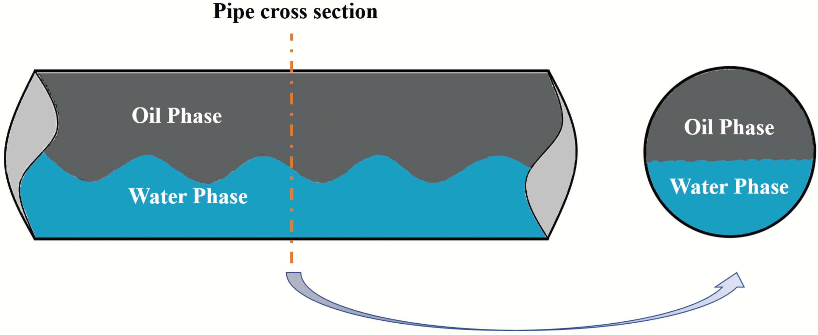
2.1. Problem Description and Model Assumption

In this section, a 2D isothermal horizontal pipe oil–water stratified flow model is demonstrated. The governing formulas are composed of mass conservation equations, momentum conservation equations, and turbulence models. Oil transportation is usually carried out by mixing oil and water as shown in Figure 1. In the later stage of oil exploitation, oil transportation is mostly in a stable two-phase stratified flow of oil and water in the pipeline. Crude oil contains colloidal asphaltenes and other impurities, which will affect the flow assurance issue, and pressure gradient, oil–water interface height, and velocity field of the pipe cross section are important parameters for oil–water flow assurance. Therefore, it is important to establish a steady hydraulic model of oil–water two-phase pipe flow.

Assumptions are made as follows: (1) The oil and water are in a smooth and steady stratified flow, and there is no emulsified layer at the interface; (2) the oil phase is homogeneous and does not have non-Newtonian characteristics; (3) the influences of heat transfer are negligible; (4) the flow of oil and water is fully developed at steady-state.

2.2. Governing Equation

2.2.1. Mass Conservation Equation

For simplified calculation, the model’s premise is that the emulsification between oil and water, non-Newtonian characteristics, and thermal transmission are not considered. As the oil and water are incompressible, the total flow rate of the oil and water phases remains unchanged on each section of the pipe axis. Therefore, the mass conservation equation can be obtained by

$$Q_{}=Q_{inlet,o}+Q_{inlet,w}={\int }_{A_{oil}}{w}_{oil}dA+{\int }_{A_{water}}{w}_{water}dA$$

(1)

where $w_{oil}$ and $w_{water}$ are the axial velocities of the oil and water phases, m/s. $A_{oil}$ and $A_{water}$ are the circulation areas of the oil and water phases, m. $Q_{oil}$ and $Q_{water}$ are volume flow rates at the inlet of the oil and water phases, m${}^3$/s.

2.2.2. Momentum Conservation Equation

The Navier–Stokes formula of fully developed oil–water stratified pipe flow along the axial direction of the pipeline is depicted in Equation (2), which assumes that the oil–water two-phase flow is incompressible.

$$\frac{\partial }{\partial x}\left({\mu }_e\frac{\partial w}{\partial x}\right)+\frac{\partial }{\partial y}\left({\mu }_e\frac{\partial w}{\partial y}\right)=\frac{dp}{dz}$$

(2)

where ${\mu }_e$ is the effective viscosity coefficient of the oil or water phase, ${\mu }_e={\mu }_m+\gamma {\mu }_t$, and N·/m${}^2$. $\frac{dp}{dz}$ is the flow pressure gradient, Pa/m. A single-pressure model is used to calculate the momentum conservation equation.

2.2.3. Turbulence Model

Oil–water pipeline flow is often turbulent, and the characteristics of turbulence are more complicated than laminar flow. At present, the commonly used turbulence models are large eddy simulation and Reynolds average. Compared with the Reynolds time average, the large eddy simulation requires extensive calculation and significant time. Hence, for quickly obtaining the oil–water flow field information on the cross section of the pipeline, three different Reynolds average models ($k-\epsilon$, $k-\omega$, SST $k-\omega$) are adopted in this study. The governing equations for the $k-\epsilon$ model [33] are as follows:

$$\frac{\partial }{\partial x}\left[\left(\mu +\frac{{\mu }_t}{{\sigma }_k}\right)\frac{\partial k}{\partial x}\right]+\frac{\partial }{\partial y}\left[\left(\mu +\frac{{\mu }_t}{{\sigma }_k}\right)\frac{\partial k}{\partial y}\right]+{\mu }_t\left[{\left(\frac{\partial w}{\partial x}\right)}^2+{\left(\frac{\partial w}{\partial y}\right)}^2\right]-\rho \epsilon =0$$

(3)

$$\frac{\partial }{\partial x}\left[\left(\mu +\frac{{\mu }_t}{{\sigma }_{\epsilon }}\right)\frac{\partial \epsilon }{\partial x}\right]+\frac{\partial }{\partial y}\left[\left(\mu +\frac{{\mu }_t}{{\sigma }_{\epsilon }}\right)\frac{\partial \epsilon }{\partial y}\right]+C_{\epsilon 1}{\mu }_t\left[{\left(\frac{\partial w}{\partial x}\right)}^2+{\left(\frac{\partial w}{\partial y}\right)}^2\right]\frac{\epsilon }{k}-\rho C_{\epsilon 2}\frac{{\epsilon }^2}{k}=0$$

(4)

$${\mu }_t=\rho C_u\frac{k^2}{\epsilon }$$

(5)

where the closure coefficients are given by $C_u=0.09$, $C_{\epsilon 1}=1.44$, $C_{\epsilon 2}=1.92$, ${\sigma }_k=1.0$, and ${\sigma }_{\epsilon }=1.3$. The governing equations for the $k-\omega$ model [34] are as follows:

$$\frac{\partial }{\partial x}\left[\left(\mu +\frac{{\mu }_t}{{\sigma }_k}\right)\frac{\partial k}{\partial x}\right]+\frac{\partial }{\partial y}\left[\left(\mu +\frac{{\mu }_t}{{\sigma }_k}\right)\frac{\partial k}{\partial y}\right]+{\mu }_t\left[{\left(\frac{\partial w}{\partial x}\right)}^2+{\left(\frac{\partial w}{\partial y}\right)}^2\right]-\rho {\beta }^{\ast }\omega k=0$$

(6)

$$\frac{\partial }{\partial x}\left[\left(\mu +\frac{{\mu }_t}{{\sigma }_{\omega }}\right)\frac{\partial w}{\partial x}\right]+\frac{\partial }{\partial y}\left[\left(\mu +\frac{{\mu }_t}{{\sigma }_{\omega }}\right)\frac{\partial w}{\partial y}\right]+\alpha \frac{\omega }{k}{\mu }_t\left[{\left(\frac{\partial w}{\partial x}\right)}^2+{\left(\frac{\partial w}{\partial y}\right)}^2\right]-\rho \beta {\omega }^2=0$$

(7)

$${\mu }_t=\frac{\rho k}{\omega }$$

(8)

where ${\mu }_t$ is the dynamic eddy viscosity, $\mathrm{N}·/{\mathrm{m}}^2$; $\rho$ is the density, m${}^3$/s; and the closure coefficients are given as $\alpha =5/9$, $\beta =0.075$, ${\beta }^{\ast }=0.09$, and ${\sigma }_k={\sigma }_{\omega }=2$. The governing equations for the SST $k-\omega$ model are as follows:

$$\frac{\partial }{\partial x}\left[\left(\mu +{\sigma }_k{\mu }_t\right)\frac{\partial k}{\partial x}\right]+\frac{\partial }{\partial y}\left[\left(\mu +{\sigma }_k{\mu }_t\right)\frac{\partial k}{\partial y}\right]+P_k-\rho {\beta }^{\ast }\omega k=0$$

(9)

$$\begin{array}{cc}\hfill & \frac{\partial }{\partial x}\left[\left(\mu +{\sigma }_{\omega }{\mu }_t\right)\frac{\partial \omega }{\partial x}\right]+\frac{\partial }{\partial y}\left[\left(\mu +{\sigma }_{\omega }{\mu }_t\right)\frac{\partial \omega }{\partial y}\right]+\alpha \rho S^2-\beta \rho {\omega }^2\hfill \\ \hfill & +2(1-F_1){\sigma }_{w2}\rho \frac{1}{\omega }\left(\frac{\partial k}{\partial x}\frac{\partial \omega }{\partial x}+\frac{\partial k}{\partial y}\frac{\partial \omega }{\partial y}\right)=0\hfill \end{array}$$

(10)

$${\mu }_t=\frac{a_{1}k\rho }{max(a_1\omega ,S{F}_2)}$$

(11)

where $S=\sqrt{2S_{ij}{S}_{ij}}$ is the modulus of the mean rate-of-strain tensor and $P_k$ is a limited production term given by the following equation:

$$P_k=min\left({\tau }_{ij}\frac{\partial U_i}{\partial x_j},10{\beta }^{\ast }\rho k\omega \right)$$

(12)

$F_1$ and $F_2$ are blending functions defined by

$$F_1=tanh\left(min{\left[max\left(\frac{500\mu }{\rho \omega y^2},\frac{\sqrt{k}}{{\beta }^{\ast }\omega y}\right),\frac{4\rho {\sigma }_{\omega 2}k}{C{D}_{k\omega }{y}^2}\right]}^4\right)$$

(13)

$$F_2=tanh\left[{\left[max\left(\frac{2\sqrt{k}}{{\beta }^{\ast }\omega y},\frac{500\mu }{\rho \omega y^2}\right)\right]}^2\right]$$

(14)

and

$$C{D}_{k\omega }=max\left(2\rho {\sigma }_{\omega 2}\frac{1}{\omega }\frac{\partial k}{\partial x_i}\frac{\partial \omega }{\partial x_i},{10}^{-10}\right)$$

(15)

The closure coefficient of the SST $k-\omega$ model [35] is obtained by blending those of the $k-\omega$ model, denoted by ${\varphi }_1$, and the standard $k-\epsilon$ model, denoted by ${\varphi }_2$, via the relationship $\varphi ={\varphi }_1{F}_1+{\varphi }_2(1-F_2)$. The coefficients are given by $a_1=5/9$, $a_2=0.44$, ${\beta }^{\ast }=9/100$, ${\beta }_1=3/40$, ${\beta }_2=0.0828$, ${\sigma }_{k1}=0.85$, ${\sigma }_{k2}=1$, ${\sigma }_{\omega 1}=0.5$, and ${\sigma }_{\omega 2}=0.856$.

2.3. Boundary Conditions

On the pipe wall, the nonslip boundary condition is for velocity, turbulent kinetic energy, and eddy viscosity.

$$w_{wall}=k_{wall}={\left({\mu }_t\right)}_{wall}=0$$

(16)

When the Reynolds number is low, the turbulence model can capture the damping effect near the wall. If the Reynolds number exceeds a specific value, the thickness of the viscous sublayer of the boundary layer will become thinner, resulting in a small number of grid points, making it difficult to obtain the results. The wall function [36,37] is employed to avoid the problem. The energy dissipation rate of the point near the wall in the $k-\epsilon$ equation is described as follows:

$${\epsilon }_C=\frac{{C_u}^{0.75}{k}^{1.5}}{K_{karman}d}$$

(17)

The specific energy dissipation rate in the $k-\omega$ equation at the boundary is given by

$${\omega }_C=\frac{\sqrt{k}}{{C_u}^{0.25}{K}_{karman}d}$$

(18)

The SST $k-\omega$ equation combines two specific energy dissipation rates to obtain the near-wall value.

$${\omega }_C={\left[{\omega }_{vis}^2+{\omega }_{log}^2\right]}^{0.5}$$

(19)

where

$${\omega }_{vis}=\frac{6\mu }{\rho {\beta }_1{d}^2}{\omega }_{log}=\frac{\sqrt{k}}{{C_u}^{0.25}{K}_{karman}d}$$

3. Numerical Method

3.1. Governing Equations Discretization

The governing equation is discretized by finite volume in the bipolar coordinate system, and a nonuniformly distributed grid is used in the calculation domain [a, b] and [c, d]. The diffusion term is discretized using the central difference scheme.

$$\frac{1}{l_{\eta }{l}_{\xi }}\frac{\partial }{\partial \eta }\left({\Gamma }_{\varphi }\frac{\partial \varphi }{\partial \eta }\right)+\frac{1}{l_{\eta }{l}_{\xi }}\frac{\partial }{\partial \xi }\left({\Gamma }_{\varphi }\frac{\partial \varphi }{\partial \xi }\right)=S_{\varphi }$$

(20)

The equation form after sorting the discretization is

$$a_P{\varphi }_P+a_E{\varphi }_E+a_W{\varphi }_W+a_N{\varphi }_N+a_S{\varphi }_S=b$$

(21)

where

$$a_E=-{\left({\Gamma }_{\varphi }\frac{\Delta \eta }{\delta \xi }\right)}_e{a}_W=-{\left({\Gamma }_{\varphi }\frac{\Delta \eta }{\delta \xi }\right)}_w$$

$$a_N=-{\left({\Gamma }_{\varphi }\frac{\Delta \xi }{\delta \eta }\right)}_n{a}_S=-{\left({\Gamma }_{\varphi }\frac{\Delta \xi }{\delta \eta }\right)}_s$$

The coefficient $a_p$ is given by

$$a_P=-a_E-a_W-a_N-a_S$$

(22)

The Cartesian coordinate system and the bipolar coordinate system have the following coordinate transformation relationship:

$$x=a\frac{sinh\eta }{cosh\eta -cos\xi }y=a\frac{sin\xi }{cosh\eta -cos\xi }$$

where $\xi$ and $\eta$ are the coordinates of point P in bipolar coordinates. The scalar factor of the bipolar coordinate is given by

$$l_{\xi }=l_{\eta }=\frac{a}{cosh\eta -cos\xi }$$

(23)

with

$$a=\frac{d}{2}\times sin\left({\theta }_1\right)$$

(24)

A bipolar coordinate system is introduced to simulate the two-phase noncircular and irregular regions in the stratified flow more accurately (Figure 2). Through bipolar coordinate transformation, the oil–water stratified pipe flow zone in Cartesian coordinates is transformed into a regular rectangular calculation zone in bipolar coordinates. The calculation zone of the oil phase is ${\theta }_1<\xi <{\theta }_2$, $-\infty <\eta <\infty$. The calculation zone of the water phase is ${\theta }_2<\xi <\pi +{\theta }_1$, $-\infty <\eta <\infty$. In numerical computation, the value of $\eta$ must be an exact value; Newton and Behnia [24] suggested ${\eta }_{max}=6$.

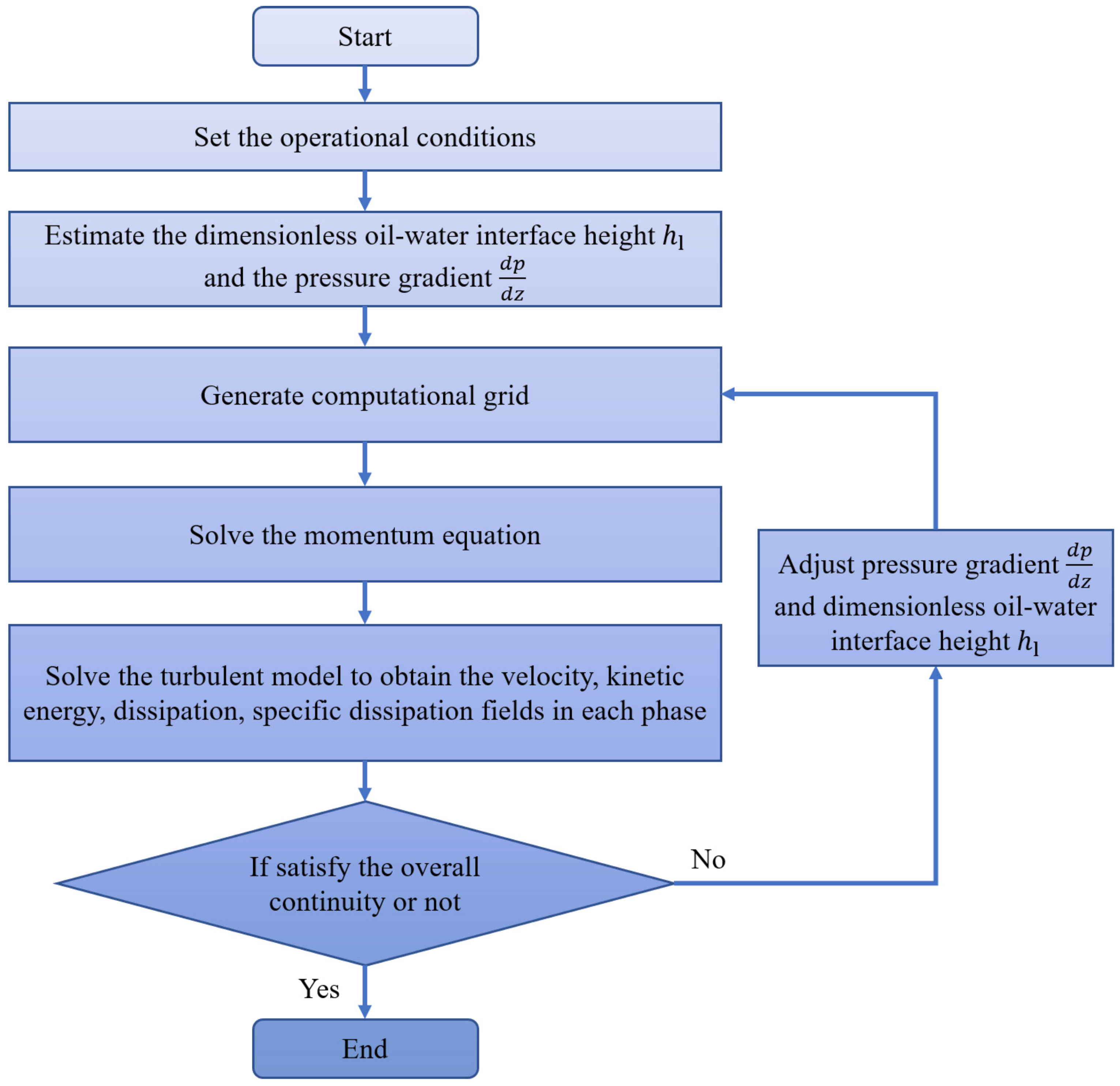
3.2. Solution Methodology

It is necessary to calculate pressure gradient and oil–water interface height to make the velocity field of pipe cross section match the given volume flow. The pressure gradient affects the solution of the momentum equation, and the height of the oil–water interface controls the generation of the adaptive mesh. As shown in Figure 3, the hydrodynamics model is nonlinear. Hence, an iterative solution is required to obtain the pressure gradient, the oil–water interface height, and the velocity field of the pipe cross section that satisfies the mass conservation equation.

The solution of the model is depicted in the flow chart of Figure 3. First, we set the boundary conditions; then, we estimate the oil–water interface height and pressure gradient, and divide the calculation grid. After the grid is divided, the momentum equation and turbulence model can be solved. Thus, the velocity, kinetic energy, and specific energy dissipation region of each phase can be obtained. If the results meet the mass conservation conditions, the calculation ends; otherwise, the oil–water interface height and pressure drop gradient are adjusted, and the calculation continues. Next, we obtain the pressure gradient $dp/dz$ and dimensionless oil–water interface height $h_l$, which is the ratio of the height of the oil–water interface to the pipe diameter. The first is obtained by external iteration calculation, which adopts the Newton–Raphson method to change $dp/dz$ and $h_l$ to satisfy the mass conservation equation. Therefore, we can obtain the oil and water two-phase continuity equations as follows:

$$F(m,n)=Q_w-\underset{A_w}{\int }{w}_{w}dA=0G(m,n)=Q_o-\underset{A_o}{\int }{w}_{o}dA=0$$

(25)

Subsequently, $m=dp/dz$ and $n=h_l$ are introduced to simplify notation. The Newton–Raphson iteration method is applied to calculate the solution of the nonlinear equations represented by Equation (25). The next approximate value is calculated by

$$m^{k+1}=m^k+\frac{{\left(G\frac{\partial F}{\partial n}-F\frac{\partial G}{\partial n}\right)}^k}{{\left(\frac{\partial F}{\partial m}\frac{\partial G}{\partial n}-\frac{\partial G}{\partial m}\frac{\partial F}{\partial n}\right)}^k}{n}^{k+1}=n^k+\frac{{\left(F\frac{\partial G}{\partial m}-G\frac{\partial F}{\partial m}\right)}^k}{{\left(\frac{\partial F}{\partial m}\frac{\partial G}{\partial n}-\frac{\partial G}{\partial m}\frac{\partial F}{\partial n}\right)}^k}$$

(26)

Based on the analysis of Equation (26), the calculation process is iterative. Consequently, it is critical to set the error range reasonably to solve the equation, including the convergence speed, accuracy, calculation results, and so on. When the continuity equation satisfies a specific error range, a reasonable calculation result is obtained.

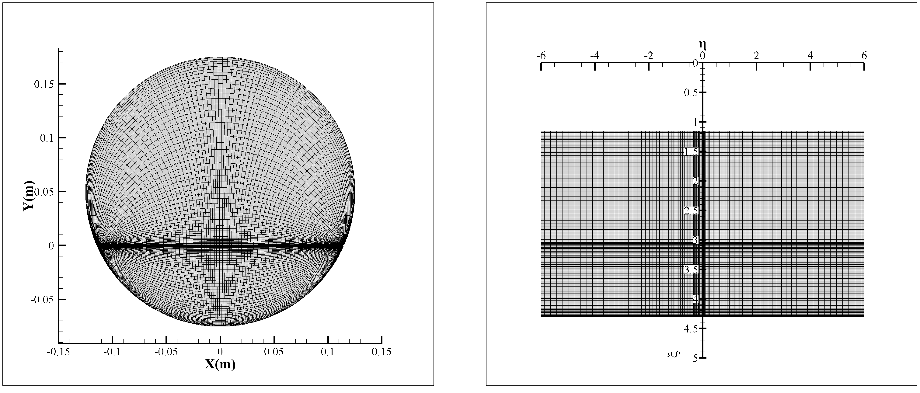
3.3. Grid-Independence Solution

The governing equations are solved on the structure grid, and there is local refinement at the oil–water interface and pipe wall. In order to eliminate the influence of the grid on numerical results, it is necessary to test the grid independence. Through experimentation, Yusuf [38] observed that the oil–water two-phase flow was stratified flow in a 25.4 mm acrylic pipe, when the water superficial velocity is 0.318 m/s and the oil superficial velocity is 0.14 m/s. As shown in Figure 4 and

Table 1. Compare the effect of the number of grids on the pressure gradient $\nabla p$ and dimensionless oil–water interface height $h_l$ for different turbulence models.

Turbulence Model	Grid Set	$\mathit{\nabla }\mathit{p}$ (Pa/m)	Relevate  Change %	${\mathit{h}}_{\mathit{l}}$	Relevate Change %
$k-\epsilon$	20 × 20	218.74	-	0.5533	-
	50 × 50	235.15	7.50	0.5597	1.15
	80 × 80	239.49	1.85	0.5608	0.20
	100 × 100	241.15	0.69	0.5612	0.07
$k-\omega$	20 × 20	211.55	-	0.5608	-
	50 × 50	218.99	3.52	0.5683	1.34
	80 × 80	218.70	0.13	0.5693	0.18
	100 × 100	218.29	0.19	0.5696	0.05
SST$k-\omega$	20 × 20	199.00	-	0.5683	-
	50 × 50	214.24	7.66	0.5723	0.71
	80 × 80	217.00	1.29	0.5723	0.01
	100 × 100	218.57	0.72	0.5726	0.06

, the velocity distribution at vertical centerline on the cross section, pressure gradient, and dimensionless oil–water interface height are calculated and compared by using the proposed algorithm in Yusuf experiments under four sets of grid.

It can be seen from Figure 4 that the velocity distribution under different grid sets has a consistent distribution. However, as shown in Table 1, there are obvious differences in pressure gradient and dimensionless oil–water interface height from 20 × 20 to 50 × 50 mesh. Pressure gradient and dimensionless oil–water interface height only changed by about 1%, when the grid changes from 50 × 50 to 80 × 80, and from 80 × 80 to 100 × 100. Therefore, in this paper, the 80 × 80 mesh is selected to simulate all the cases.

4. Results and Discussion

The model must only input the pipe diameter d, physical properties, and volume flow rates of oil and water phases. Then, the axial pressure gradient, dimensionless oil–water interface height, and velocity and turbulence field of the pipe cross section can be calculated. This section is divided into three subsections. The first subsection validates the turbulence model under a single-phase flow scenario. The second subsection presents the calculation results of the pressure gradient of the two-phase flow and compares them with the experimental values. The last subsection validates the flow field and interface height of the pipe cross section.

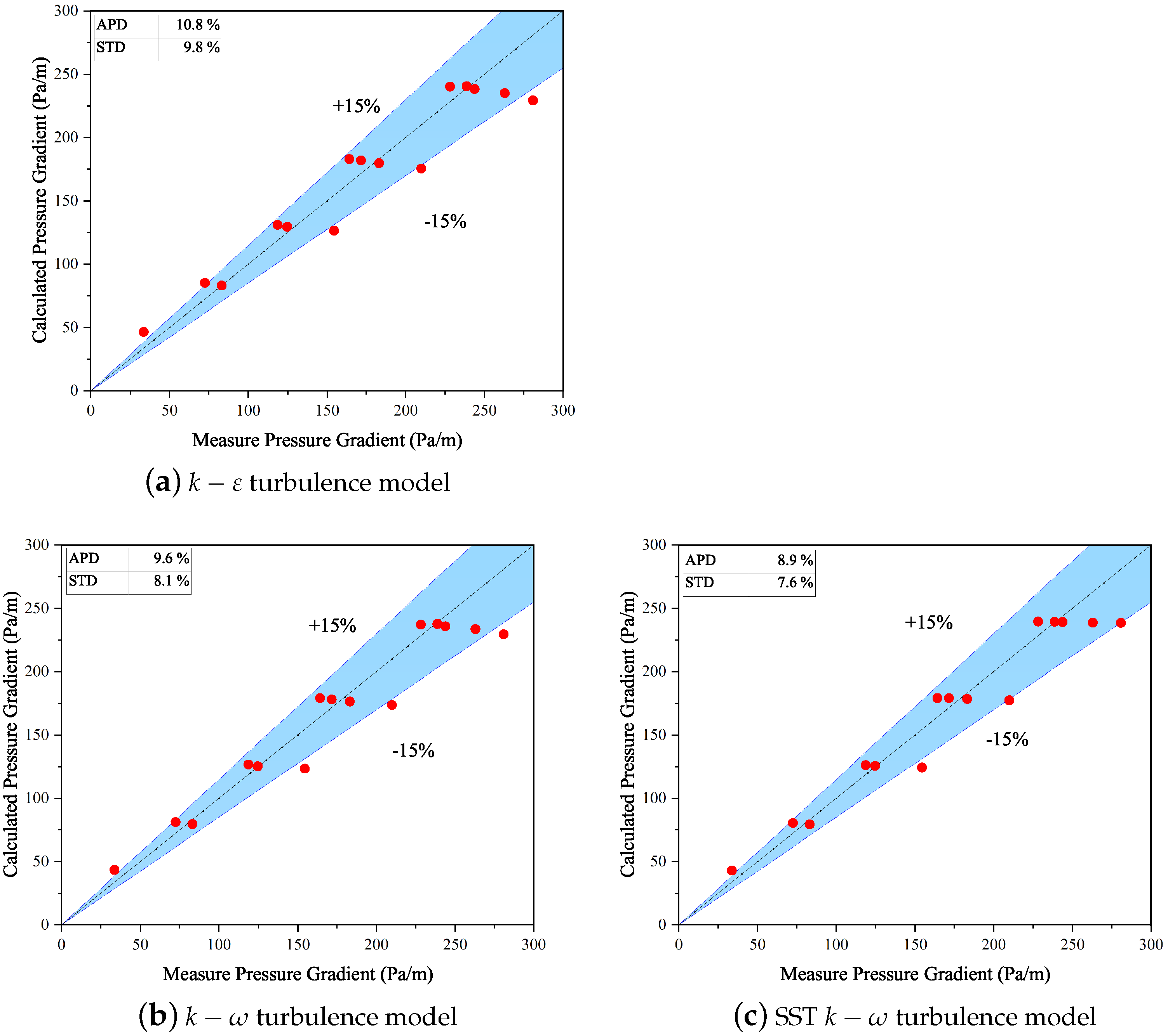
4.1. Turbulence Model Validation

Here, we simulate oil–water two-phase turbulence, and verify the reliability of the algorithm and turbulence model. First of all, a different Reynolds single-phase flow hydraulic calculation is utilized to validate the turbulence models. The calculation result of the Darcy formula was adopted to validate turbulence models. Then, the test includes distributing the identical fluid properties and volume flow rates for both phases. Different flow models were used at different flow regimes, such as laminar and turbulence.

As shown in Figure 5, the pressure gradient of single-phase pipe flow is given under different models. When the turbulence model is coupled, the pressure gradient obtained by the numerical calculation algorithm are completely consistent with the theoretical formula under laminar flow conditions. Then, for the prediction of turbulence in single-phase flow through coupled turbulence models, the calculation outcomes match well with expected values from the Darcy formula, but the pressure gradient was underestimated at a high Reynolds number. Thus, it can be proved that the turbulence models have sufficient accuracy and the algorithm can obtain the correct pressure gradient based on the single-phase flow test.

4.2. Calculation of Two-Phase Flow Pressure Gradient

Before the flow field of the pipe cross section is investigated, the two-phase pressure gradients under different oil–water flow rates with different turbulence models need to be verified. Angeli [39] researched the oil–water two-phase stratified flow in a pipe with an inner diameter of 24.3 mm and length of 9.7 m. The experimental results illustrate that when the mixing velocity is less than or equal to 0.6 m/s, the two-phase flow pattern in the acrylic pipe is stratified flow. Therefore, the superficial velocities of the two phases are chosen to be between 0.11 and 0.55 m/s to satisfy the stratified flow pattern of oil–water two-phase flows. Fifteen experimental data points are applied to confirm the accuracy of the models.

Figure 6 and

Table 2. Comparison of pressure gradient between model predictions and experimental measurements.

No	${\mathit{U}}_{\mathbf{Soil}}$ (m/s)	${\mathit{U}}_{\mathbf{Swater}}$ (m/s)	Exp Data (Pa/m)	$\mathit{k}-\mathit{\epsilon }$		$\mathit{k}-\mathit{\omega }$		SST $\mathit{k}-\mathit{\omega }$
				Values (Pa/m)	Relative Error (%)	Values (Pa/m)	Relative Error (%)	Values (Pa/m)	Relative Error (%)
1	0.11	0.11	33.52	46.51	38.75	43.38	29.43	42.95	28.14
2	0.22	0.11	72.30	85.24	17.89	81.07	12.13	80.50	11.35
3	0.11	0.22	83.06	83.25	0.23	79.70	−4.05	79.40	−4.40
4	0.22	0.22	124.67	129.54	3.90	125.33	0.53	125.65	0.79
5	0.33	0.11	118.54	131.04	10.54	126.61	6.80	126.06	6.35
6	0.33	0.22	171.57	182.07	6.12	178.06	3.78	179.17	4.43
7	0.11	0.33	154.47	126.55	−18.08	123.48	−20.06	124.23	−19.58
8	0.22	0.33	183.02	179.73	−1.80	176.42	−3.60	178.40	−2.53
9	0.33	0.33	243.80	238.44	−2.20	235.85	−3.26	239.30	−1.85
10	0.44	0.11	164.16	183.02	11.49	179.04	9.06	179.12	9.11
11	0.44	0.22	228.24	240.30	5.29	237.24	3.94	239.61	4.98
12	0.11	0.44	209.90	175.47	−16.40	173.71	−17.24	177.46	−15.46
13	0.22	0.44	262.87	235.21	−10.52	233.65	−11.12	238.71	−9.19
14	0.55	0.11	238.70	240.52	0.76	237.68	−0.43	239.37	0.28
15	0.11	0.55	280.84	229.32	−18.34	229.56	−18.26	238.49	−15.08

illustrate a comparison between prediction and experimental values of a pipe pressure gradient at oil–water two-phase superficial velocities under different turbulence models. Average percentage deviation (APD) and standard deviation (STD) are employed to evaluate the error [40].

$$\mathrm{APD}=\frac{1}{N}\sum \left|\frac{\Delta P_{pre}-\Delta P_{exp}}{\Delta P_{exp}}\right|$$

(27)

$$\mathrm{STD}=\sqrt{\frac{1}{N}\sum {\left(\left|\frac{\Delta P_{pre}-\Delta P_{exp}}{\Delta P_{exp}}\right|-\mathrm{APD}\right)}^2}$$

(28)

where N is the number of flow conditions. The pressure drop predictions at different turbulence models present differences. All three models accurately forecast the pressure gradient given specific oil–water physical properties and flow rates, although the prediction errors of some points exceed 15%. The prediction result is not sufficiently accurate at low superficial velocities. For example, when the superficial velocity of oil and water both are 0.11 m/s, the relative error is approximately 30%. At lower velocities, the turbulence models predict the fluid transition with low accuracy. The flow pattern is given without a picture. Furthermore, it is difficult to observe the specific state of the separated flow pattern.

When the superficial velocities of the oil and water phases are relatively close, the prediction model has a high prediction accuracy. From theoretical analysis, when the superficial velocity distinction between the oil and water phases is greater, the oil and water interface is likely to produce oil or water droplets. The droplets produced by entrapment will increase the local viscosity, increasing the pressure gradient. The low prediction accuracy of No. 7, 12, and 15 may be caused by the generation of droplets. It can be found that the SST $k-\omega$ average percentage deviation (APD) and standard deviation (STD) of SST $k-\omega$ turbulence model are 8.9% and 7.6% smaller than other models. The SST $k-\omega$ turbulence model has the highest accuracy of the three models.

4.3. Calculation of Interface Height and Flow Field

In the previous two subsections, the pressure gradients of the single-phase flow and two-phase flow were verified. The results illustrate that the accuracy of the prediction model is within 15%, which can satisfy industrial applications. In this subsection, the oil–water interface height and flow field are studied. Kumara [41,42] utilized particle image velocimetry (PIV) and laser Doppler anemometry (LDA) to measure an oil–water two-phase flow field in a horizontal pipe with a diameter of 56 mm and length of 15 m. Three stratified flow conditions were selected for verification. Figure 7, Figure 8 and Figure 9 illustrate a comparison between prediction and experimental values of a pipe velocity field at different two-phase mixed velocities and water cut under different turbulence models.

As illustrated in Figure 9, the velocity distribution near the centerline of the pipeline agrees with the measured value of the experiment. However, when the mixed velocity is 0.68 m/s, there are more droplets at the interface, which affects the local viscosity distribution. Thus, a deviation exists between the numerical results and the experimental measurement values.

Although there are still droplets on the interface under a lower mixing velocity, the vortex generated by the flow is not strong. This can be verified due to the agreement between the numerical prediction outcomes and the experimental measurement data. Hence, the influence of local droplets on viscosity can be negligible. Therefore, this model can be used to accurately forecast the pressure gradient, oil–water interface height, and flow field of the oil–water stratified flow.

Furthermore, Figure 10, Figure 11 and Figure 12 illustrate the velocity field and turbulence field under the SST $k-\omega$ turbulence model when mixed velocity is 0.43 m/s and water cut is 0.25. There is a larger turbulent energy and energy dissipation rate near the pipe wall. These two parameters directly affect the turbulent eddy viscosity. There is a strong momentum exchange among the boundary layer and the turbulent core area, and the turbulent intensity is high. The turbulent energy dissipation rate ($\epsilon =C_{u}k\omega$) determines the dissipation rate per unit of turbulent kinetic energy. The vortex generated by the turbulence is transferred from the large vortex to the small vortex and gradually collapses. This is also consistent with the theory. Furthermore, the oil and water are assumed to be in a smooth stratified flow, and there is no momentum exchange between the two phases. The vortex structure in the turbulent core area is relatively weak.

5. Conclusions

The pressure gradient, oil–water interface, and field variables of pipe cross section in designing an transportation system for petroleum exploitation is of great significance. In this paper, a numerical algorithm is considered for stratified oil–water stratified flow in a horizontal pipe and compared with the calculation outcomes from experimental data. The results indicate that the model can well predict the oil–water interface height, velocity field, and turbulence variable fields at the pipe cross section given specific oil and water flow rates and physical parameters. The predicted outcomes agree closely with the experimental data. Although the oil–water interface height and flow field of pipe cross section have good accuracy, the prediction of pressure gradient has relatively larger error. The pressure gradient average percentage deviation of $k-\epsilon$, $k-\omega$, and SST $k-\omega$ are 10.8%, 9.6%, and 8.9%, respectively; the standard deviations are 9.8%, 8.1%, and 7.6%. At the same time, comparing the oil–water interface height and velocity distribution at vertical centerline, SST $k-\omega$ is better than the other two turbulence models.

The results imply that the SST $k-\omega$ model is more accurate than the $k-\omega$ and $k-\epsilon$ turbulence models. Further, the program does not need to run on clusters [25] and a result can be obtained within several minutes. The fast calculation speed can be effectively applied to the petroleum industry. Our code is available online, which will help more scholars expand on and verify the model (https://github.com/winsway/StratifiedFlow-KQ, accessed on 16 July 2021). In future work, the phase field model is demanded to be involved about the influence of the droplet emulsification.

References

1. Liu, Y.; Lu, H.; Li, Y.; Xu, H.; Pan, Z.; Dai, P.; Wang, H.; Yang, Q. A review of treatment technologies for produced water in offshore oil and gas fields. Sci. Total Environ. 2021, 775, 145485. [Google Scholar] [CrossRef]
2. Song, X.; Li, D.; Sun, X.; Mou, X.; Cheng, Y.F.; Yang, Y. Numerical modeling of the critical pipeline inclination for the elimination of the water accumulation on the pipe floor in oil-water fluid flow. Petroleum 2021, 7, 209–221. [Google Scholar] [CrossRef]
3. Odiete, W.E.; Agunwamba, J.C. Novel design methods for conventional oil-water separators. Heliyon 2019, 5, e01620. [Google Scholar] [CrossRef] [Green Version]
4. Garmroodi, M.R.D.; Ahmadpour, A. Numerical simulation of stratified waxy crude oil and water flows across horizontal pipes in the presence of wall heating. J. Pet. Sci. Eng. 2020, 193, 107458. [Google Scholar] [CrossRef]
5. Song, G.; Li, Y.; Wang, W.; Jiang, K.; Shi, Z.; Yao, S. Hydrate formation in oil—water systems: Investigations of the influences of water cut and anti-agglomerant. Chin. J. Chem. Eng. 2020, 28, 369–377. [Google Scholar] [CrossRef]
6. Wang, K.; Wang, Z.M.; Song, G. Batch transportation of oil and water for reducing pipeline corrosion. J. Pet. Sci. Eng. 2020, 195, 107583. [Google Scholar] [CrossRef]
7. Taitel, Y.; Dukler, A.E. A model for predicting flow regime transitions in horizontal and near horizontal gas-liquid flow. AIChE J. 1976, 22, 47–55. [Google Scholar] [CrossRef]
8. Brauner, N.; Moalem Maron, D.; Rovinsky, J. A two-fluid model for stratified flows with curved interfaces. Int. J. Multiphase Flow 1998, 24, 975–1004. [Google Scholar] [CrossRef]
9. Ahmed, S.A.; John, B. Liquid-Liquid horizontal pipe flow—A review. J. Pet. Sci. Eng. 2018, 168, 426–447. [Google Scholar] [CrossRef]
10. Ullmann, A.; Goldstein, A.; Zamir, M.; Brauner, N. Closure relations for the shear stresses in two-fluid models for laminar stratified flow. Int. J. Multiphase Flow 2004, 30, 877–900. [Google Scholar] [CrossRef]
11. Ullmann, A.; Brauner, N. Closure relations for two-fluid models for two-phase stratified smooth and stratified wavy flows. Int. J. Multiphase Flow 2006, 32, 82–105. [Google Scholar] [CrossRef]
12. Awad, M.M.; Butt, S.D. A Robust Asymptotically Based Modeling Approach for Two-Phase Liquid-Liquid Flow in Pipes. In Proceedings of the ASME 2009 28th International Conference on Ocean, Offshore and Arctic Engineering, Honolulu, HI, USA, 31 May–5 June 2009; pp. 409–418. [Google Scholar]
13. Rodriguez, O.M.H.; Baldani, L.S. Prediction of pressure gradient and holdup in wavy stratified liquid-liquid inclined pipe flow. J. Pet. Sci. Eng. 2012, 96–97, 140–151. [Google Scholar] [CrossRef]
14. Edomwonyi-Otu, L.C.; Angeli, P. Pressure drop and holdup predictions in horizontal oil–water flows for curved and wavy interfaces. Chem. Eng. Res. Des. 2015, 93, 55–65. [Google Scholar] [CrossRef] [Green Version]
15. Yang, J.; Jeong, D.; Kim, J. A fast and practical adaptive finite difference method for the conservative Allen–Cahn model in two-phase flow system. Int. J. Multiphase Flow 2021, 137, 103561. [Google Scholar] [CrossRef]
16. Yang, J.; Kim, J. A novel Cahn–Hilliard–Navier–Stokes model with a nonstandard variable mobility for two-phase incompressible fluid flow. Comput. Fluids 2020, 213, 104755. [Google Scholar] [CrossRef]
17. Yang, J.; Kim, J. An improved scalar auxiliary variable (SAV) approach for the phase-field surfactant model. Appl. Math. Model. 2021, 90, 11–29. [Google Scholar] [CrossRef]
18. Xie, B.; Jin, P.; Du, Y.; Liao, S. A consistent and balanced-force model for incompressible multiphase flows on polyhedral unstructured grids. Int. J. Multiphase Flow 2020, 122, 103125. [Google Scholar] [CrossRef]
19. Sverdrup, K.; Nikiforakis, N.; Almgren, A. Highly parallelisable simulations of time-dependent viscoplastic fluid flow with structured adaptive mesh refinement. Phys. Fluids 2020, 30, 093102. [Google Scholar] [CrossRef] [Green Version]
20. Schmidmayer, K.; Petitpas, F.; Daniel, E. Adaptive Mesh Refinement algorithm based on dual trees for cells and faces for multiphase compressible flows. J. Comput. Phys. 2019, 388, 252–278. [Google Scholar] [CrossRef] [Green Version]
21. López-Herrera, J.M.; Popinet, S.; Castrejón-Pita, A.A. An adaptive solver for viscoelastic incompressible two-phase problems applied to the study of the splashing of weakly viscoelastic droplets. J. Non-Newtonian Fluid Mech. 2019, 264, 144–158. [Google Scholar] [CrossRef]
22. Liu, A.; Sun, D.; Yu, B.; Wei, J.; Cao, Z. An adaptive coupled volume-of-fluid and level set method based on unstructured grids. Phys. Fluids 2021, 33, 012102. [Google Scholar] [CrossRef]
23. Issa, R.I. Prediction of turbulent, stratified, two-phase flow in inclined pipes and channels. Int. J. Multiphase Flow 1988, 14, 141–154. [Google Scholar] [CrossRef]
24. Newton, C.H.; Behnia, M. A numerical model of stratified wavy gas-liquid pipe flow. Chem. Eng. Sci. 2001, 56, 6851–6861. [Google Scholar] [CrossRef]
25. De Sampaio, P.A.B.; Faccini, J.L.H.; Su, J. Modelling of stratified gas-liquid two-phase flow in horizontal circular pipes. Int. J. Heat Mass Transfer 2008, 51, 2752–2761. [Google Scholar] [CrossRef]
26. Duan, J.; Gong, J.; Yao, H.; Deng, T.; Zhou, J. Numerical modeling for stratified gas-liquid flow and heat transfer in pipeline. Appl. Energy 2014, 115, 83–94. [Google Scholar] [CrossRef]
27. Duan, J.; Liu, H.; Wang, N.; Gong, J.; Jiao, G. Hydro dynamic modeling of stratified smooth two-phase turbulent flow with curved interface through circular pipe. Int. J. Heat Mass Transfer 2015, 89, 1034–1043. [Google Scholar] [CrossRef]
28. Duan, J.; Liu, H.; Jiang, J.; Xue, S.; Wu, J.; Gong, J. Numerical prediction of wax deposition in oil–gas stratified pipe flow. Int. J. Heat Mass Transfer 2017, 105, 279–289. [Google Scholar] [CrossRef]
29. Duan, J.; Deng, S.; Xu, S.; Liu, H.; Chen, M.; Gong, J. The effect of gas flow rate on the wax deposition in oil-gas stratified pipe flow. J. Pet. Sci. Eng. 2018, 162, 539–547. [Google Scholar] [CrossRef]
30. He, G.; Li, Y.; Yin, B.; Sun, L.; Liang, Y. Numerical simulation of vapor condensation in gas-water stratified wavy pipe flow with varying interface location. Int. J. Heat Mass Transfer 2017, 115, 635–651. [Google Scholar] [CrossRef]
31. Maklakov, D.V.; Kayumov, I.R.; Kamaletdinov, R.R. Stratified laminar flows in a circular pipe: New analytical solutions in terms of elementary functions. Appl. Math. Model. 2018, 59, 147–163. [Google Scholar] [CrossRef]
32. Li, Y.; He, G.; Sun, L.; Ding, D.; Liang, Y. Numerical simulation of oil-water non-Newtonian two-phase stratified wavy pipe flow coupled with heat transfer. Appl. Therm. Eng. 2018, 140, 266–286. [Google Scholar] [CrossRef]
33. Launder, B.E.; Spalding, D.B. The numerical computation of turbulent flows. Comput. Method Appl. M 1974, 3, 269–289. [Google Scholar] [CrossRef]
34. Wilcox, D.C. Reassessment of the scale-determining equation for advanced turbulence models. AIAA J. 1988, 26, 1299–1310. [Google Scholar] [CrossRef]
35. Menter, F.R.; Kuntz, M.; Langtry, R. Ten Years of Industrial Experience with the SST Turbulence Model. Turbul. Heat Mass Transfer 2003, 4, 625–632. [Google Scholar]
36. Ferziger, J.H.; PeriC, M. Computational Methods for Fluid Dynamics, 3rd ed.; Springer: Berlin/Heidelberg, Germany, 2002; pp. 298–299. [Google Scholar]
37. Moukalled, F.; Mangani, L.; Darwish, M. The Finite Volume Method in Computational Fluid Dynamics: An Advanced Introduction with OpenFOAM® and Matlab; Springer: Berlin/Heidelberg, Germany, 2016; pp. 711–724. [Google Scholar]
38. Yusuf, N.; Al-Wahaibi, Y.; Al-Wahaibi, T.; Al-Ajmi, A.; Olawale, A.S.; Mohammed, I.A. Effect of oil viscosity on the flow structure and pressure gradient in horizontal oil-water flow. Chem. Eng. Res. Des. 2012, 90, 1019–1030. [Google Scholar] [CrossRef]
39. Angeli, P.; Hewitt, G.F. Pressure gradient in horizontal liquid-liquid flows. Int. J. Multiphase Flow 1999, 24, 1183–1203. [Google Scholar] [CrossRef]
40. Zhai, L.; Zhang, H.; Jin, N. Prediction of pressure drop for segregated oil-water flows in small diameter pipe using modified two-fluid model. Exp. Therm. Fluid Sci. 2020, 114, 110078. [Google Scholar] [CrossRef]
41. Kumara, W.A.S.; Elseth, G.; Halvorsen, B.M.; Melaaen, M.C. Comparison of Particle Image Velocimetry and Laser Doppler Anemometry measurement methods applied to the oil–water flow in horizontal pipe. Flow Meas. Instrum. 2010, 21, 105–117. [Google Scholar] [CrossRef]
42. Kumara, W.A.S.; Halvorsen, B.M.; Melaaen, M.C. Particle image velocimetry for characterizing the flow structure of oil-water flow in horizontal and slightly inclined pipes. Chem. Eng. Sci. 2010, 65, 4332–4349. [Google Scholar] [CrossRef]
Figure 1. Schematic of oil–water stratified pipe flow.
Energies 14 05201 g001
Figure 2. Schematic of the physical domain and bipolar coordinate system for pipe cross section.
Energies 14 05201 g002
Figure 3. Flow chart of numerical solution.
Energies 14 05201 g003
Figure 4. Comparison of the velocity distribution at vertical centerline on different grid sets.
Energies 14 05201 g004
Figure 5. Single-phase pressure gradient as a function of the Reynolds number under different turbulence models and Darcy solutions.
Energies 14 05201 g005
Figure 6. Comparison between calculation and experiment for pressure gradient under different turbulent models.
Energies 14 05201 g006
Figure 7. Velocity distribution at pipe centerline under different turbulence models given mixed velocity 0.5 m/s and water cut 0.5 [42].
Energies 14 05201 g007
Figure 8. Velocity distribution at pipe centerline under different turbulence models given mixed velocity 0.68 m/s and water cut 0.25 [41].
Energies 14 05201 g008
Figure 9. Velocity distribution at pipe centerline under different turbulence models given mixed velocity 0.43 m/s and water cut 0.25 [41].
Energies 14 05201 g009
Figure 10. Calculated velocity field of the pipe cross section at mixed velocity 0.43 m/s and water cut 0.25 of SST k ω turbulence model.
Energies 14 05201 g010
Figure 11. Calculated turbulent kinetic energy distribution of the pipe cross section at mixed velocity 0.43 m/s and water cut 0.25 of SST k ω turbulence model.
Energies 14 05201 g011
Figure 12. Calculated turbulent energy dissipation rate distribution of the pipe cross section at mixed velocity 0.43 m/s and water cut 0.25 of SST k ω turbulence model.
Energies 14 05201 g012