
Probabilistic Prediction of Multi-Wells Production Based on Production Characteristics Analysis Using Key Factors in Shale Formations


Abstract
:
1. Introduction
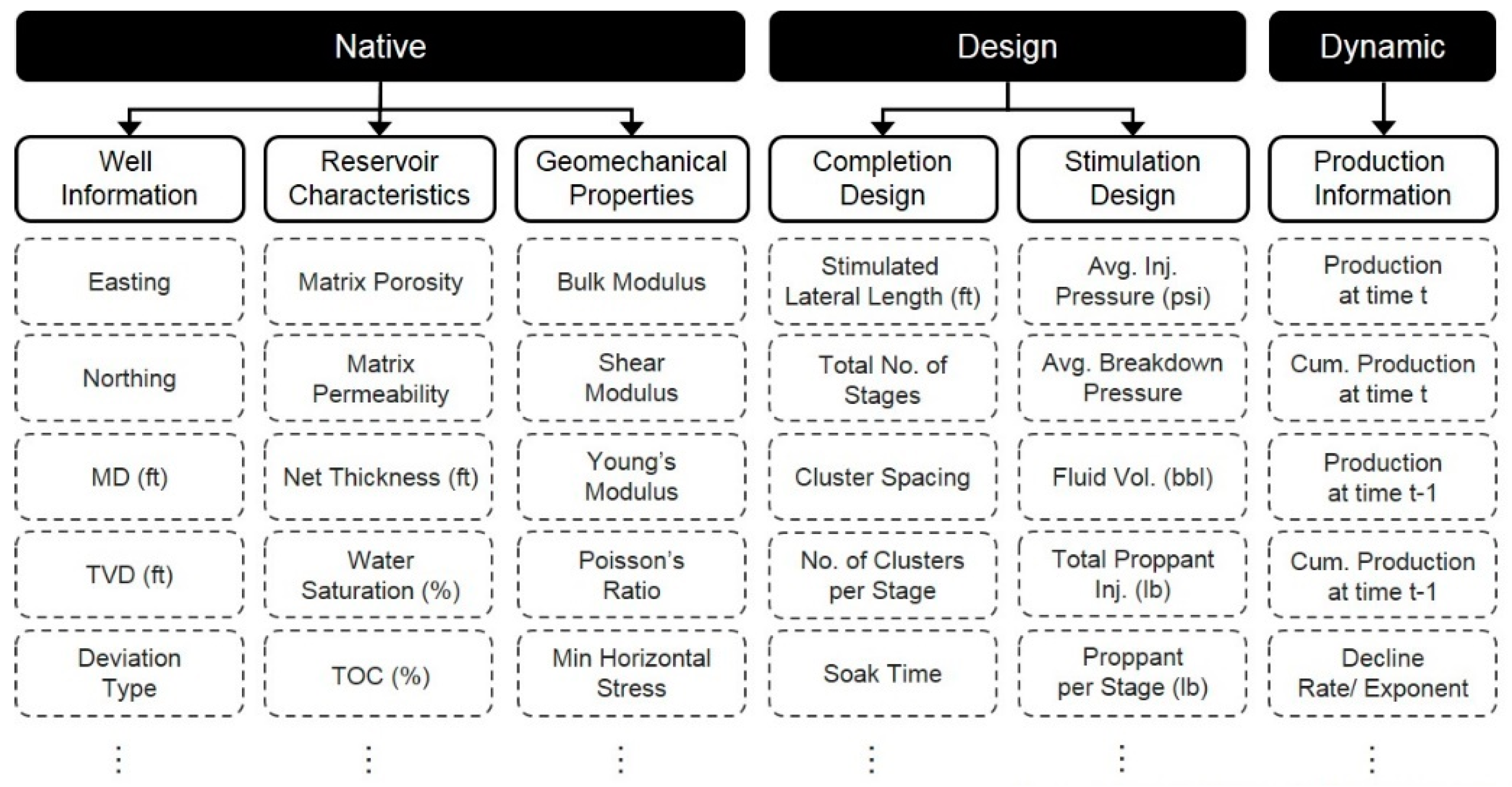
1.1. Production-Related Attributes
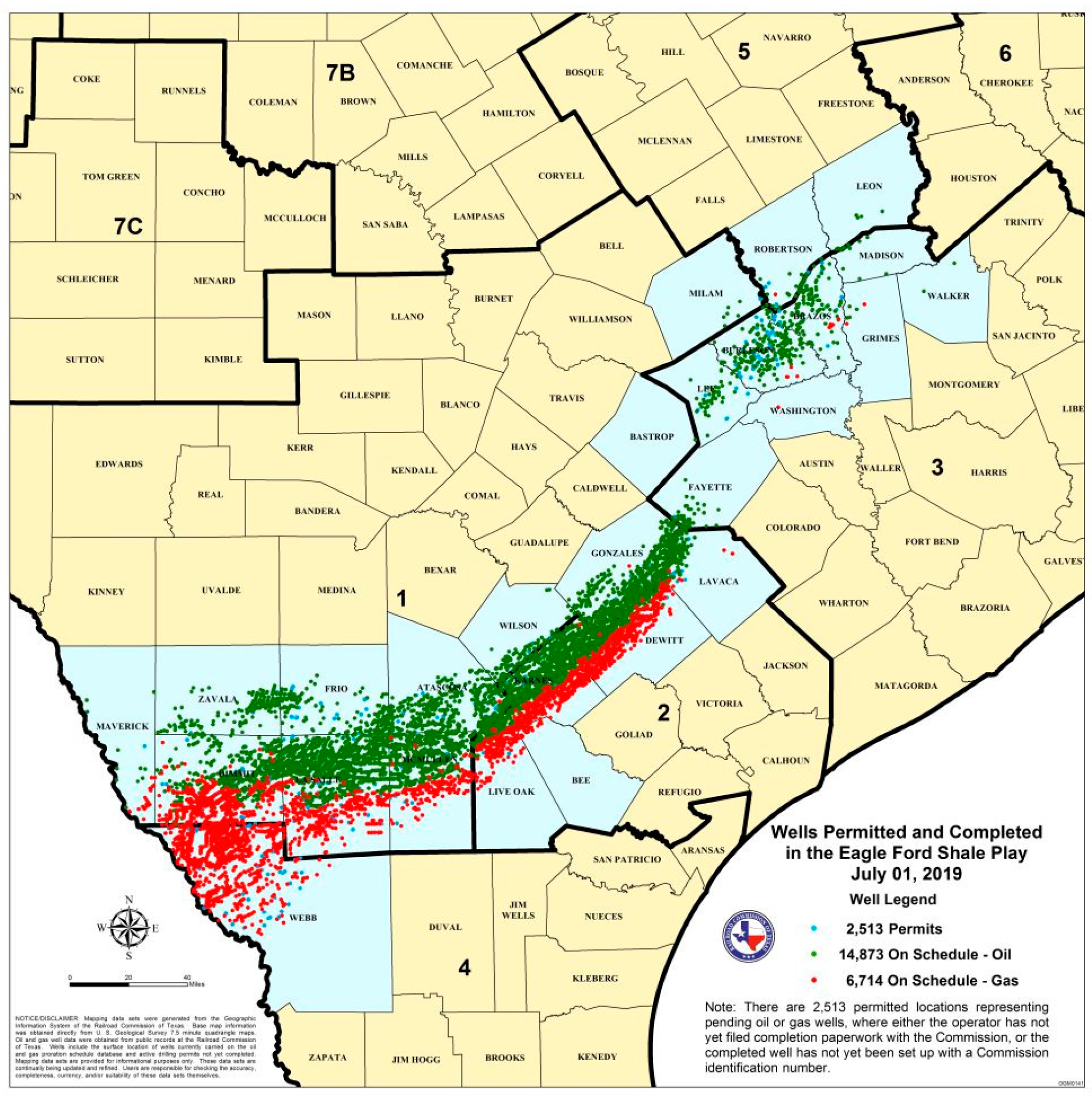
1.2. Study Area
2. Production Estimation Method in Shale Formations
2.1. Decline Curve Analysis
2.2. Probabilistic Method
2.3. Research Trends
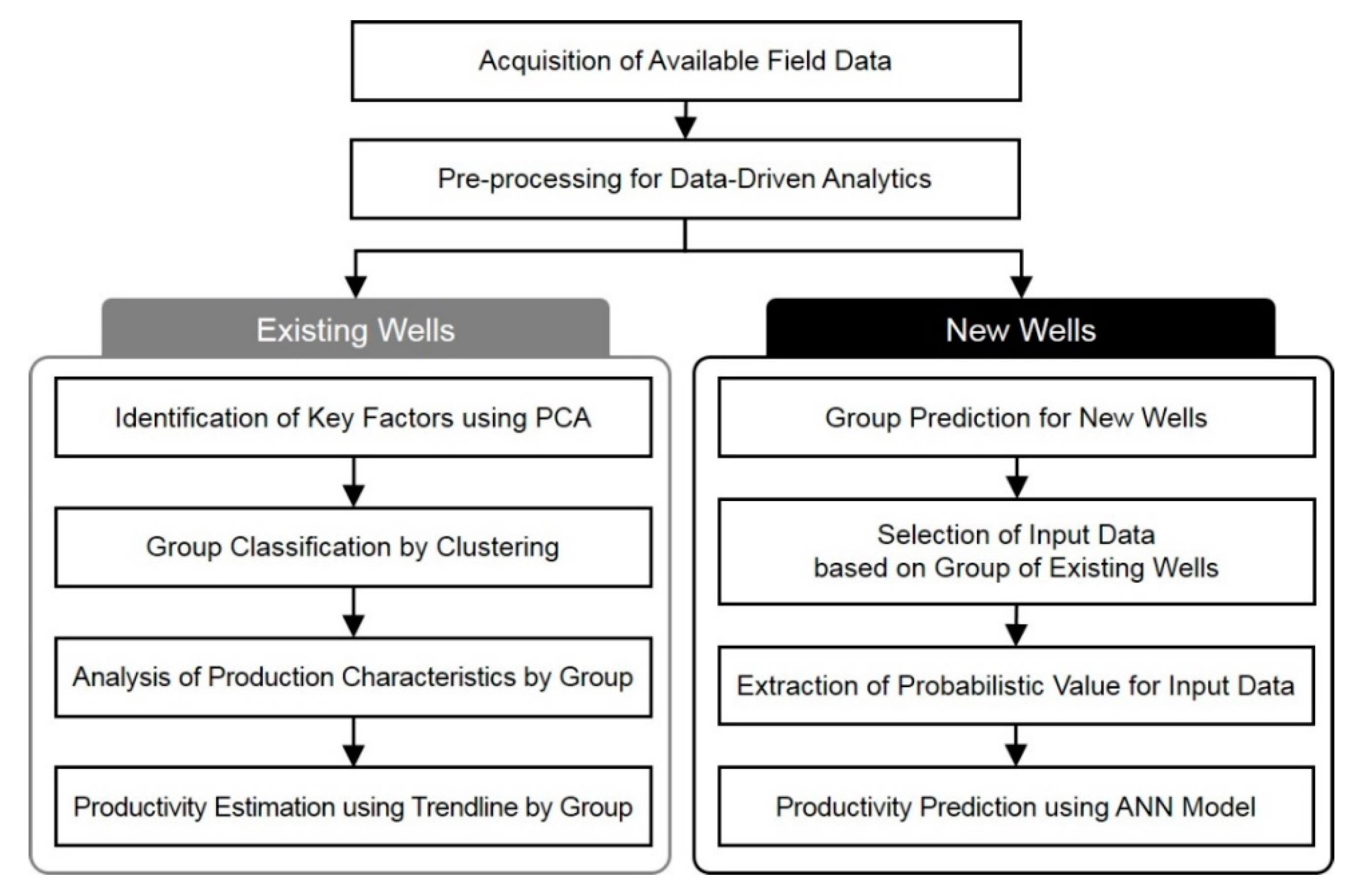
3. Data-Driven Analytics of Production Characteristics in Shale Formations
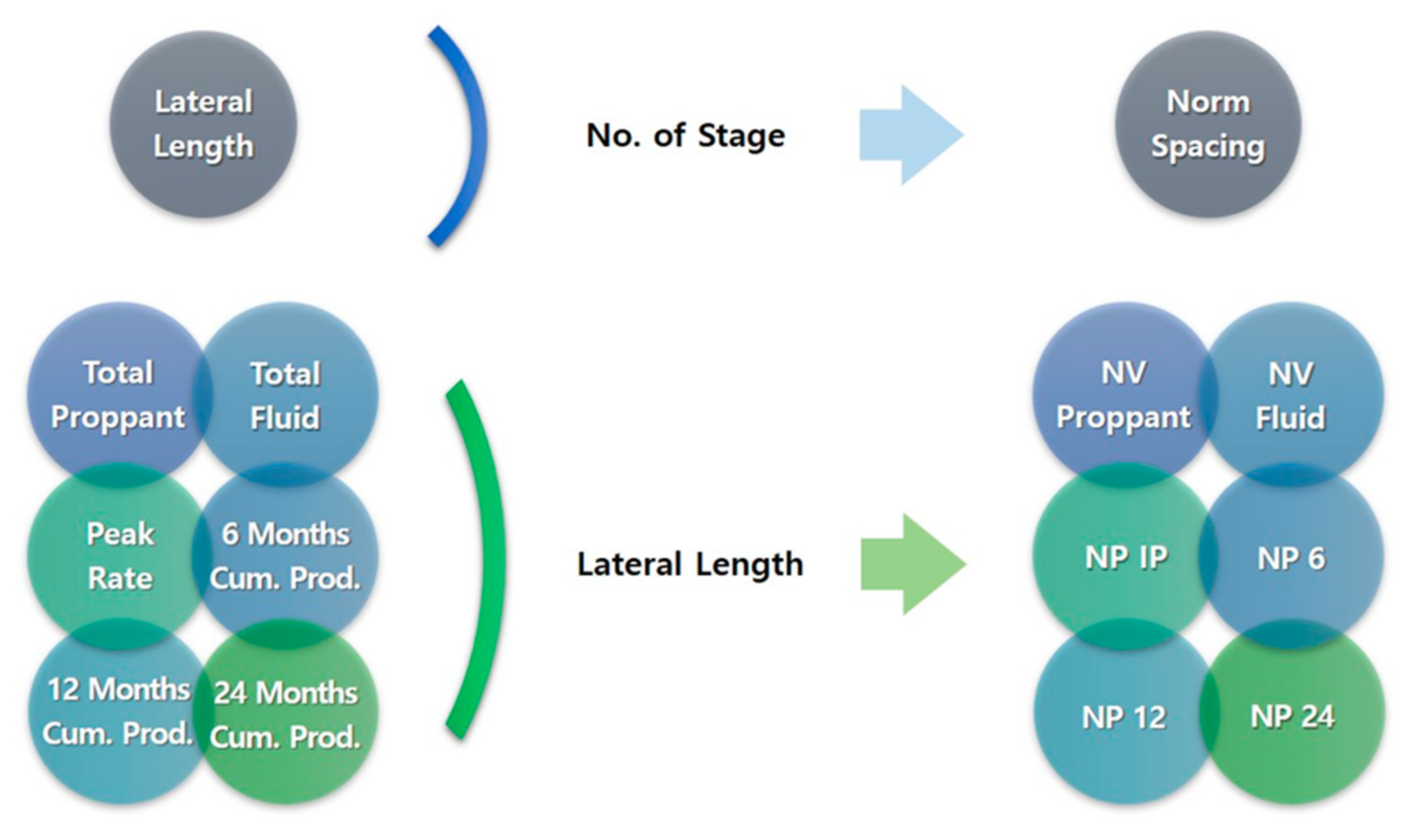
3.1. Feature Selection and Extraction for Identifying Key Factors
3.2. Unsupervised Learning for Group Classification
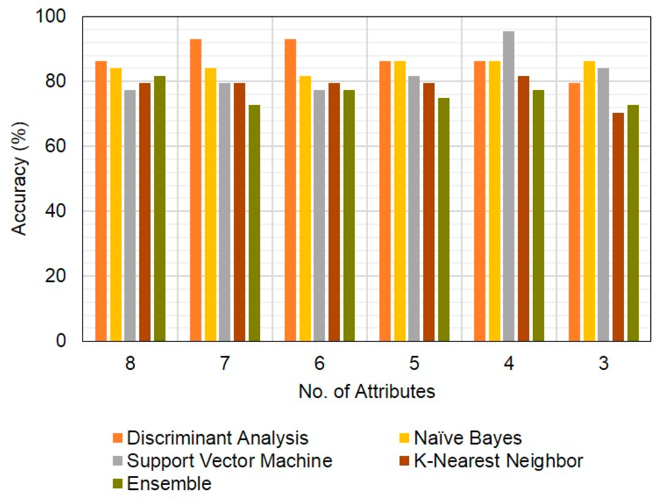
3.3. Supervised Learning for Classified Group Estimation
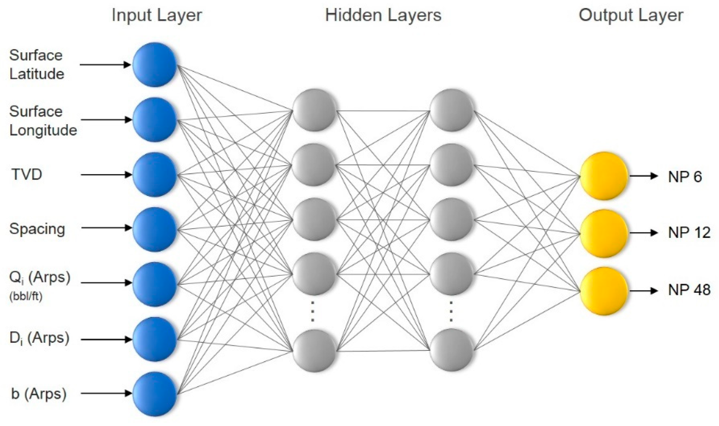
3.4. Artificial Neural Networks for Production Forecasting
4. Analysis of the Existing Wells
4.1. Acquisition of Field Data and Preprocessing
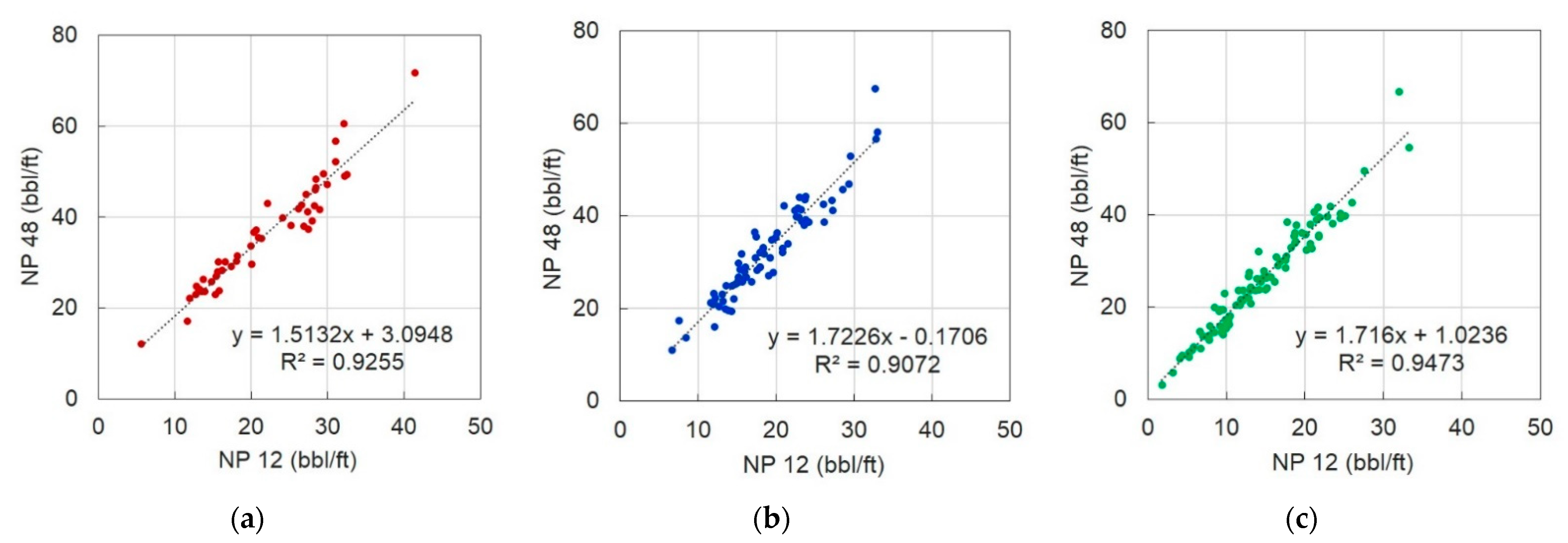
4.2. Identification of Correlations and the Key Factors
4.3. Analysis of Production Characteristics Using Group Classification
4.4. Production Estimation Using Classified Groups
5. Analysis of the New Wells
5.1. Probability Input and Feature Extraction by Group
5.2. Case Study of Input Attributes for Group Estimation
5.3. Development and Validation of ANN Model
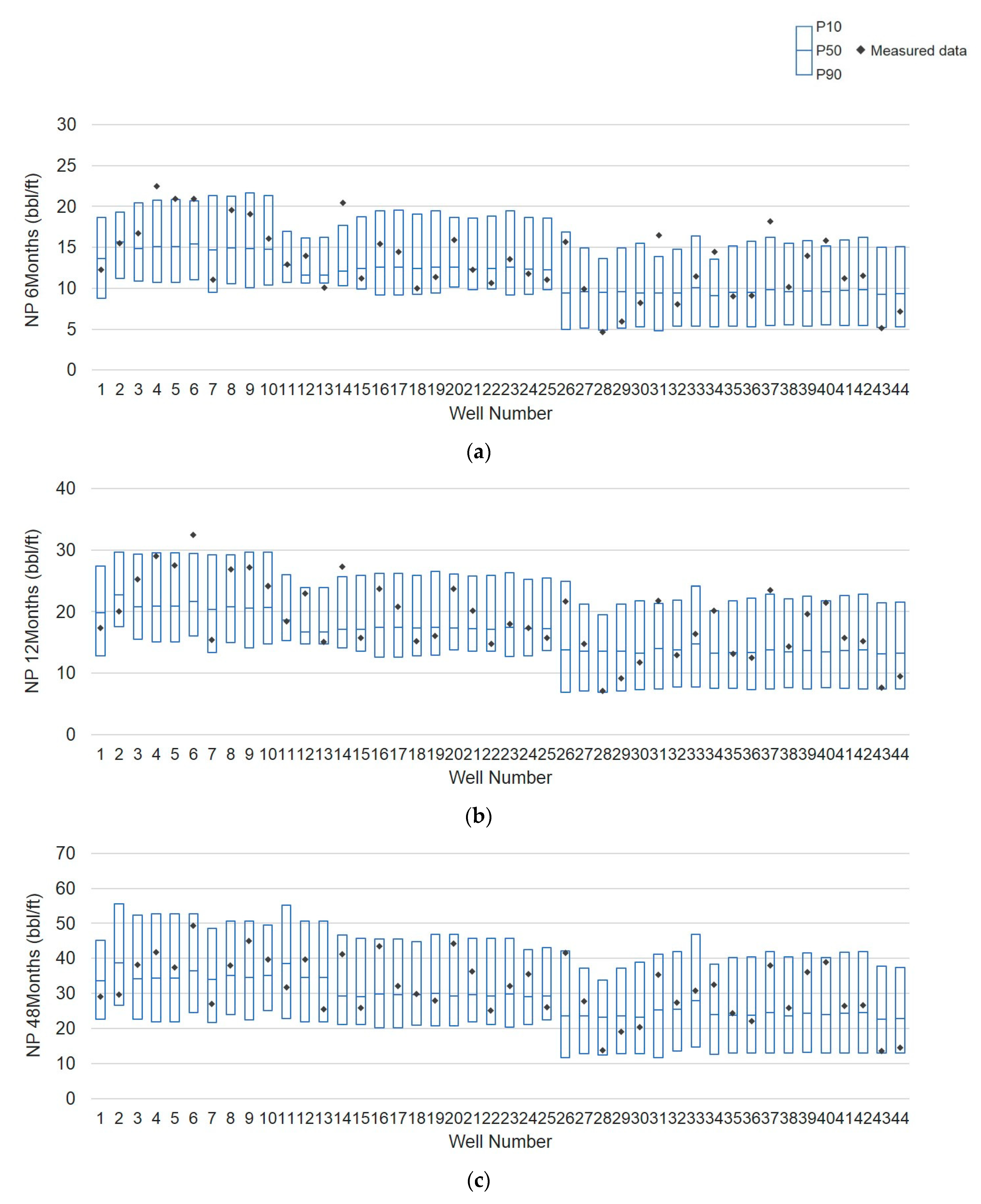
5.4. Prediction of Probabilistic Production
6. Discussion
Author Contributions
Funding
Institutional Review Board Statement
Informed Consent Statement
Conflicts of Interest
References
- U.S. Energy Information Administration (EIA). Annual Energy Outlook 2021 with Projections to 2050. Available online: https://www.eia.gov/outlooks/aeo/pdf/00%20AEO2021%20Chart%20Library.pdf (accessed on 12 March 2021).
- Cao, Q.; Banerjee, S.; Gupta, S.; Li, J.; Zhou, W.; Jeyachandra, B. Data Driven Production Forecasting using Machine Learning. In Proceedings of the SPE Argentina Exploration and Production of Unconventional Resources Symposium, Buenos Aires, Argentina, 1–3 June 2016. SPE-180984-MS. [Google Scholar]
- Suhag, A.; Ranjith, R.; Aminzadeh, F. Comparison of Shale Oil Production Forecasting using Empirical Methods and Artificial Neural Networks. In Proceedings of the SPE Annual Technical Conference and Exhibition, San Antonio, TX, USA, 9–11 October 2017. SPE-187112-MS. [Google Scholar]
- Sun, X.; Ma, X.; Kazi, M. Comparison of Decline Curve Analysis DCA with Recursive Neural Networks RNN for Production Forecast of Multi Wells. In Proceedings of the SPE Western Regional Meeting, Garden Grove, CA, USA, 22–27 April 2018. SPE-190104-MS. [Google Scholar]
- Klie, H.; Florez, H. Data-Driven Discovery of Unconventional Shale Reservoir Dynamics. In Proceedings of the SPE Reservoir Simulation Conference, Galveston, TX, USA, 10–11 April 2019. SPE-193904-MS. [Google Scholar]
- Mohaghegh, S.D. Shale Analytics: Data-Driven Analytics in Unconventional Resources, 1st ed.; Springer: Berlin, Germany, 2017; ISBN 978-3319487519. [Google Scholar]
- Gaurav, A. Horizontal Shale Well EUR Determination Integrating Geology, Machine Learning, Pattern recognition and MultiVariate Statistics Focused on the Permian Basin. In Proceedings of the SPE Liquids-Rich Basins Conference—North America, Midland, TX, USA, 13–14 September 2017. SPE-187494-MS. [Google Scholar]
- Alabboodi, M.J.; Mohaghegh, S.D. Conditioning the Estimating Ultimate Recovery of Shale Wells to Reservoir and Completion Parameters. In Proceedings of the SPE Eastern Regional Meeting, Canton, OH, USA, 13–15 September 2016. SPE-184064-MS. [Google Scholar]
- Li, Y.; Han, Y. Decline Curve Analysis for Production Forecasting Based on Machine Learning. In Proceedings of the SPE Symposium: Production Enhancement and Cost Optimisation, Kuala Lumpur, Malaysia, 7–8 November 2017. SPE-189205-MS. [Google Scholar]
- He, Q. Smart Determination of Estimated Ultimate Recovery in Shale Gas Reservoir. In Proceedings of the SPE Eastern Regional Meeting, Lexington, KY, USA, 4–6 October 2017. SPE-187514-MS. [Google Scholar]
- Vyas, A.; Gupta, A.D.; Mishra, S. Modeling Early Time Rate Decline in Unconventional Reservoirs Using Machine Learning Techniques. In Proceedings of the Abu Dhabi International Petroleum Exhibition and Conference, Abu Dhabi, United Arab Emirates, 13–16 November 2017. SPE-188231-MS. [Google Scholar]
- Bowie, B. Machine Learning Applied to Optimize Duvernay Well Performance. In Proceedings of the SPE Canada Unconventional Resources Conference, Calgary, AB, Canada, 13–14 March 2018. SPE-189823-MS. [Google Scholar]
- BuKhamseen, N.Y.; Ertekin, T. Validating Hydraulic Fracturing Properties in Reservoir Simulation Using Artificial Neural Networks. In Proceedings of the SPE Kingdom of Saudi Arabia Annual Technical Symposium and Exhibition, Dammam, Saudi Arabia, 24–27 April 2017. SPE-188093-MS. [Google Scholar]
- Tandon, S. Integrating Machine Learning in Identifying Sweet Spots in Unconventional Formations. In Proceedings of the SPE Western Regional Meeting, San Jose, CA, USA, 23–26 April 2019. SPE-195344-MS. [Google Scholar]
- Mohaghegh, S.D.; Gaskari, R.; Maysami, M. Shale Analytics: Making Production and Operational Decisions Based on Facts: A Case Study in Marcellus Shale. In Proceedings of the SPE Hydraulic Fracturing Technology Conference and Exhibition, The Woodlands, TX, USA, 24–26 January 2017. SPE-184822-MS. [Google Scholar]
- Amr, S.; El Ashhab, H.; El-Saban, M.; Schietinger, P.; Caile, C.; Kaheel, A.; Rodriguez, L. A Large-Scale Study for a Multi-Basin Machine Learning Model Predicting Horizontal Well Production. In Proceedings of the SPE Annual Technical Conference and Exhibition, Dallas, TX, USA, 24–26 September 2018. SPE-191538-MS. [Google Scholar]
- Grechka, V.; Li, Z.; Howell, B.; Garcia, H.; Wooltorton, T. Microseismic imaging of unconventional reservoirs. In Proceedings of the 2018 SEG International Exposition and Annual Meeting, Anaheim, CA, USA, 14–19 October 2018. SEG-2018-2995627. [Google Scholar]
- Hetz, G.; Kim, H.; Datta-Gupta, A.; King, M.J.; Przybysz-Jarnut, J.K.; Lopez, J.L.; Vasco, D. History Matching of Frequent Seismic Surveys Using Seismic Onset Times at the Peace River Field, Canada. In Proceedings of the SPE Annual Technical Conference and Exhibition, San Antonio, TX, USA, 9–11 October 2017. SPE-187310-MS. [Google Scholar]
- Baek, S.; Akkutlu, I.Y.; Lu, B.; Ding, S.; Xia, W. Shale Gas Well Production Optimization using Modified RTA Method—Prediction of the Life of a Well. In Proceedings of the SPE/AAPG/SEG Unconventional Resources Technology Conference, Denver, CO, USA, 22–24 July 2019. URTEC-2019-185. [Google Scholar]
- Economides, M.J.; Nolte, K.G. Reservoir Stimulation, 3rd ed.; Wiley: Hoboken, NJ, USA, 2000; ISBN 978-0471491927. [Google Scholar]
- Shin, H.D.; Lee, K.S.; Jang, I.S.; Park, C. Unconventional Resources Development; CIR: Seoul, Korea, 2015; ISBN 979-1156101765. [Google Scholar]
- Wigwe, M.E.; Bougre, E.S.; Watson, M.C.; Giussani, A. Comparative evaluation of multi-basin production performance and application of spatio-temporal models for unconventional oil and gas production prediction. J. Petrol. Explor. Prod. Technol. 2020, 10, 3091–3110. [Google Scholar] [CrossRef]
- Ma, Y.Z.; Holditch, S. Unconventional Oil and Gas Resources Handbook: Evaluation and Development, 1st ed.; Gulf Professional Publishing: Oxford, UK, 2015; ISBN 978-0128022382. [Google Scholar]
- Wigwe, M.E.; Bougre, E.S.; Watson, M.C.; Giussani, A. Spatio-temporal Models for Big Data and Applications on Unconven-tional Production Evaluation. In Proceedings of the SPE/AAPG/SEG Unconventional Resources Technology Conference, Austin, TX, USA, 20–22 July 2020. URTEC-2020-2855. [Google Scholar]
- Satter, A.; Iqbal, G.M. Reservoir Engineering: The Fundamentals, Simulation, and Management of Conventional and Unconventional Recoveries, 1st ed.; Gulf Professional Publishing: Oxford, UK, 2015; ISBN 978-0128002193. [Google Scholar]
- James, S. Shale Gas Production Processes, 1st ed.; Gulf Professional Publishing: Oxford, UK, 2013; ISBN 978-0124045712. [Google Scholar]
- Texas RRC. Eagle Ford Shale Information. Available online: www.rrc.texas.gov/oil-and-gas/major-oil-and-gas-formations/eagle-ford-shale/ (accessed on 10 August 2021).
- Arps, J.J. Analysis of Decline Curves. Trans. AIME 1945, 160, 228–247. [Google Scholar] [CrossRef]
- Seshadri, J.N.; Mattar, L. Comparison of Power Law and Modified Hyperbolic Decline Methods. In Proceedings of the Canadian Unconventional Resources and International Petroleum Conference, Calgary, Alberta, Canada, 19–21 October 2010. SPE-137320-MS. [Google Scholar]
- Clark, A.J.; Lake, L.W.; Patzek, T.W. Production Forecasting with Logistic Growth Models. In Proceedings of the SPE Annual Technical Conference and Exhibition, Denver, CO, USA, 30 October–2 November 2011. SPE-144790-MS. [Google Scholar]
- Yu, S.; Miocevic, D.J. An Improved Method to Obtain Reliable Production and EUR Prediction for Wells with Short Production History in Tight/Shale Reservoirs. In Proceedings of the SPE/AAPG/SEG Unconventional Resources Technology Conference, Denver, CO, USA, 12–14 August 2013. URTEC-1563140-MS. [Google Scholar]
- Joshi, K.; Lee, W.J. Comparison of Various Deterministic Forecasting Techniques in Shale Gas Reservoirs. In Proceedings of the SPE Hydraulic Fracturing Technology Conference, The Woodlands, TX, USA, 4–6 February 2013. SPE-163870-MS. [Google Scholar]
- Shin, H.J.; Kim, J.S.; Lim, J.S. Application of various deterministic decline curve analyses in resource plays. Geosyst. Eng. 2015, 18, 61–72. [Google Scholar] [CrossRef]
- Kang, P.S.; Shin, H.J.; Lim, J.S. Effect of Shale Reservoir Property and Condition of Hydraulic Fracture on Decline Curve Analysis Factor. J. Korean Soc. Miner. Energy Resour. Eng. 2017, 54, 223–232. [Google Scholar] [CrossRef]
- Kurtoglu, B.; Cox, S.A.; Kazemi, H. Evaluation of Long-Term Performance of Oil Wells in Elm Coulee Field. In Proceedings of the Canadian Unconventional Resources Conference, Calgary, AB, Canada, 15–17 November 2011. SPE-149273-MS. [Google Scholar]
- Meyet Me Ndong, M.P.; Dutta, R.; Burns, C. Comparison of Decline Curve Analysis Methods with Analytical Models in Unconventional Plays. In Proceedings of the SPE Annual Technical Conference and Exhibition, New Orleans, LA, USA, 30 September–2 October 2013. SPE-166365-MS. [Google Scholar]
- Rezaee, R. Fundamentals of Gas Shale Reservoirs, 1st ed.; Wiley: Hoboken, NJ, USA, 2015; ISBN 978-1118645796. [Google Scholar]
- Shin, H.J.; Lim, J.S.; Shin, S.H. Estimated ultimate recovery prediction using oil and gas production decline curve analysis and cash flow analysis for resource play. Geosyst. Eng. 2014, 17, 78–87. [Google Scholar] [CrossRef]
- Gonzalez, R.; Gong, X.; McVay, M. Probabilistic Decline Curve Analysis Reliably Quantifies Uncertainty in Shale Gas Reserves Regardless of Stage of Depletion. In Proceedings of the SPE Eastern Regional Meeting, Lexington, KY, USA, 3–5 October 2012. SPE-161300-MS. [Google Scholar]
- Kim, J.S.; Shin, H.J.; Lim, J.S. Probabilistic Decline Curve Analysis for Forecasting Estimated Ultimate Recovery in Shale Gas Play. J. Korean Soc. Miner. Energy Resour. Eng. 2014, 51, 808–819. [Google Scholar] [CrossRef]
- Shin, H.J.; Hwang, J.Y.; Lim, J.S. Probabilistic Prediction of Estimated Ultimate Recovery in Shale Reservoir using Kernel Density Function. J. Korean Inst. Gas 2017, 21, 61–69. [Google Scholar] [CrossRef]
- Luo, G.; Tian, Y.; Bychina, M.; Ehlig-Economides, C. Production Optimization Using Machine Learning in Bakken Shale. In Proceedings of the SPE/AAPG/SEG Unconventional Resources Technology Conference, Houston, TX, USA, 23–25 July 2018. URTEC-2902505-MS. [Google Scholar]
- U.S. Energy Information Administration (EIA). The Number of Drilled but Uncompleted Wells in the United States Continues to Climb. Available online: https://www.eia.gov/todayinenergy/detail.php?id=39332 (accessed on 29 April 2021).
- Perrier, S.; Delpeint, A.; Shawutii, Z.; Shrestha, A. Machine-Learning Based Analytics Applied to Stimulation Performance in the Utica Shale: Case Study and Lessons Learned. In Proceedings of the SPE/AAPG/SEG Unconventional Resources Technology Conference, Houston, TX, USA, 23–25 July 2018. URTEC-2902017-MS. [Google Scholar]
- Chen, C.; Gao, G.; Gelderblom, P.; Jimenez, E. Integration of cumulative-distribution-function mapping with principal-component analysis for the history matching of channelized reservoirs. SPE Reserv. Eval. Eng. 2016, 19, 278–293. [Google Scholar] [CrossRef]
- Lim, J.S.; Kang, J.M.; Kim, J. Multivariate Statistical Analysis for Automatic Electrofacies Determination from Well Log Measurements. In Proceedings of the SPE Asia Pacific Oil and Gas Conference, Kuala Lumpur, Malaysia, 14–16 April 1997. SPE-38028-MS. [Google Scholar]
- Yoo, H.J.; Lim, J.S.; Kim, S.J. Electrofacies determination from well logs using fuzzy clustering analysis. J. Korean Soc. Miner. Energy Resour. Eng. 2009, 46, 424–430. [Google Scholar]
- Tan, P.; Steinbach, M.; Karpatne, A.; Kumar, V. Introduction to Data Mining, 2nd ed.; Pearson: London, UK, 2018; ISBN 978-0133128901. [Google Scholar]
- Zaefferer, M. Optimization and Empirical Analysis of an Event Detection Software for Water Quality Monitoring. Master’s Thesis, Technical University of Cologne, Cologne, Germany, June 2012. [Google Scholar]
- MathWorks. Machine Learning. Available online: https://kr.mathworks.com/campaigns/offers/machine-learning-with-matlab.html (accessed on 10 August 2021).
- Politecnico di Milano. A Tutorial on Clustering Algorithms. Available online: https://matteucci.faculty.polimi.it/Clustering/tutorial_html/index.html (accessed on 11 August 2021).
- Harwood, C.; Wipat, A. Methods in Microbiology; Academic Press: Cambridge, MA, USA, 2012; Volume 39, ISBN 978-0080993874. [Google Scholar]
- Theodoridi, S.; Koutroumbas, K. Pattern Recognition, 4th ed.; Academic Press: Cambridge, MA, USA, 2008; ISBN 978-0123744913. [Google Scholar]
- Angelov, P.P.; Gu, X. Empirical Approach to Machine Learning; Springer: Berlin, Germany, 2019; ISBN 978-3030023836. [Google Scholar]
- Cunningham, P.; Delany, S.J. K-Nearest Neighbour Classifiers; Technical Report UCD-CSI-2007-4; School of Computer Science & Informatics, University College Dublin: Dublin, Ireland, 2007. [Google Scholar]
- Hastie, T.; Tibshirani, R.; Friedman, J. The Elements of Statistical Learning: Data Mining, Inference, and Prediction, 2nd ed.; Springer: Berlin, Germany, 2009; ISBN 978-0387848570. [Google Scholar]
- Ertekin, T.; Silpngarmlers, N. Optimization of formation analysis and evaluation protocols using neuro-simulation. J. Petrol. Sci. Eng. 2005, 49, 97–109. [Google Scholar] [CrossRef]


| Author(s) | [9] | [10] | [11] | [12] | [42] |
|---|---|---|---|---|---|
| Basin | Reservoir simulation | Marcellus | Eagle Ford | Duvernay | Bakken |
| Fluid | Oil & Gas | Gas | Oil | Oil | Oil & Gas |
| Well Num. | 100 | 100 | 120 | 262 | 2061 |
| Method | ANN [7 50 3] | ANN [20 20 1] | RF SVM MARS | LR Multiple LR ANN | Deep learning [8 4*100 1] |
| Input | 7 | 20 | 9 | 21 | 8 |
|
|
|
|
| |
| Output | LGM (K, a, n) | 50 years EUR | DCA parameters & EUR (Arps, SEPD. Duong, Weibull) | Well performance (individual well/type curve) | 1-year production by stage |
| Results | R 0.92 | The points of the actual and predicted data are almost identical | RMSE (for EUR) 45,32,44,30 (RF) 44,31,43,29 (SVM) - (MARS) | R2 0.41 (LR) 0.76 (multi LR) 0.93 (ANN) | R2 0.75 (training) 0.61 (testing) |
| Author(s) | [15] | [16] |
|---|---|---|
| Basin | Marcellus | DJ, Williston, Anadarko, Powder River |
| Fluid | Oil & Gas | Oil |
| Well no. | 128 | 713 (DJ) |
| Method | ANN [9 15 1] | Extreme gradient boosting tree (xgbTree) (Best performing of 7 algorithms) |
| Input | 9 | 31 |
|
| |
| Output | 6-month Cum. production | Arps (q, Di, EUR) (one of each parameter) |
| Results | R2 0.96 (training) 0.77 (testing) | Accuracy (%) (for best case) 97.31, 87.82, 93.27 (PLs) 81.89, 80.97, 76.74 (NPLs) |
| Native | Design | Dynamic |
|---|---|---|
| Surface latitude | Lateral length (ft) | NP IP (bbl/ft) |
| Surface longitude | HF stage | NP 6 months (bbl/ft) |
| Bottom hole latitude | Norm spacing (ft/stage) | NP 12 months (bbl/ft) |
| Bottom hole longitude | NVP (lbs/ft) | NP 24 months (bbl/ft) |
| Measured depth (ft) | NVF (bbl/ft) | NP (Arps) (bbl/ft) |
| True vertical depth (ft) | (Arps) | |
| Landing direction (degree) | (Arps) | |
| Choke size | ||
| County number | ||
| Well elevation (ft) |
| Case 1 | Case 2 | Case 3 | Case 4 |
|---|---|---|---|
| County num. | Surface latitude | MD | TVD |
| Surface latitude | Surface longitude | TVD | HF stage |
| Surface longitude | MD | Lateral length | Norm spacing |
| Well elevation | TVD | HF stage | NVP |
| Landing direction | Lateral length | Norm spacing | NVF |
| MD | HF stage | NVP | |
| TVD | Norm spacing | NVF | |
| Lateral length | NVP | NP 6 | |
| HF stage | NVF | ||
| Norm spacing | NP 6 | ||
| NVP | Di (Arps) | ||
| NVF | b (Arps) | ||
| NP 6 | |||
| Choke size | |||
| Di (Arps) |
| Cluster 1 | Cluster 2 | Cluster 3 | |
|---|---|---|---|
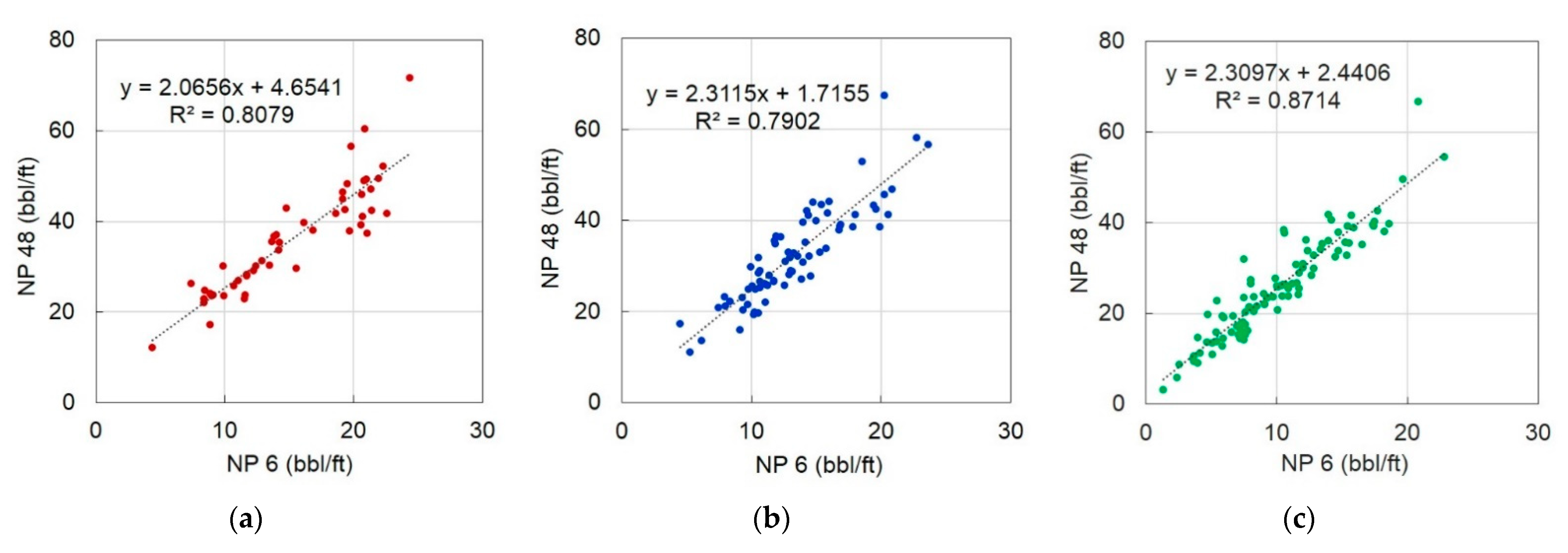
| NP 6 vs. NP 48 | 9.72% | 12.02% | 12.60% |
| NP 12 vs. NP 48 | 6.44% | 7.94% | 7.87% |
| Cluster 1 | Cluster 2 | Cluster 3 | |||||||
|---|---|---|---|---|---|---|---|---|---|
| P10 | P50 | P90 | P10 | P50 | P90 | P10 | P50 | P90 | |
| Initial production rate (bbl/ft/Month) | 1.95 | 3.25 | 4.97 | 1.99 | 2.89 | 4.57 | 1.03 | 2.18 | 3.73 |
| Initial decline rate | 0.10 | 0.20 | 0.28 | 0.15 | 0.25 | 0.32 | 0.14 | 0.23 | 0.31 |
| Decline exponent | 0.25 | 0.59 | 0.88 | 0.33 | 0.68 | 0.99 | 0.49 | 0.73 | 1.02 |
| 8 Attributes | … | 5 Attributes | … | 3 Attributes |
|---|---|---|---|---|
| TVD | TVD | Norm Spacing | ||
| Lateral Length | HF Stage | NVP | ||
| HF Stage | Norm Spacing | NVF | ||
| Norm Spacing | NVP | |||
| NVP | NVF | |||
| NVF | ||||
| NP IP | ||||
| NP 6 |
Publisher’s Note: MDPI stays neutral with regard to jurisdictional claims in published maps and institutional affiliations. |
© 2021 by the authors. Licensee MDPI, Basel, Switzerland. This article is an open access article distributed under the terms and conditions of the Creative Commons Attribution (CC BY) license (https://creativecommons.org/licenses/by/4.0/).
Share and Cite
Shin, H.-J.; Lim, J.-S.; Jang, I.-S. Probabilistic Prediction of Multi-Wells Production Based on Production Characteristics Analysis Using Key Factors in Shale Formations. Energies 2021, 14, 5226. https://doi.org/10.3390/en14175226
Shin H-J, Lim J-S, Jang I-S. Probabilistic Prediction of Multi-Wells Production Based on Production Characteristics Analysis Using Key Factors in Shale Formations. Energies. 2021; 14(17):5226. https://doi.org/10.3390/en14175226
Chicago/Turabian StyleShin, Hyo-Jin, Jong-Se Lim, and Il-Sik Jang. 2021. "Probabilistic Prediction of Multi-Wells Production Based on Production Characteristics Analysis Using Key Factors in Shale Formations" Energies 14, no. 17: 5226. https://doi.org/10.3390/en14175226
APA StyleShin, H.-J., Lim, J.-S., & Jang, I.-S. (2021). Probabilistic Prediction of Multi-Wells Production Based on Production Characteristics Analysis Using Key Factors in Shale Formations. Energies, 14(17), 5226. https://doi.org/10.3390/en14175226