1. Introduction
Within the technological development in the automotive industry, the evaluation of energy efficiency in reciprocating internal combustion engines (ICE) has always established new monitoring guidelines towards a common goal: to establish new methodologies for the reduction in the consumption of fossil fuels, being these elements non-renewable, as well as the reduction in the emission of polluting gases, greenhouse gases and particles from this thermal process [
1].
Even though the feasibility of electrified powertrains in medium-duty and heavy-duty busses and trucks, both for passengers and freight, will be ready in the near future, nowadays, the diesel engine still maintains its hegemony over the rest of configurations, mainly due to the low production costs of fuel, as well as the continuous improvements in terms of performance, fuel consumption and pollutant emissions.
Currently, the scientific community, builders and designers follow three main lines to achieve these objectives [
2]:
Establish methodologies that improve energy efficiency and the performance of existing propulsion systems.
Establish a transition towards the use of fuels with lower carbon content (natural gas, hydrogen, renewable fuels and electricity).
Develop technologies for capturing and transforming the gases resulting from the combustion process into products with a less harmful effect on nature (catalysts, NOx reduction systems, particle filters).
Following the first line of action, for the establishment of methodologies to improve the efficiency and performance on thermal machines, it is important to analyze the influence of all the elements that participate in the combustion process: the technical and technological configuration of the engine (naturally aspirated or supercharged), the qualitative characteristics of the fuel and the environmental conditions (atmospheric pressure, temperature and humidity) in which the whole phenomenon occurs.
Thus, the increase in the altitude at which the engine of a vehicle works, with the consequent reduction in pressure and atmospheric temperature, has an effect on the air composition and density, and consequently, on the performance of diesel reciprocating combustion engines, being this effect more important in naturally aspirated technologies [
3]. Within their research on the effect of environmental conditions on operation [
4], the authors establish the need to use the atmospheric hydrostatic equation, based on considering a certain temperature profile (isothermal or triangular), as a way of estimating the composition of the air, thus predicting the molar fraction of oxygen and nitrogen in the air, and thus estimating the air density at each of the points.
Based on this difference in the composition of the air, the explanation about the decrease in performance of an ICE, due to the variation in altitude, focuses, on the one hand, on the change in the ratio between the amounts of air and fuel that enter the combustion chamber (i.e., the operating fuel-air ratio) and, on the other hand, both in the variation of the volumetric efficiency, as the capability of the reciprocating engine to renew the air mass in the cylinder, as well as in the indicated performance, since, in these conditions, the pressure in the cylinder is lower throughout the entire engine cycle. This decrease in indicated performance implies that the weight of mechanical losses increases over the decreased indicated power and, therefore, the relative loss of effective power is even greater than the indicated power.
The increase in altitude notably decreases the indicated power, and therefore, the effective power, also causing an extension of the delay period to ignition, an increase in the maximum heat release rate and a reduction in the combustion duration throughout the range of engine speed [
3]. This effect is minimized in the case of supercharged engines [
5]. The decrease in oxygen in the air translates into a higher specific fuel consumption BSFC of the engine, which in vehicle terms, means an increase in fuel consumption referred to the distance traveled (L/100km).
In the case of emissions, the altitude influences on certain characteristic parameters in the diesel combustion process, such as the adiabatic temperature of the flame, the delay time and the lift-off length, both in naturally aspirated and supercharged engines, whose effect on NOx emissions, for example, represented a decrease of around 11% for altitudes of 1850 MASL (meters above sea level) in natural aspiration, and of 2% for altitudes between 1600 and 2160 MASL in supercharged configurations [
4]. According to [
6], NOx is formed in the combustion processes in such a way that its composition depends on the maximum combustion temperature and its temporal evolution, the combustion pressure and the oxygen concentration. These effects of altitude on NOx emissions depend on different variables [
7]. Due to the increase in altitude, the maximum temperature in the cylinders decreases, because the maximum pressure in the cylinder also decreases, caused by a lower pressure at the intake valve closing.
Regarding the formation of carbon monoxide (CO) and unburned hydrocarbons (HCs), the dependence on environmental factors is due to changes in temperature and pressure that have been generated in the combustion chamber. In this way, with the increase in altitude, the internal pressure of the cylinder decreases, which causes an increase in jet-to-wall impingements, as the main phenomenon of generation of the aforementioned emissions [
7]. Finally, the soot formation is well known as the result of an incomplete combustion process, generally accentuated at higher altitude, having as a main effect on this environmental condition a greater delay in self-ignition, which would cause a shorter delayed combustion phase.
Other researchers have analyzed the effect on emissions in greater detail, considering two operating conditions when the engine works at a high latitude, and the amount of air is reduced: if the amount of injected fuel is reduced in order to maintain the fuel-air ratio, or if the amount of fuel remains constant or even increases (to compensate the internal efficiency loss).
To evaluate these effects due to the variation of the environmental characteristics in the combustion process in diesel engines, methodologies based on computational mathematical models or experimental models can be followed. The computational models for the complete estimation of the performance characteristics, fuel consumption and emissions of polluting gases in ICE, such as the AVL BOOST™ software package, provide a very complete, economical and intuitive interface with quite exact results.
Other works use computational models to predict diesel engines behavior, such as those specified in [
8,
9,
10], focusing on improving engine performance taking into account environmental condition changes.
These simulation methodologies are an option to choose, especially in countries with less access to advanced measurement technology (to acquire data either in engine laboratory or in driving conditions). Experimental methodologies, even having the advantage of directly evaluating the results on the physical motor, have the disadvantage of being very expensive, taking too much time in preparation and calibration, as well as the difficulty to obtain explicit cause and effect relationships from the results.
Thus, applying computational mathematical models, an investigation conducted by [
11] analyzed a diesel system for naturally aspirated engines, with a range of analysis between 0 MASL and 4500 MASL, in different operating regimes, verifying a reduction of 5–10% in the generated power, also verifying the proportional improvement of the system (approximately 24%) with the use of turbocharged systems. On the other hand, it was estimated the behavior of a diesel engine under various conditions of temperature and ambient pressure, using both diesel and ethanol and methanol in the combustion process, showing a reduction in the in-cylinder pressure when the temperature in the intake manifold increases [
12]. These authors concluded that, in the case of ethanol, the highest combustion pressure (174.8 bar) occurs at an ambient temperature of 30 °C, while with the use of diesel as fuel, a lower pressure peak would occur (103.9 bar) at an ambient temperature of 50 °C.
Experimentally, the effect of environmental conditions on the diesel combustion process has been extensively studied. Thus, the effects of the increase in altitude in heavy-duty diesel engines were verified, both for atmospheric pressures recorded in Detroit (989 hPa) and for two simulated altitudes in Denver (826 hPa) and Mexico City (779 hPa), under constant fuel conditions controlled by DDEC II [
13]. The results showed that at full load, the torque decreases slightly with increasing altitude, while in the field of emissions of HC, CO and PM, there is a growth in these emissions where, for example, the emissions of CO increased by 60%, and that of PM by 47% when it went from 989 hPa to 779 hPa of atmospheric pressure.
Meanwhile, focusing mainly on naturally aspirated diesel engines, a 10% decrease in NOx was visualized in a 1980 Caterpillar 3208 engine increasing altitude from 1800 MASL to 3050 MASL [
14]. In parallel, it was denoted an increase in HC, CO and smoke emissions in these experimental conditions, while [
15] found a 40% increase in the emission of soot when passing from 350 MASL to 975 MASL, mainly due to the decrease in the density of the air in the intake, causing incomplete combustion in direct injection diesel engines. In addition, an experimental chamber was described for testing engines with the capability of reproducing the ambient pressure and temperature under high altitude conditions (up to 7000 MASL) [
16,
17]. The engine tests can be in stationary conditions and also simulate the dynamic behavior in a vehicle driving cycle.
Currently, the introduction of turbocharged systems has represented a substantial improvement, both in the increase in performance and the reduction in fuel consumption and emissions, but even these engines are not free from experiencing the effects of the variation of environmental conditions. Thus, for example, it was analyzed the behavior of a turbocharged diesel engine, comparing it at altitude ranges between 150 MASL and 3000 MASL [
17]. They showed that the dynamic behavior of a variable geometry turbine during the EDC driving cycle generates high pressure peaks in the exhaust manifold that, added to the low charge pressures at the intake, reduce the indicated efficiency with the consequent increase in BSFC and emissions. The performance of these systems when they experiment altitude variations are limited due to three main factors: the pressure limits in the cylinder, the average speed of the turbine and the temperature reached at the exhaust [
11], in addition to the functional design limits of the diesel engine [
18].
Another important factor to consider is the engine load and the regime, as analyzed by [
18,
19], who stated that as the altitude increases, the emission of HC, CO, NOx and smoke are increased in a diesel engine, especially at speeds of 2000 rpm when, for example, under special engine operating conditions (full load and low rpm), the reduction in HC and NOx emissions can be observed at high altitudes, or higher efficiency conditions observed at higher fuel injection temperatures and decreased ignition delay time.
On the other hand, research on the behavior of the type of fuel under these environmental conditions provides a complementary perspective to the analysis of performance, fuel consumption and emissions that is equally interesting. In this way, it was observed that in diesel engines using biodiesel and diesel with ultra-low sulfur concentration (ULSC), the pressure drop in the intake manifold has a negative impact not only on efficiency and power delivered, but also on emissions, where small differences were verified by the properties of each fuel [
20]. In the case of using methanol, ethanol and conventional diesel at 30 °C, it was observed that since methanol has a much higher vapor pressure compared to the other two fuels, the different properties of the fuel lead to different behaviors in the combustion process according to the environmental conditions in which it is carried out [
12].
Finally, another atmospheric variable to study, although its participation in the combustion phenomenon is lower, is the environmental humidity. The state of the art in this case follows different trends since, for example, researchers such as [
3] prefer not to address this effect since the humidity correction is usually incorporated in the pressure term of the equation, subtracting from this the pressure of atmosphere water vapor to calculate the amount of air present. There are investigations that describe in a more extended way the participation of humidity in the combustion process. The authors of [
21] showed results with a reduction in NOx, as well as a lower amount of PM at various levels of humidity in the air, and an increase in CO in the same conditions. It should be noted that these results always demonstrated an effect of humidity lower than those of ambient temperature and pressure, which are much more noticeable.
The individual influence of each of the environmental factors studied is presented through a series of sensitivity coefficients, based on both absolute values and relative percentages, regarding variation in atmospheric temperature (°C), pressure (bar) and relative humidity (%). In a first stage of development, the performance and fuel consumption are characterized under reference conditions, provided by the manufacturer, to subsequently visualize its behavior under the environmental conditions typical of each of the cities.
The parameterization of the individual effect of each of these factors is of great relevance by means of two levels of analysis: regional and local. In the regional analysis, the effect of altitude on engine performance is considered when atmospheric pressure decreases from 1012.8 hPa (Guayaquil, 13 MASL) to 813.2 hPa (Ambato, 2500 MASL), while the associated average temperature varies from 26.5 °C to 12.5 °C, respectively. In the local analysis, alterations of the local reference conditions at each city are considered due to the presence of anticyclone (local increase in atmospheric pressure) and storm (local reduction in atmospheric pressure), together with variations in temperature (in intervals of 20 K from 0 °C to 40 °C) and relative humidity (0% (dry air), 40%, 60% and 100%).
Furthermore, analytical expressions are obtained of the individual effect of atmospheric pressure and temperature on the performance variables and pollutant emissions. These analytical expressions are statistical correlations, in the form of power laws of pressure and temperature, built from the results provided by the simulation code when the input ambient conditions are changed. CO2 emissions are derived from the fuel consumption results. Changes in these greenhouse emissions due to the use of different fuels are accounted for by the emission factor of each fuel, including renewable ones.
In summary, this work is aimed to express in a quantitative form the influence of the environmental conditions associated with altitude changes on performance engine variables (BMEP, BSFC) and emissions (CO2, NOx, CO and Soot). The work is systematic in the approach and complete in the sense of providing sensitivity coefficients for each output variable associated with changes in pressure, temperature and air humidity conditions. These conditions respond to an extensive parametric study that covers the changes in pressure and temperature from a city at sea level to a city at 2500 MASL (regional variation). Moreover, local changes in pressure and temperature at each city are also considered to evaluate the effects of a local increase in pressure (anticyclone) and similarly, a local decrease in pressure (storm). As comprehensive results of computing all operative conditions, correlations in the form of power laws summarize the quantitative effects on each engine output variable, both performance (BMEP, BSFC) and emissions, as a first approximation of engine behavior when altitude is modified.
3. Subject and Research Methods
For the development of this work, a computational model has been used included in the AVL BOOST™ software package. The procedure requires, on the one hand, the introduction of the design values of the ADE360N Diesel engine provided by the manufacturer, and on the other hand, meteorological information registered by the National Institute of Meteorology and Hydrology of Ecuador to account for the reference atmospheric conditions at several altitudes.
3.1. ADE360N Engine Simulation Model Using AVL BOOST™
The engine considered for the analysis of the influence of environmental conditions on its operating cycle is a naturally aspirated Mercedes Benz ADE 360N Series Engine, 6 cylinders in-line and a displacement of 5.958 L.
The main technical specifications of the motor are listed in
Table 1, while the connection model, flow direction and mechanical operation in the code are presented in
Figure 2.
A naturally aspirated diesel engine has been selected, without the use of an exhaust post-treatment system, as it is representative of most of the interurban passenger transport buses in Ecuador and other Latin American countries, as well. Due to the naturally aspirated characteristics of the engine, a high dependence of performance on altitude and ambient conditions can be expected.
3.2. Orographic Configuration of the Selected Cities of Ecuador
Environmental conditions have a great impact on transport performance within countries, such as those located in Latin America. Ecuador, in addition to other countries located in the area of the Andes Mountains in South America, has a very typical characteristic that distinguishes it from other countries in the world: a clear difference in altitude, temperature and humidity at different points on its national map, with consequences for the performance, consumption and emissions of polluting gases in the reciprocating internal combustion engines used in vehicles.
Continental Ecuador, being divided into three main regions (Coast, Sierra and Amazon region), has all the characteristics to exemplify the influence of environmental conditions in various types of configurations according to the city to be analyzed. To carry out the research, five representative cities were considered: Guayaquil (4 MASL), Tena (598 MASL), Santo Domingo de los Tsáchilas (1000 MASL), Santa Isabel (1641 MASL), Baños de Agua Santa (1815 MASL) and Ambato (2500 MASL). The altitudes and reference environmental characteristics of these cities are presented in
Table 2.
Based on the real pressure and temperature profile corresponding to the environmental conditions in each of the cities, making use of the expressions in Equations (4)–(6), with a triangular profile
, the values of the relevant variables are calculated for each city for dry air (
Table 3) and humid air (
Table 4).
3.3. Model Tuning for Reproduction of the Engine Manufacturer Performance Curves
The methodology developed in this work should be considered as a first order approach to estimate engine performance when environmental conditions associated with altitude change. As a first order, we mean that the AVL BOOST™ model options have been considered to simulate the engine combustion using a double Wiebe Law to impose the Heat Release Rate. This approach has the advantage of relative simplicity and less calculation time, which has made it possible to carry out a very complete parametric study. A higher order approach would require including all the complex relationships associated with the injection process, mixture formation, combustion and pollutant generation that occur in a diesel engine. It should be noted that by varying the altitude from 4 to 2500 MASL, the ambient conditions are significantly modified, so that the lower order effects can be considered secondary.
Within the scope of engine definition, all the relevant information and dimensions are included, i.e., the engine configuration (see
Figure 2), the geometric dimensions, as well as the valve timing values associated with the gas exchange processes. From these values, the model can calculate the amount of air admitted in the engine at each operating point (pressure, temperature, humidity, operating conditions), and therefore, the changes in the amount of air per cylinder and cycle when these conditions change.
In relation to the fuel injection system, the relevant information used is the amount of fuel injected per cylinder per cycle, which is calculated from the fuel mass flow rate. The process of injection and formation of an air–fuel mixture inside the cylinder is not modeled, although there is obviously a quantity of fuel that is introduced into the cylinder and determines the total amount of Heat Release in each cycle.
Inside the combustion chamber, a two-zone model is considered so that the temperatures of the two zones are calculated: burned and unburned. Associated with these temperatures, the chemical composition of each zone is calculated to take into account the formation of combustion products and pollutant emissions. As said, the combustion process inside the combustion chamber is simulated by specifying the Rate of Heat Release (ROHR), using a Wiebe’s Law function, with two components, one for premixed combustion and one for diffusion combustion.
For the kinetic production coefficients of NOx, CO and soot, the standard values proposed in the AVL BOOST™ code have been adopted. The model implemented for NOx emissions is the one proposed by [
24], taking into account six reactions based on the well-known Zeldovich mechanism. The CO model is based on the proposed by [
25] and considers two reactions of CO with OH and O
2. Finally, considering that a two-zone calculation model is selected, then the soot model is based on [
26], taking into account two reactions, one for formation and another for oxidation, both governed by kinetic mechanisms. The soot formation is attributed to the combustion rate of the diffusion combustion. The soot oxidation reaction depends on the actual net soot mass in the cylinder and the oxygen availability in the burned zone.
The expressions presented in
Section 2 have been used to establish the input conditions related to the air density and composition when the altitude changes, in particular, the ratio between the amount of nitrogen and oxygen, as well as the effect of the relative humidity of the air.
The tuning of the AVL BOOST™ model to the engine was performed considering the engine performance curve provided by the manufacturer. Based on the detailed engine geometry, including the valve timing for intake and exhaust and the operating conditions for homologation, the calibration of the model has been performed, achieving a very good agreement between the values predicted by the model and the manufacturer’s values in terms of performance and thermofluid variables (as can be seen in
Table 5. The AVL BOOST™ model also provides the simulated emissions values, although detailed information is not available from the engine manufacturer. Since the objective is to analyze the influence to changes in environmental conditions by means of sensitivity coefficients, this approach has been considered appropriate.
To fine-tune the engine simulation model, a first step to cover is reproducing its performance curves for the conditions set by the manufacturer (0 MASL, 1013.25 hPa, 20 °C and 50% relative humidity). Based on this preliminary objective, a process diagram is established within the simulation in AVL BOOST™, considering three stages: first environmental conditions, ADE360N engine geometrical parameters and fuel properties (heating value, stoichiometric fuel-air ratio
); second operating fuel-air ratio
F; and third the combustion processes and combustion law (
Figure 3).
From these input data (columns in right part of
Table 5), torque, power and BSFC curves are obtained for different engine rpm, as well as the emissions of
and other pollutants. Additionally, the values of air and fuel mass flow rates (kg/s) are included, since they are derived results that can be obtained by using the Equations (27) and (29) of following paragraphs.
As can be seen in
Figure 4, the simulation model provides very similar results with respect to engine manufacturer data, maintaining an approximation error between −3.33% and 0.67% for results in torque simulation. Since these errors are below 5%, the model can be considered tuned to reproduce the engine performance in the reference conditions, as a previous step before its use for the estimation and parameterization of the effect of environmental conditions.
To determine the coherence of the results obtained, a series of characteristic engine efficiencies [
27] have been calculated and plotted in
Figure 5, such as volumetric efficiency (
), effective efficiency (
), indicated efficiency (
) and mechanical efficiency (
), for each of the rpms studied and considering both dry and humid air (marked with an asterisk). For different calculations, an average equivalence ratio
(lean mixture,
) has been considered. The calculated values are within the expected ranges and have correct trends when varying the engine speed.
3.4. Estimation of Input Values to the AVL BOOST™ Model for Different Altitudes
Following the validation of the simulation model, regarding the results under experimental conditions proposed by the manufacturer, it is necessary to establish a methodology to set the input data for the conditions of each of the cities to be studied, as a starting point for the estimations of the brake mean effective pressure BMEP, volumetric efficiency , the absolute fuel-air ratio , the air mass flow rate and the fuel mass flow rate .
As pointed out by [
3], in order to relate the engine indicated power at some altitude conditions with the corresponding value at reference conditions, an analytical expression involving the ratios of atmospheric pressure and temperature at altitude z and their associated reference values can be used:
Additionally, it is assumed that the same functional dependence of the indicated power can also be applied for the effective power. This consideration is based on two main premises: first, that the indicated power decreases with altitude mainly because the pressure in the cylinder is lower throughout the entire cycle of the engine, and second, that the mechanical losses also experiment a slight reduction with altitude, due to lower in-cylinder pressure. This last reason justifies that many authors assume that the mechanical loss is a constant fraction of the indicated power, which means that the ratio of effective powers is equivalent to the ratio of indicated powers.
Based on this assumption, and considering that in a given engine, for each rpm, the mean effective pressure is proportional to the effective power, then Equation (24) can be expressed as follows:
In the scientific literature, the values of the exponents a and b depend on the characteristics of the engine and operating conditions. Thus, specifically for engines such as the ADE 360N Series, the exponent
a is usually equal to
in naturally aspirated diesel engines [
3]; for the exponent
b, the ISO 3046-1 standard suggests the value of
, while other authors recommend using the value
, which is the one used in this work.
It is also necessary to estimate the volumetric efficiency
in each atmospheric condition. By considering a definition of volumetric efficiency associated with the geometry and the air density calculated with conditions (pressure, temperature) at the intake manifold [
27], the only effect on the volumetric efficiency that is considered is that of the ambient temperature when it changes with altitude, in the form of power dependence as expressed in Equation (26), with an exponent
:
Once the modified values of both the effective mean pressure and the volumetric efficiency have been estimated, then the values of air and fuel mass flow rates can be determined. The air mass flow rate is given by Equation (27).
It should be noted that the pressure reduction due to altitude is transferred to the air mass flow rate only through to the change in air density, while the volumetric efficiency is pressure-independent (it only varies slightly with temperature).
The absolute fuel-air ratio can be obtained from Equation (28).
From the previous expressions, it is possible to determine the fuel mass flow rate for each altitude as:
Additionally, as detailed in the following section, when varying the altitude, it is necessary to decide whether what remains constant is the fuel-air ratio (with an associated reduction in fuel mass flow rate) or the fuel flow (with then an increase in fuel-air ratio, due to air flow reduction). The second possibility will try to keep engine effective power, although with a slight associated reduction in the effective efficiency.
3.5. Environmental Conditions and Input Data for Each City
Following the validation of the simulation model, it is necessary to establish the reference conditions of temperature, atmospheric pressure and environmental humidity for each city. From these conditions, the input data for the engine model can be estimated in order to be able to compute the engine performance at each city (providing the results for the regional analysis).
The expressions of the previous paragraph for the effect of environmental variables on engine performance have been used to estimate BEMP Equation (24) and volumetric efficiency Equation (25) and are included in
Table 6.
In parallel with these, the value of the air mass flow rate is computed by means of Equation (26), while the fuel mass flow rate is computed by Equation (28) (
Table 7).
Later, from these input data, a parametric study will be carried out by varying each atmospheric variable in certain ranges over the city reference value (providing the results of the local analysis). The process diagram is indicated in
Figure 6.
The main use of computing these flow rates (as intermediate estimations) is obtaining the values of the fuel-air ratio, used as input data in AVL BOOST™ simulations. Additionally, the fuel mass flow rate will be later used in the parametric study under the assumption of keeping it constant when the environmental conditions change. As a first approach to the simulation of the engine performance, the double Wiebe curves that establish the ROHR for each engine speed have been maintained, although a change in the shape of these curves could be expected due to second-order changes caused by modifications in the combustion delay time.
4. Results
Once the ADE360N engine model is tuned and validated, and the reference conditions at each city are established, parametric studies of the effects of independent variations in temperature, atmospheric pressure and air humidity can be performed (
Figure 7).
As can be seen in
Figure 7, both in the parametric study of temperature variation and in the atmospheric pressure variation, two levels of analysis are considered. First, a regional characteristic study is developed, by which engine performance under reference conditions is estimated for the atmospheric conditions of each city. In this considered interval, the atmospheric pressure drops from 1012.8 hPa (Guayaquil) to 813.2 hPa (Ambato), while the average temperature drops from 26.5 °C to 12.5 °C, respectively. Subsequently, on these reference values, a second level of the parametric study is established, locally, within which the pressure conditions are modified considering situations of anticyclone (local increase in pressure) and storm (local reduction in pressure), independently of temperature variation (in 20k intervals from 0° to 40 °C), as well as relative humidity (in specific intervals of 0% (dry air), 40%, 60% and 100%).
The entire set of results obtained is used in the last section to establish correlations of performance and pollutant emissions with respect to ambient pressure, temperature and humidity.
4.1. Effect of the Variation of Ambient Temperature at Each Altitude
In this first section of the parametric study of influence, a range of variation of ambient temperature is fixed between 0 °C and 40 °C (historical maximum registered in the Meteorological Yearbook of Ecuador), with intermediate values every 5 °C, for three characteristic engine speeds: 1200 rpm (low speed), 1600 rpm (medium speed) and 2400 rpm (high speed). At each city, its particular reference pressure associated to its altitude (
Table 2) is used in this set of simulations.
Although this is a temperature range acceptable for simulation, it should be emphasized that in many of the highest altitude places in Ecuador, temperatures higher than 30 °C are rarely reached, while in those closer to sea level, temperatures are almost never lower than 10 °C. Therefore, the simulated cases cover extreme values, whose experimental observation would require climatic chambers.
4.1.1. Effect on Brake Mean Affective Pressure BMEP
The analysis of BMEP is started for each city, always considering a constant fuel mass flow rate. The results in general show a BMEP decrease as the temperature locally increases, with a bigger effect in cities at higher altitude (and lower reference pressure).
Figure 8 shows the absolute values of BMEP as they are reduced due to increase in ambient temperature (0 °C–40 °C), with very similar trends for the pressure conditions corresponding to three cities (4, 1641, 2500 MASL) and three engine rpms.
It is very important to indicate that these trends can be unified for all computed conditions (pressure, rpm) as a single relative reduction in a percentage basis, as is shown in
Figure 9, with a sensitivity factor of BMEP with temperature of −0.17%/°C (or strictly speaking %/K).
4.1.2. Effect on Specific Fuel Consumption BSFC
In contrast to the decrease in BMEP with the temperature increase, specific fuel consumption BSFC increases uniformly with ambient temperature, as can be seen in
Figure 10.
As before, a sensitivity coefficient can be computed to see the relative increase in BSFC, shown in
Figure 11. Although the mean value of this coefficient is about +0.09%/°C, there are slight differences between low rpm (higher coefficient) and high rpm (smaller coefficients). In addition, the effect is also slightly more important at higher altitudes than at sea level.
4.1.3. Effect on NOx Emission
Figure 12 shows the effect of temperature on the absolute values of NOx emissions for the conditions considered. As expected, the higher the values of temperature for each reference pressure, the higher the NOx emissions.
There are, however, differences depending on the engine rpm, as can be seen in more detail in
Figure 13. The sensitivity coefficients can be estimated as 0.86%/°C at high speed (2400 rpm) (
Figure 13, box C), 0.54%/°C at medium speed (1600 rpm) and 0.47%/°C at low speed (1200 rpm) (
Figure 13, box D).
4.1.4. Effect on CO Emissions
In terms of the dependence of the estimated CO emissions on the variation in temperature,
Figure 14 shows the results for the two extreme pressures considered (4 and 2500 MASL). In general, absolute values increase with air temperature, with small differences among the engine rpms.
These differences can be seen in more detail in
Figure 15, where the sensitivity coefficient is plotted for each condition. The values range from 0.20%/°C (2400 rpm) to 0.35%/°C (1200 rpm), and the higher the altitude (lower pressure), the higher the sensitivity coefficient.
4.1.5. Effect on Soot Emissions
Figure 16 plots the results of the absolute values of soot emissions when ambient temperature increases, at the three reference pressures and three engine rpms, showing a general uniform trend.
This can also be appreciated in
Figure 17 where the relative dependence of soot emissions on temperature shows only small variations among the results relative to different pressures and engine rpms. Quantitative values of the sensitivity coefficient range between 1.51%/°C at low speed (
Figure 17, box G) and 1.81%/°C at high speed (
Figure 17, box H).
4.2. Effect of the Variation of Ambient Pressure at Each Altitude
In the case of variation of the ambient pressure, it is essential, as with the temperature, to analyze its influence both at a local level and at a comparative regional level between each of the cities, as specified at the beginning of this section.
According to this, in a first approach at a regional level, atmospheric pressure values of each of the selected cities are estimated for three determined temperature values (0 °C, 20 °C and 40 °C), at different engine speed (1200 rpm, 1600 rpm and 2400 rpm). Later, locally, a single value of ambient temperature was considered ( = 20 °C), while an increase or decrease of ± 2 kPa is introduced on the average ambient pressure of each city, to represent the increase and decrease in pressure associated with an anticyclone and a storm, respectively.
4.2.1. Effect on the Brake Mean Effective Pressure BMEP
The regional level analysis shows a decrease in performance while comparing the values obtained between Guayaquil (1.0128
) and Ambato (0.8132
), with sensitivity coefficients of 0.073 bar/kPa at low regimes (1200 rpm), 0.071 bar/kPa at medium speeds (1600 rpm) and 0.068 bar/kPa at high speeds (2400 rpm) (
Figure 18).
Locally, at a temperature of
= 20 °C, a slight difference between the presence of anticyclone (+2
) and storm (−2
) over the average BMEP value was obtained (
Figure 19), with percentage differences of ±1.13%/kPa for the city of Guayaquil (1.0128
), ±1.24%/kPa for Santa Isabel (0.9332
) and ±1.45%/kPa for Ambato (0.8132
).
4.2.2. Effect on Specific Fuel Consumption BSFC
Contrary to the decrease in performance, in the case of fuel consumption, there is an increase in both analysis levels considered in the parametric study. As seen in
Figure 20, regionally, the sensitivity coefficient of BSFC is higher at high temperatures (40 °C) with 3.41% in the whole range from 4 MASL to 2500 MASL, while at low temperatures (0 °C), it is 3.26% in the same range.
Furthermore, due to the effect of this environmental parameter, considering low operating regimes (1200 rpm), the accumulated BSFC increase is 3.27%; at medium regime (1600 rpm), it is slightly reduced to 3.21%; and finally, at high speed (2400 rpm), an increase of 3.52% holds (
Figure 20, box I).
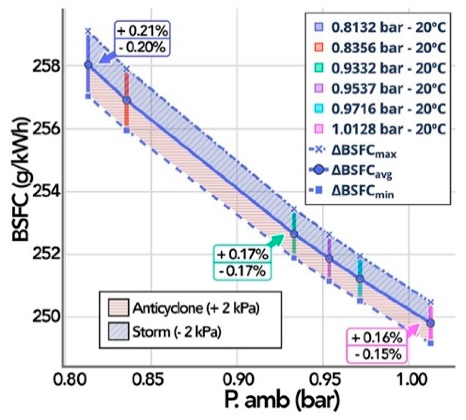
Locally, with the presence of an anticyclone (+2
), the BSFC decreased on average by −0.17%/kPa, while in storm (−2
) consumption increases by +0.18%/kPa (
Figure 21).
4.2.3. Effect on NOx Emission
Considering the atmospheric pressure difference (
), between 0 °C and 40 °C, for low operating regimes (1200 rpm), the cumulative percentage difference in the average NOx emissions is −1.00%; at medium speed (1600 rpm), it is slightly reduced to −0.65%; and finally, at high speed (2400 rpm), there is a variation of −0.56% (
Figure 22, box G).
At a local level, an increase in NOx generation is observed at low speed (1200 rpm), regarding a higher operating point (2400 rpm), with 19.51% in Guayaquil (1.0128
) and 22.78% in Ambato (0.8132
) in stormy environments (−2
), compared to 18.74% in Guayaquil (1.0128
) and 22.08% in Ambato (0.8132
) in anticyclone (+2
) (
Figure 23).
4.2.4. Effect on CO Emissions
Regionally, the trends do not follow a clear pattern, as can be seen in
Figure 24. It mainly stands out that in case of engine speed analysis, CO production would be much higher at elevated operating regimes (2400 rpm), with an average difference of 9.34 g/kWh in the whole pressure range, comparing it to low and medium speeds (1200 and 1600 rpm).
In a local analysis, in terms of anticyclone (+2
) and storm (−2
) (
Figure 25), a greater influence on CO emissions in cities with higher altitudes is shown. In this case, the CO sensitivity coefficient increases at storm with
/kPa, while in anticyclone decreases by
/kPa, unlike the city of Guayaquil (1.0128
), where the values are reduced to
/kPa and
/kPa, for storm and anticyclone, respectively.
4.2.5. Effect on Soot Emissions
Finally, from a regional point of view, unlike what happened with NOx, in the case of soot, there is a greater emission in medium and high operating regimes (1600 rpm:
= 0.93 g/kWh,
= 1.03 g/kWh) and a lower formation in low operating regimes (1200 rpm:
= 0.75 g/kWh,
= 0.82 g/kWh). As a percentage, in the case shown in
Figure 26, box O, the mentioned phenomenon is clearly observed for Ambato (0.8132
) with a variation of DSoot = 0.75% at 2400 rpm, DSoot = 0.74% at 1600 rpm and DSoot = 0.61% at 1200 rpm.
The presence of anticyclone (+2 kPa) and storm (−2 kPa) has an influence on the emission of soot higher than NOx and CO rates at local levels, with a sensitivity coefficient of
/kPa in cities with higher altitude, such as the city of Ambato (0.8132
), as observed in
Figure 27.
4.3. Effect of the Variation of Relative Humidity for Each Altitude
To illustrate the influence of air relative humidity on engine performance, fuel consumption and pollutant emissions, the results relative to the two cities with the extreme conditions will be presented: Guayaquil (4 MASL, 1.0128 ) and Ambato (2500 MASL, 0.8132 ). The effects of four relative humidity values (0% (dry air), 40%, 60% and 100% relative humidity) are studied, all of them applied at three levels of ambient temperature (0 °C, 20 °C and 40 °C).
As a first step in this parametric study, the values of all the variables that participate in the determination of the influence of ambient humidity (
Table 8 and
Table 9) are calculated: saturation pressure
in Equation (13), absolute humidity
in Equation (11) and molar pseudo fraction of water vapor
in Equation (16). In addition, according to those stated in
Section 2.2, the density of humid air of Equation (19) is also calculated, obtained by applying the correction factor
of Equation (18).
It should be noted that the AVL BOOST™ model cannot be applied directly considering humid air due to the limitations of the software for estimating pollutant emissions under these conditions. An alternative methodology to estimate emissions is to consider the influence of humidity only on the reduction in air density, without considering other aspects such as the reduction in the temperature in the combustion chamber, or characteristic changes in the behavior of the flame front, among others.
To obtain the fuel-air ratio values, initially the calculated volumetric efficiency value is kept constant, according to Equation (25), since the density changes due to the application of the correction factor , to later estimate the approximate value of the brake mean effective pressure BMEP in each of the cases Equation (24).
The resulting values of volumetric efficiency
and brake mean effective pressure BMEP are shown in
Table 10 and
Table 11, for Guayaquil and Ambato, respectively.
Once the values of volumetric efficiency , humid air density , reference effective efficiency and the theoretical estimate of BMEP have been obtained, the fuel-air ratio corresponding to each of the proposed cases can be computed, based on the application of Equation (27), always considering constant fuel mass flow rate. Once the fuel-air ratio for each operating point is fixed, all input data for the AVL BOOST™ model are completed and the code is run to generate the results of performance and emissions, as described in the following.
4.3.1. Effect of Air Relative Humidity on BMEP
The effect of the relative humidity on the BMEP is less than the effects of the variation in the temperature and the ambient pressure. The results of the BMEP calculated for the two cities considered, considering the effect of going from 0% to 100% relative humidity, can be seen in
Figure 28 in absolute values (left) and in relative values referring to 0% relative humidity. In general, there is a slight decrease in BMEP, which is more noticeable at higher temperatures (40 °C) than at medium (20 °C) and low temperatures (0 °C). Although it is true that, as can be seen in
Figure 28 (right), the reduction in BMEP can reach values of −2.5%, the environmental characteristics on which these values are obtained (T = 40 °C,
= 100%, 2500 MASL) represent extreme hypothetical cases.
4.3.2. Effect of Air Relative Humidity on Specific Fuel Consumption BSFC
As can be seen in
Figure 29, both in absolute (left) and relative (right) values, the variation of BSFC due to the influence of relative humidity is practically negligible, since the percentage values in any case range between ±0.05%.
4.3.3. Effect of Air Relative Humidity on NOx Emissions
As indicated above, for the analysis of pollutant formation (NOx, CO and soot), the influence of the air relative humidity is considered in this study through a reduction in dry air density, not including the variation of the temperature in the combustion chamber or other factors that would directly participate in its production.
As a result of this assumption, the effect of increasing the relative humidity causes a slight reduction in NOx emissions (
Figure 30). In the case of cities near sea level, such as Guayaquil (1.0128
, continuous lines), the variation is small for all ambient temperatures, the difference greater being at higher temperatures (
, T = 40 °C,
).
The effect is slightly more important as altitude increases (lower atmospheric pressure), as observed in Ambato (0.8132 , dotted lines), being more noticeable as the temperature is higher. Although at low temperatures (0 °C), the effect is practically negligible, in the case of medium temperatures (20 °C), when the relative humidity goes from 0% to 100%, a decrease is obtained. At high temperatures (40 °C), with the same increase in relative humidity, the decrease is approximately doubled ().
4.3.4. Effect of Air Relative Humidity on CO Emissions
The results of the influence of relative humidity on CO emissions show an increase within all temperature ranges, both for Guayaquil (1.0128
) and for Ambato (0.8132
), being the values of
for the first and
for the second, respectively (
Figure 31). This increase is greater (in modulus) than the reduction in the NOx emissions.
4.3.5. Effect of Air Relative Humidity on Soot Emissions
The biggest influence of air relative humidity occurs on soot emissions, with reductions in the full range 0–100% of relative humidity between
for Guayaquil (1.0128
, continuous lines) and
in Ambato (0.8132
, dotted lines) (
Figure 32). In the case of Guayaquil, at 0 °C, there is, however, a slight increase in emissions.
4.4. Statistical Correlations of Combined Effects of Temperature and Pressure
Although it is true that the individual analysis of the influence of each of the environmental factors involved in the combustion process has relevant importance, it is convenient to obtain statistical correlations to establish an analytical relationship between ambient conditions and the engine outputs: performance (BMEP), fuel consumption (BSFC) and emissions (NOx, CO and soot). To obtain the desired correlations, the process diagram shown in
Figure 33 is followed.
These statistical correlations are obtained for the specific type of engine and the environmental conditions in which its operation is established. However, the use of reference values makes possible to nondimensionalize the input data (ambient pressure and temperature) and the output variables (BMEP, BSFC, CO2, NOx, CO, soot) to obtain relationships that can be used in other similar engines.
4.4.1. Sensitivity Coefficient of BMEP
In a previous section, it has been established that the difference in BMEP due to the influence of local temperature in each city (i.e., for a fixed altitude or atmospheric pressure) is small. However, the variation of BMEP is much wider when the change in city altitude is considered at the regional level, with different atmospheric pressures.
The global effect of the variation in ambient pressure and temperature on BMEP can be represented, for each engine speed, as a surface that relates three variables (
Figure 34): BMEP (bar), temperature (°C) and pressure (bar).
One way to quantitatively characterize the sensitivity of the dependence of BMEP with respect to air temperature is considering a coefficient that represents the slope of the BEMP surface along a line of constant atmospheric pressure. The values of this coefficient, in bar/°C (strictly speaking, in bar/K), are shown in
Table 12. Since the results for each atmospheric pressure (or each city or altitude) are slightly different, the last row in the table includes the averaged values in each city.
Table 13 shows the analogous values of a coefficient of dependence of the BMEP relative to the atmospheric pressure as the slope of the BMEP surface along a constant air temperature line, expressed in bar/kPa (i.e., BMEP change in bar for 1 kPa change in atmospheric pressure). The results are presented for low temperatures (0 °C), medium temperatures (20 °C) and high temperatures (40 °C) in each of the specified engine regimes (1200 rpm, 1600 rpm and 2400 rpm). Finally, the averaged value of the coefficient of dependence of BMEP with ambient pressure for a given temperature is indicated in the last row. In this case, the coefficient indicates that the sensitivity of BMEP to atmospheric pressure is higher at lower temperatures.
These dependence coefficients of BMEP with respect to ambient temperature and pressure allow us to obtain the BMEP values at certain ambient conditions once the values in other reference conditions are known, by using a linear expression. As an example, since the BEMP at Guayaquil (1.0128 ) is 7.10 bar at 1200 rpm, considering a temperature of 20 °C, the BMEP at Ambato (0.8132 , a reduction of 20 kPa) would be 7.10 − 0.071*20 = 5.71 bar. Similarly, at Santa Isabel (0.9332 , a reduction of 8 kPa), the linear dependence predicts a value of BMEP of 6.55 bar.
A more convenient alternative to express the dependency of BMEP on the environmental variables is considering a statistical correlation, that provides a straightforward analytical function. This can be obtained by using a statistical multiple correlation tool, applied to all the results calculated by means of the simulation model, considering all the engine regimes, for all changes in pressure and ambient temperature. The results have been fitted to an expression of BMEP as power functions of temperature and pressure. All variables are nondimensionalized by using the corresponding reference values of BMEP and ambient temperature and pressure, as indicated in Equation (30).
The exponents obtained for the dependence with temperature and pressure are approximately −0.5 and 1.0, but this is a consequence of the working conditions of the simulated engine which have been adjusted to get BMEP values given by the expression Equation (24). This topic is seen in more detail at the end of this section. It should be emphasized again that, as specified in
Figure 8 and
Figure 9, the difference between the value obtained by means of the AVL BOOST™ model and the value estimated by Equation (30), in most cases, does not exceed 3%.
4.4.2. Sensitivity Coefficient of BSFC
In the same way as with the variation of BMEP, a dependence of BSFC can be obtained considering the pressure and temperature conditions dependent on the altitude in each city, which, graphically, is a three-dimensional surface for each engine regime, as seen in
Figure 35.
The values of the coefficients of the slope of BSFC surface function of ambient temperature (g/kWh/°C) along a constant pressure line at three representative cities can be seen in
Table 14, with slightly different values for each engine regime. Similarly,
Table 15 contains the corresponding coefficients of dependence of BSFC of ambient pressure (g/kWh/kPa) at constant temperature.
As for BMEP, a statistical correlation has been obtained for BSFC in the form of a power function, as seen in Equation (31), recalling that a constant fuel mass flow rate has been assumed when the air mass flow rate is changed by the pressure and temperature. The general trend, according to the results obtained by various authors, is that BSFC increases if the ambient temperature increases or the atmospheric pressure decreases.
4.4.3. Sensitivity Coefficient of CO2
Considering the specific fuel consumption BSFC given by Equation (31) and the fuel emission factor, the CO
2 emissions at reference conditions (of both fuel composition and altitude) can be expressed as:
In case a different fuel is used, with an emission factor
, and altitude z changes, the CO
2 emissions can be estimated accounting by both fuel and environmental conditions:
4.4.4. Sensitivity Coefficient for Other Emissions
To illustrate the general trends of the specific emissions of NOx, CO and soot as the environmental conditions associated with altitude change, the surfaces for a medium engine speed are shown in
Figure 36.
As general trends, it can be observed that the increase in temperature has a great influence on the specific emissions of the three pollutants considered. The effect of pressure is less important in the range of altitudes considered. Furthermore, the effect of a decrease in pressure with increasing altitude leads to a reduction in NOx emissions, while CO and soot emissions increase slightly.
The results obtained follow the same trends of the values presented in previous investigations carried out by [
19,
28,
29] on the formation of NOx and CO, and the registered data obtained by [
15,
30] on soot emissions regarding the variation of environmental conditions at different altitudes.
The values of the coefficients representing the slope of the surface of each pollutant emission are presented in
Table 16, for the temperature dependence at constant pressure, and in
Table 17, for the pressure dependence at constant temperature.
In general, except for some cases in CO emissions, both dependence coefficients show uniform trends with engine rpm, what allows obtaining averaged values, included in the last row of each table.
Following the same statistical procedure of linear regression used to obtain correlations of the combined effect of temperature and atmospheric pressure, using all the values obtained for the different engine regimes (1200 rpm, 1600 rpm and 2400 rpm), the following expressions have been obtained:
4.4.5. Goodness of Statistical Correlations
As seen before, a series of statistical correlations have been obtained that allow obtaining estimates of engine performance, fuel consumption and emissions, at altitude z, through its values of temperature and atmospheric pressure (, ), from known values of performance, fuel consumption or pollutant emission is available (, , , , ) at reference ambient conditions (, ). Each correlation is defined by specific exponents (a, b).
In order to evaluate the goodness of these statistical correlations, it is necessary to check the values of the adjusted coefficient of determination
and typical error obtained in each case (
Table 18).
Since no other published values have been found for the other engine output variables, the discussion must be based on the goodness of the correlation. A value of the adjusted coefficient of determination
close to one means the effectiveness of the independent variables to explain the values of the dependent variable. High values of
are usually associated with small values of the typical error. Looking at the values included in
Table 18, it can be said that the adjustment is very good for BMEP, BSFC and soot, and reasonably good for NOx and CO.
5. Discussion
The main objective of the work is to establish the dependence of the engine output variables with respect to environmental conditions, given by pressure, temperature and humidity. To do this, first, a general expression for the combustion reaction of fuel and air with changing composition due to altitude has been written. From this expression, the stoichiometric fuel air ratio can be expressed as the product of three terms, one depending on fuel composition (in general independent of altitude), a second one depending on air composition (dependent on altitude) and a third one depending on air specific humidity.
A methodology was developed which allows us to simulate the behavior of a naturally aspirated diesel engine of six liters of displacement and 100 kW of power, representative of engines used for public transport vehicles in Ecuador and other countries in the area. For this, an AVL BOOST™ simulation model was used, which has been tuned to reproduce the curves provided by the manufacturer at standard reference conditions. The model was then extended to predict the engine performance and emissions for operating conditions associated to different altitudes. For the sake of concretion, five cities in Ecuador, ranging from sea level to 2500 MASL, were considered, with the associated values of atmospheric pressure, temperature and air humidity.
By using the engine simulation model, the effect of each of the environmental variables was considered separately: pressure, temperature and relative humidity. These variables depend on a regional basis through altitude, which sets the values of pressure and temperature, and also the ratio between relative and specific air humidity. These environmental variables can also depend locally on meteorological conditions, through an increase or decrease in temperature or an increase or decrease in pressure due to an anticyclone or storm. In general, there is a greater influence of the variation of atmospheric pressure, compared to temperature and relative humidity, the latter environment parameter having minimal influence on the calculation results.
The quantitative effects of the environmental variables on the engine output variables (BMEP, BSFC, pollutant emissions) have been evaluated by means of sensitivity coefficients of several types. The first type is just the percentage change of a given engine output variable with respect to a reference condition when the environmental variable changes. For example, it has been shown that due to the variation of the ambient temperature between 0 °C and 40 °C, the computed values for BSFC, NOx, CO and soot have a slight growth of between 0.1%/°C and 1.6%/°C, and only the BMEP experiment has a decrease of 0.2%/°C, approximately.
In relation to atmospheric pressure, in the regional analysis, with broad atmospheric pressure variation ranges (between 1.0128 bar 13 MASL, and 0.8132 bar 2500 MASL), when atmospheric pressure reduces, there is an increase in the BSFC values (+0.17%/kPa), CO (+0.06%/kPa) and soot (+0.56%/kPa), while the BMEP and NOx experience the opposite effect: −0.98%/kPa for BMEP and −0.20%/kPa for NOx emissions. At a local level, it is assumed that an anticyclone increases atmospheric pressure +2 kPa, which leads to a slight reduction in BSFC (−0.17%/kPa), accompanied by growths in BMEP (+1.27%/kPa) and NOx emissions (+0.33%/kPa). On the other hand, a storm represents a reduction of −2 kPa, which translates to an increase in BSFC, whose percentage variation is the same as in the reduction by anticyclone. On the other hand, the emissions of CO and soot also increase in stormy conditions, where the latter pollutant emission is the one that experiences the greatest variation (+0.42%/kPa).
As for the relative humidity, its influence has been introduced in the engine model input data as a reduction in the density of dry air, resulting in practically negligible effects on the output variables (lower than 0.1%/.
A second type of sensitivity coefficient is related to evaluate the change in the absolute value of each engine performance and emission outputs as and , which are the local slopes of the surface of each output variable (BMEP, BSFC, specific emissions) when pressure (or temperature) changes at constant temperature (or pressure). The values of these dependence coefficients are slightly different depending on the environmental pressure and temperature.
Finally, the third type of dependence relationships developed are statistical correlations, in the form of power laws, which allow estimating the performance values (BMEP), specific fuel consumption (BSFC) and emissions (CO2, NOx, CO and soot), taking into account the variation in pressure and ambient temperature associated with altitude, based on a reference value for each variable. These correlations, given by Equation (30) to Equation (36), provide values very close to the values used to obtain them (the results of the AVL BOOST™ model applied to the engine), in accordance with very high adjusted coefficients of determination , as well as typical errors lower than 0.75%. Due to the limitations of the emissions sub-model, these correlations do not internally consider the effect of air humidity, but are applicable in dry air conditions, allowing the extrapolation of engine performance and emissions at reference conditions to other environmental conditions.


