Abstract
The thermal conductivity of soils is a fundamental parameter for the design of ground-source heat pump systems (GSHPs) and energy geostructures. This paper presents a comprehensive evaluation of the physical, mineralogical, and thermal characteristics of typical coastal soils from Tabasco, Mexico. Twenty-five soil samples from four different strata were studied using the thermal needle probe method, X-ray diffractometry, scanning electron microscopy, and standard geotechnical soil classification tests. The results showed a significant correlation between the dry density and porosity with the thermal conductivity of the studied samples, which ranged between 1.17 and 2.32 W m−1 K−1. The performed statistical analyses indicated that coarse-grained soils had larger thermal conductivities and higher variability than fine-grained soils. Additionally, the performance of six models to estimate the thermal conductivity of soils was validated against the experimental data. All models provided accurate estimations for fine-grained soils, but only the effective medium theory (EMT) showed an adequate fit for coarse-grained soils. The results represent one of the first datasets for the thermal properties of Mexican soils. They will contribute to the implementation of GSHPs and energy geostructures in the country and locations with similar subsoil conditions, especially where time and resources are not available for their experimental determination.
1. Introduction
The energy consumption of residential and commercial buildings in Mexico has grown at an annual average rate of 3% during the last decade [1]. Among the fastest-growing activities of this sector are space conditioning systems, which account for approximately 21% of the total electricity use [2]. This increasing demand has a significant impact on the environment, and it is an obstacle for the accomplishment of the Mexican government’s commitment to reduce its greenhouse gas emissions by 22% by 2030 [3]. In recent years, ground-source heat pump systems (GSHPs) and energy geostructures have been proposed as a viable alternative to fulfill space conditioning requirements while satisfying new energy efficiency standards for buildings [4]. The efficiency of these systems depends on the storage capacity and heat transfer characteristics of the ground; thus, an accurate characterization of local soil thermal properties is crucial for their design [5]. However, the information about the thermal properties of Mexican soils is scarce [6,7], which hinders the development of this technology in the country.
In general, conduction is the predominant mechanism for heat transfer within the ground, particularly for saturated soils. Heat conduction is a process whereby internal thermal energy is transferred from one region of the medium to another by molecular interactions [8]. In an isotropic and homogeneous soil, the heat conduction equation is
where T is the temperature (K), t is the time (s), ρ is the total density of the material (kg m−3), cs is the specific heat capacity (J kg−1 K−1), and λ is the thermal conductivity (W m−1 K−1).
The characterization of the thermal conduction parameters of soils (cs and λ) can be undertaken by in situ or laboratory tests. In situ tests evaluate larger volumes of soils under real field conditions but are costly and time-consuming. Laboratory tests are relatively inexpensive, quick, and allow for the control of boundary conditions [9]. However, several separate determinations are required to obtain a representative value of the bulk thermal properties due to inherent soil heterogeneity [5]. The most widely used in situ method is the thermal response test (TRT) [10], whereas typical laboratory tests include the thermal cell [11], the needle probe [12], and the transient plane heat source [13]. In practice, TRTs are preferred to laboratory tests since they provide additional information required for the effective design of GSHPs and energy geostructures (i.e., undisturbed ground temperature and ground heat exchanger thermal resistance, in addition to the ground thermal conductivity) [14]. Different studies suggest that thermal conductivities measured with the TRT are generally higher than those obtained by laboratory tests [15,16,17,18,19,20]. Because TRTs consider large-scale soil characteristics, they are assumed to be more representative and realistic tests. Low et al. [15] and Vieira et al. [16] compared several of these methods and concluded that the thermal needle probe is a suitable procedure to determine the thermal properties of soils for GSHPs and energy geostructure applications.
Despite their importance, in small projects, soil thermal properties are normally assumed based on recommended values for geological materials or estimated using predictive models [21]. While it is possible to satisfactorily calculate cs by adding the heat capacities of the different soil constituents according to their volume fraction [22], an accurate estimation of the thermal conductivity is complicated. The thermal conductivity of soils is influenced by various physical parameters, such as mineralogy, density, particle size and shape, water content, and temperature [8,22,23]. Accordingly, several theoretical and empirical predictive models have been proposed in the literature to estimate this parameter, providing contrasting results. The above illustrates the complexity of accurately estimating the thermal conductivity of multi-phased materials and shows the importance of evaluating the applicability of each model under local conditions.
This paper describes a systematic soil survey for the characterization of the thermal conductivity and physical and mineralogical properties of typical coastal soils from Tabasco, Mexico. Overall, twenty-five undisturbed samples from four strata were analyzed in the laboratory using the thermal needle probe method. Based on the experimental data, the relationship between several index properties and thermal conductivity was examined. Additionally, X-ray diffraction (XRD) analysis and scanning electron microscope (SEM) observations were employed to study mineralogical and microstructure characteristics of the samples, respectively. These results were used to evaluate the performance of six models for the estimation of thermal conductivity of different types of soils.
The main objectives of this study are as follows: (a) to characterize the thermal, physical, and mineralogical properties of typical coastal soils from Mexico; (b) to statistically analyze the relationship between its thermal conductivity and several index properties (e.g., water content, density, porosity); and (c) to identify the most appropriate predictive thermal conductivity model for the study site. The novel information about the thermal properties of Mexican soils will contribute to the development and design of GSHPs and energy geostructures in Mexico, but also in other places and countries with similar ground conditions, particularly when time, resources, appropriate equipment, and knowledge about this technology are not available for their experimental determination, neither in situ nor in laboratory.
2. Materials and Methods
2.1. Site Description
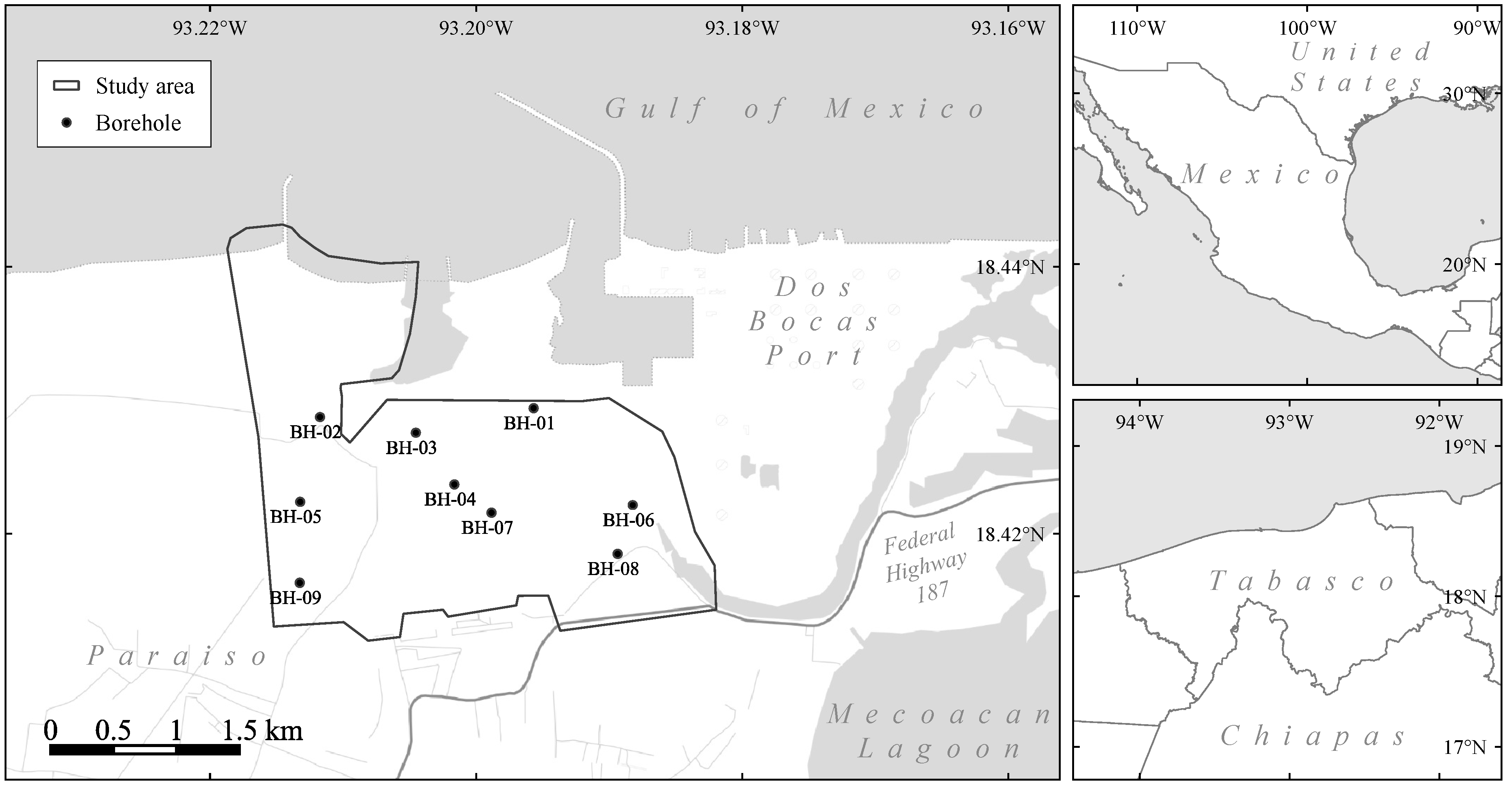
The study site is located in the municipality of Paraiso, state of Tabasco, Mexico (Figure 1). The area of approximately 13.3 km2 concentrates a wide range of commercial, industrial, and oil-related activities. It lies within the physiographic province known as the Gulf Coastal Plain and is underlain by alluvial and eolian deposits [24], producing an erratic stratigraphy in both vertical and horizontal directions. According to Zaragoza-Cardiel [25], the site stratigraphy consists of four strata. The top stratum (UG1) is a grayish-brown sand with an average thickness of 10 m. Below this, it is a gray high-plasticity clay (UG2) with shell fragments, soft consistency, and variable thickness. The third stratum (UG3) extends up to a depth of 33 m and consists of a yellowish-brown highly dense silty sand. The last stratum (UG4) is formed by an olive-gray stiff to hard lean clay with sand. The water table in the area varies between 1.5 and 5.0 m depth.

Figure 1.
Study site and borehole locations.
2.2. Material Characterization
Twenty-five samples were collected at depths varying between 4.9 and 57.5 m below the ground surface from 9 boreholes (Figure 1). The samples were obtained by smoothly pushing a stainless steel thin-wall tube (Shelby tube, 101.6 mm of outside diameter and 8.4% of area ratio) into the soil. The location and depth of the samples were selected to properly map the distribution of soil strata and provide descriptive summaries of their thermal conductivity. The collected samples were classified based on ASTM Standards [26]. Disturbed samples were used to determine water content (w), specific gravity (Gs), organic matter content (OM), particle size distribution, and Atterberg’s limits (liquid limit LL and plastic limit PL). Cubic specimens were trimmed from Shelby tubes to measure total density (ρ), dry density (ρd), porosity (n), and saturation (S) under undisturbed conditions.
Additionally, four samples representative of each soil stratum (named S07, S08, S11, S20) were selected to study their microstructural and mineralogical characteristics. The mineralogical composition was obtained by X-ray diffraction (XRD) analysis using an EMPYREAN diffractometer (PANalytical, Almelo, The Netherlands) equipped with a fine focus Cu tube (CuKα radiation), nickel filter, and PIXCel 3D detector (PANalytical, Almelo, The Netherlands) operating at 40 mA and 45 kV. For bulk powder analyses, the samples were grounded and homogenized using a pestle and agate mortar to <75 µm. Measurements were taken over a 2θ angular range from 5 to 75° with a step scan of 0.003° and an integration time of 40 s per step. To properly identify the clay minerals, clay fractions (<2 µm) were examined using XRD in air-dried form, saturated with ethylene glycol, and after heating (550 °C). XRD patterns were analyzed with the HighScore version 4.5 program (PANalytical, Almelo, The Netherlands) using reference patterns from the International Center for Diffraction Data (ICDD) and the Inorganic Crystal Structure Database (ICSD). The microstructure of the sediments was observed using a high-resolution scanning electron microscope (JEOL JSM6360LV, Jeol, Tokyo, Japan). Images at different resolutions were taken from 1-cm3 specimens previously dried by the critical point method and coated with a gold layer.
2.3. Thermal Properties Measurements
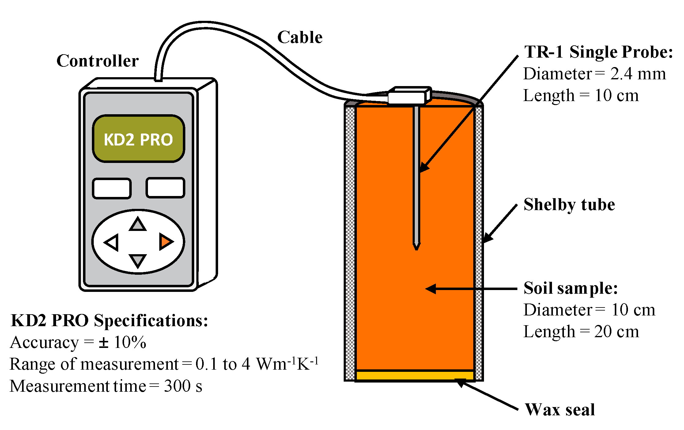
The instrument used to measure the thermal conductivity of the soil samples was the commercial manufactured thermal needle probe KD2 Pro (Decagon Devices Inc., Pullman, USA). In this study, the authors chose the TR-1 single probe (2.4 cm in diameter and 10 cm in length) because of its compliance with the specification of IEEE [27] and ASTM [12] standards. The probe measuring range is 0.1 to 4.0 W m−1 K−1 with an accuracy of ±10% (Figure 2). Its operation principle is based on the infinite line source theory of Carslaw and Jaeger [28]. The equipment monitors temperature changes caused by heat dissipation from the needle probe during a heating–recovery cycle of 300 s. The final two-thirds of the heating and recovery data are then fitted to a simplified analytical solution for heat transfer in solids that considers possible effects of temperature drift. Prior to testing, the needle probe was calibrated using glycerol and water stabilized with 5 g agar per liter.

Figure 2.
Measurement of thermal conductivity and experimental apparatus.
Three measurements were taken for each sample with a time interval of 15 min. For each sample, an adequate input power was selected to prevent any potential errors from moisture migration and evaporation. The tests were performed in undisturbed cylindrical specimens of approximately 200 mm in length and 100 mm in diameter. To minimize the amount of soil disturbance (especially in the sandy soils) and to expedite the measuring process, it is suggested the tests are carried out before extruding the samples. Thus, in this study the tube seals were carefully removed, soil surfaces were cleaned, and then the TR-1 single probe was placed to carry out the test. In soils with a soft consistency, the sensor was inserted by simply pushing it into the specimen, whereas in coarse-grained materials a 2.5 cm hole was predrilled. The probe was coated within a thin layer of thermal grease to minimize contact resistance and was allowed to achieve thermal equilibrium in the soil mass (approximately 15 min) before the first measurement.
2.4. Evaluation of Thermal Conductivity Models and Goodness-of-Fit Metrics
An accurate estimation of the thermal conductivity of soils is a complex procedure because it depends on several properties, such as mineralogy, particle size and shape, porosity, packing geometry, degree of saturation, and water content [29]. Accordingly, numerous predictive thermal conductivity models have been proposed in the literature to facilitate and improve the estimation of this property. These models are useful when the experimental measurements of the thermal conductivity are not feasible; however, their applicability must be assessed under local conditions. Farouki [8] conducted a comprehensive review of various empirical methods and found that Johansen’s model [30] gave the best prediction over a range of soil types and saturation values. More recently, Barry-Macaulay et al. [31] and Dai et al. [32] compared Johansen’s model to three of its derivative models and concluded that Cotê–Konrad [33] and Balland–Arp [34] models yielded accurate estimations. Other studies [23,29] indicate that the effective medium theory (EMT) [35], the Donazzi et al. [36], and the Gori–Corasaniti [37] models provide good agreement with experimental data, especially for soils with high degrees of saturation. In this article, the performance of the six previously mentioned models (Table 1) was validated against the experimental measurements of Tabasco coastal soils.

Table 1.
Evaluated thermal conductivity models for different types of soils a.
The evaluation of the selected models was carried out using the index properties and mineralogical compositions analysis described in Section 2.2. The values of the thermal conductivity of water (λw) and air (λa) were 0.561 and 0.025 W m−1 K−1, respectively, whereas the thermal conductivities of the soil-forming minerals were obtained from Horai [38] and Brigaud and Vasseur [39].
Goodness-of-fit between the predicted and measured values was assessed graphically via scatter plots and numerically through two statistics: (1) the coefficient of determination (R2),
and (2) the root mean square error (RMSE)
where λmod,i is the predicted thermal conductivity, λmea,i is the measured value,
is the mean of the predicted thermal conductivities, is the mean of the measure thermal conductivity, and N is the number of data. The coefficient of determination (R2) varies between 0 and 1 and measures the proportion of variance of the measured values explained by the model. RMSE is an estimator of the standard deviation of the residuals (difference between the predicted values and the measured data); the smaller the RMSE value, the better the estimation.
3. Results and Discussion
3.1. Physical, Mineralogical, and Geotechnical Characterization of the Material
Table 2 summarizes the index properties of each stratum of the study site. According to the Unified Soil Classification System (USCS) [26], the samples from UG1 and UG3 strata were classified as poorly graded sand with silt (SP-SM) or silty sand (SM), and those from UG2 and UG4 as lean clays (CL) or fat clays (CH). Most of the samples were completely saturated, except for some of the UG1 strata collected above the water table. In general, Tabasco coastal soils showed high total densities (varying between 1650 and 2290 kg/m3) and low organic matter content (less than 5%). Clayey soils exhibited low variability in most of their index properties, with coefficients of variation (CV) lower than 15%, which indicates that UG2 and UG4 strata are relatively homogeneous.
Table 2.
Descriptive statistics of index properties of the soil samples a.
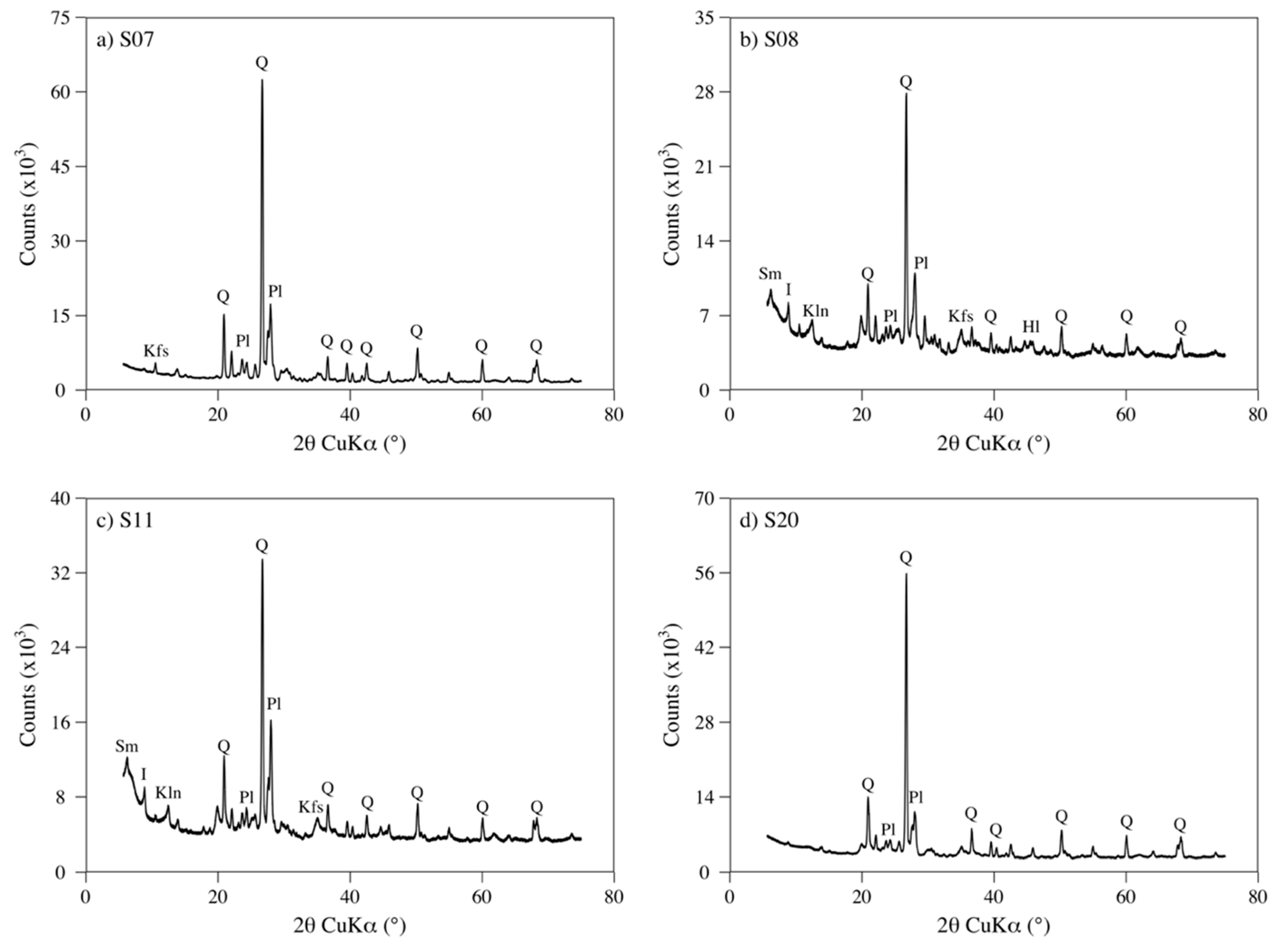
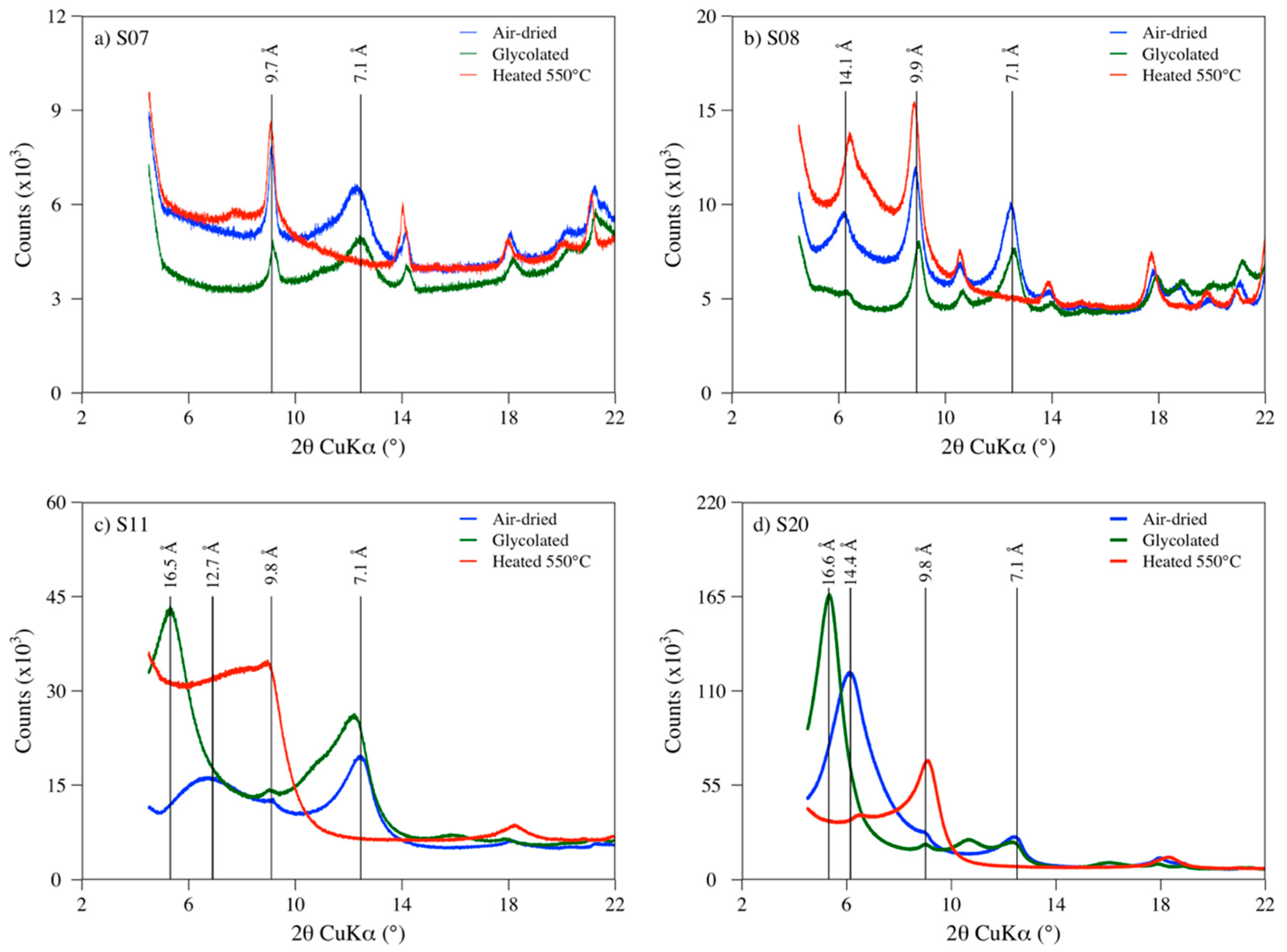
X-ray diffraction (XRD) analyses showed that the four strata have a similar mineralogical composition (Figure 3). The soil samples were mainly composed of plagioclase (Pl), quartz (Q), and potassium feldspar (Kfs), with variable amounts of amphibole type actinolite (Am), illite (I), smectite (Sm), kaolinite (Kln), and halite (Hl) (Table 3). The samples had between 8 and 22% of clay minerals. The presence of smectite was confirmed by peaks at about 14 Å in the air-dried conditions, which expanded to about 16.6 Å in ethylene glycol and collapsed at 10 Å when calcinated. Illite was identified by peaks at about 10 Å that were unaffected by ethylene glycol solvation and heating. Kaolinite minerals were observed by peaks at about 7 Å in air-dried and ethylene glycol saturated samples that disappeared in the calcinated samples (Figure 4).

Figure 3.
X-ray diffraction patterns of samples: (a) S07; (b) S08; (c) S11; and (d) S20. Note: Hl = halite, I = illite, Kfs = potassium feldspar, Kln = kaolinite, Pl = intermediate plagioclase, Q = quartz, and Sm = Smectite.
Table 3.
Mineralogical composition of the selected soil samples.

Figure 4.
X-ray diffraction patterns of clay fraction of samples: (a) S07, (b) S08, (c) S11, and (d) S20.
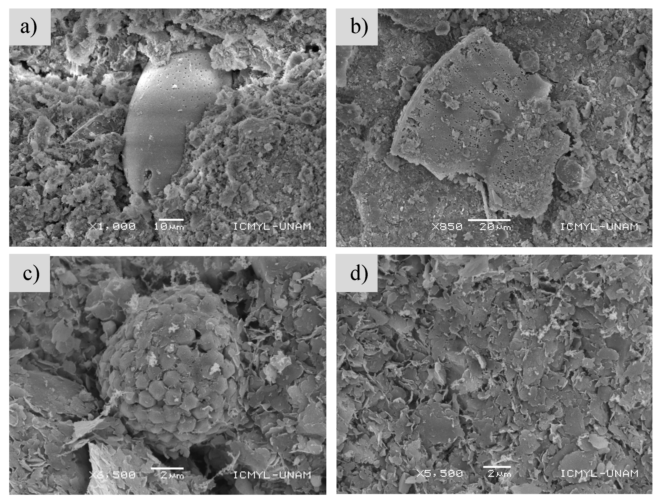
SEM micrographs from clayey samples (S07 and S11) showed the presence of microscopic organisms, diatoms, and pyrite in the forms of framboids and individual euhedral crystals (Figure 5a–c). The images also revealed that large proportions of clay particles lie parallel to the horizontal plane (Figure 5d). This preferred orientation is characteristic of a dispersed microfabric and suggests a possible anisotropy in the thermal and hydraulic properties of fine-grained strata [40].

Figure 5.
SEM micrographs of fine-grained samples (S07 and S11): (a) microscopic organism, (b) diatom frustule, (c) pyrite framboid, (d) dispersed clay microfabric.
3.2. Thermal Properties Measurements
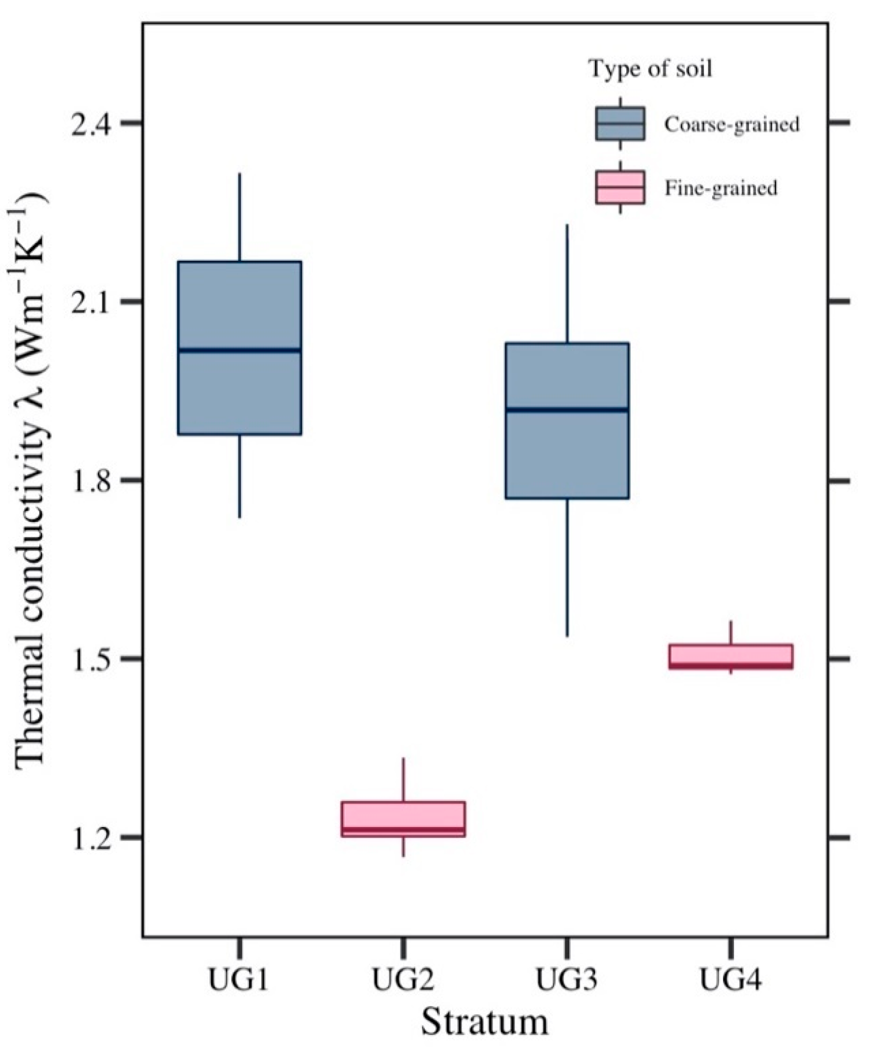
The thermal conductivity (λ) of Tabasco coastal soils varied between 1.17 and 2.32 W m−1 K−1 (Table 4) and showed no specific trend with depth. These values are relatively high and fall within the range reported in the literature for saturates soils [41]. The above may be due to the presence of minerals with high thermal conductivity (i.e., quartz, actinolite, and halite). In general, sandy soils (UG1 and UG3) had greater thermal conductivities and exhibited greater dispersions than clayey strata (UG2 and UG4) (Figure 6). To contrast this hypothesis, a one-way unbalanced analysis of variance (ANOVA) was conducted. Levene’s test indicated unequal variances for the strata (F(3,21) = 3.907, p-value = 0.023), and thus a Welch’s ANOVA [42] was selected. The results showed that there was a significant difference between the mean thermal conductivity of the four strata (F(3.68) = 49.43, p-value = 5.05 × 10⁻⁵). Post-hoc multiple comparison tests using the Games–Howell method [43] indicated that , where , , and are the mean thermal conductivity of UG2, UG3, and UG4 strata, respectively. However, the mean thermal conductivity of UG1 and UG3 strata did not differ significantly. Considering the above, the soil samples were classified into two groups for further analysis: (a) coarse-grained (UG1 and UG3), and (b) fine-grained soils (UG2 and UG4).
Table 4.
Summary statistics of thermal conductivity (λ) of Tabasco coastal soils a.

Figure 6.
Boxplot comparison of thermal conductivity of each stratum.
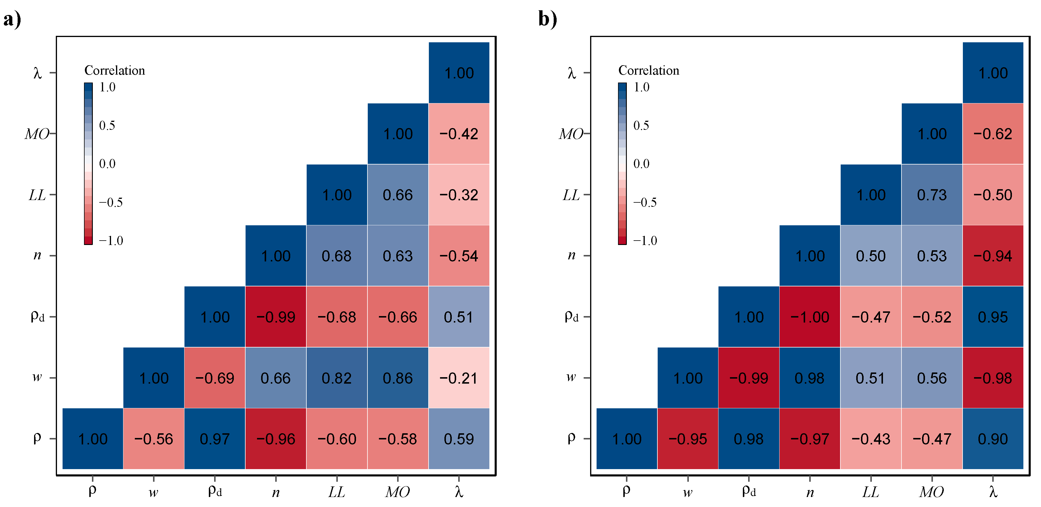
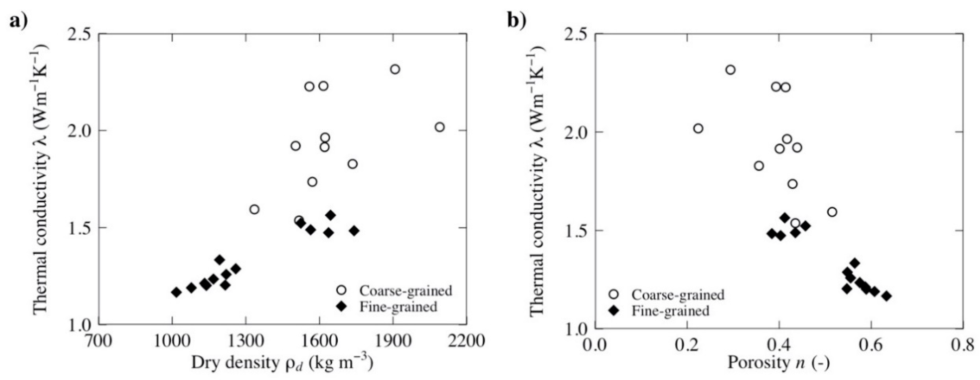
Figure 7 presents the correlation matrix between the index and thermal properties of Tabasco coastal soils. Even though both groups showed a similar trend, fine-grained soils exhibited a stronger linear relationship between their properties (Figure 8). There was a significant correlation between the thermal conductivity of these sediments and their dry density (ρd) and porosity (n). Higher thermal conductivities were associated with higher dry densities and lower porosities (Figure 8). This behavior has been reported by other authors [8,9,44] for different types of soils and has been related to an increase of solid particles per unit volume and the solid-to-solid contact points.

Figure 7.
Correlation matrix of index and thermal properties: (a) coarse-grained; and (b) fine-grained soils. Note: ρ = total density, w = water content, ρd = dry density, n = porosity, LL = liquid limit, OM = organic matter, λ = thermal conductivity.

Figure 8.
Effect of index properties on the thermal conductivity of the soil samples: (a) dry density; and (b) porosity.
3.3. Assessment of Theoretical Thermal Conductivity Models
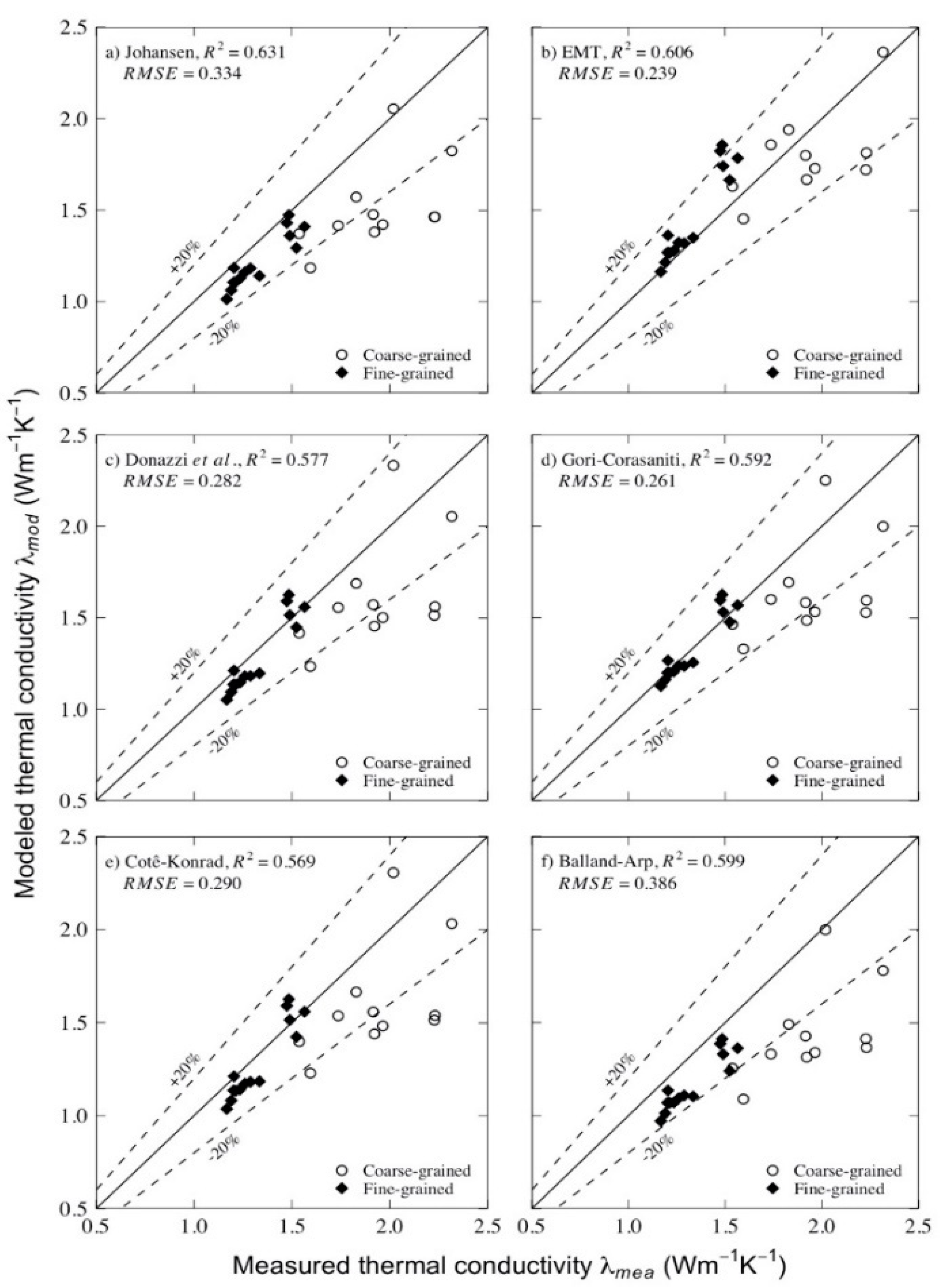
Goodness-of-fit metrics (Table 5) were similar for the six evaluated models with R2 ranging between 0.577 and 0.631 and RMSE varying between 0.239 and 0.334. However, scatter plots showed that Johansen [30] and Balland–Arp [34] models generally underestimated the measured thermal conductivity (Figure 9a,f). This discrepancy is caused by the unrealistic estimations of the thermal conductivity of soil solids (λs). Both Johansen and Balland–Arp models used a simplified version of the generalized geometric mean method that considers the thermal conductivity of non-quartz minerals equal to 2.0 W m−1 K−1, but the mineralogical analyses performed here (Section 3.1) showed that Tabasco coastal soils have minerals with higher thermal conductivities, such as actinolite (3.5 W m−1 K−1) and halite (6.1 W m−1 K−1).
Table 5.
Goodness-of-fit metrics of evaluated theoretical thermal conductivity models a.
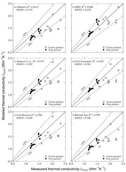
Figure 9.
Measured thermal conductivity compared with the evaluated theoretical thermal conductivity models: (a) Johansen; (b) EMT; (c) Donazzi et al.; (d) Gori–Corasaniti; (e) Cotê–Konrad; and (f) Balland–Arp.
Scatter plots (Figure 9) also revealed that the accuracy of the estimations obtained by theoretical thermal conductivity models varied depending on the type of soil. Accordingly, the R2 and RMSE were calculated for the fine- and coarse-grained soils, separately (Table 5). This analysis showed that the evaluated models provide a better agreement to the experimental data of fine-grained soils, improving in both of the statistical metrics. For this type of soils, the Gori–Corasaniti model gave the most accurate estimations with R2 = 0.89 and RMSE = 0.063. Conversely, only the EMT model provided a satisfactory fit to the measured thermal conductivity of coarse-grained soils (most estimations with an error of less than 20%). The other five models (Johansen, Donazzi et al., Gori–Corasaniti, Cotê–Konrad, and Balland–Arp) gave scatter results and tended to underestimate the thermal conductivity of the samples. The above can be attributed to the empirical nature of the evaluated model and the heterogeneity of the coarse-grained strata discussed in Section 3.1 and 3.2.
4. Conclusions
Like other countries, in Mexico, ground-source heat pump systems (GSHPs) and energy geostructure systems have been proposed as viable alternatives to reducing the environmental impact of the growing demand for space conditioning. An accurate design of these systems requires the correct estimation of some thermal properties, such as the soil’s thermal conductivity, undisturbed ground temperature, and ground heat exchanger (GHE) thermal resistance. Despite its importance, the information about the thermal properties of Mexican soils is scarce, which restrains the application of GSHPs and energy geostructures. This paper presented a comprehensive characterization of the thermal conductivity of typical coastal soils of Tabasco, Mexico, with the aim of promoting the construction of energy geostructures in the country. Twenty-five undisturbed soil samples from eleven different locations and different strata were studied in the laboratory using the thermal needle probe method. Their thermal conductivity varied between 1.17 and 2.32 W m−1 K−1 and showed no specific trend with depth. The experimental results indicated that coarse-grained soils have greater thermal conductivities and variability than fine-grained soils. It was observed that an increase in the dry density and the associated reduction of the porosity of the samples provoke an increment in their thermal conductivity.
Mineralogical analyses showed that the different soil strata have a similar composition, consisting mainly of plagioclase, quartz, and potassium feldspar, with variable amounts of amphibole type actinolite, illite, smectite, kaolinite, and halite. The presence of high thermal conductivity minerals (i.e., quartz, actinolite, and halite) explains the relatively high thermal conductivities measured in the evaluated undisturbed samples. Additionally, scanning electron microscope (SEM) images provided significant observations of the soil microstructure, revealing a dispersed microfabric and suggesting a possible anisotropy in the thermal and hydraulic properties of fine-grained strata. Finally, the measured thermal conductivities were compared with six thermal conductivity models. Most of them showed an adequate fit to the experimental data of the fine-grained soils, but only the effective medium theory (EMT) provided a reasonable agreement to the thermal conductivity of coarse-grained soils. These differences were attributed to the empirical nature of the models and the large variability of the index and thermal properties of the coarse-grained strata in the study site.
The reported values represent an invaluable resource for the implementation of GSHPs and energy geostructures in Mexico, providing new information about the thermal conductivity of local soils for the first database of this type in our country. Moreover, the presented data can serve for feasibility studies and preliminary designs of these technologies in locations and other countries with similar subsoil conditions when it is not possible to carry out experimental tests to obtain the thermal properties of soils because of lack of time or economic or material resources. Nevertheless, it must be noted that a laboratory characterization cannot replace the results of a thermal response test (TRT) performed in situ, since the latter provides additional valuable information (undisturbed ground temperature and GHE thermal resistance, in addition to the ground thermal conductivity) and evaluates larger volumes of soils under site-specific conditions that can affect the soil’s thermal properties (e.g., groundwater flow). Therefore, the authors recommend the performance of a thermal response test (TRT) for detailed and accurate borehole heat exchanger designs.
Author Contributions
Conceptualization, N.P.L.-A. and D.F.B.-G.; methodology, A.I.Z.-C.; software, D.F.B.-G.; validation, N.P.L.-A., D.F.B.-G. and A.I.Z.-C.; formal analysis, D.F.B.-G.; investigation, A.I.Z.-C.; resources, N.P.L.-A.; data curation, D.F.B.-G.; writing—original draft preparation, D.F.B.-G.; writing—review and editing, N.P.L.-A.; visualization, D.F.B.-G.; supervision, N.P.L.-A.; project administration, N.P.L.-A.; funding acquisition, N.P.L.-A. All authors have read and agreed to the published version of the manuscript.
Funding
This research received no external funding.
Acknowledgments
The authors acknowledge Teresa Pi Puig of the XRD Laboratory of The National Laboratory of Geochemistry and Mineralogy (LANGEM) of the Universidad Nacional Autónoma de México (UNAM) for determining the mineralogical composition of the soil samples, and Laura Elena Gómez Lizárraga of the Instituto de Ciencias del Mar y Limnología of UNAM for her assistance in the acquisition of SEM images.
Conflicts of Interest
The authors declare no conflict of interest.
References
- Secretaría de Energía (SENER). Balance Nacional de Energía 2017; Secretaría de Energía (SENER): Mexico City, Mexico, 2018. [Google Scholar]
- Oropeza-Perez, I.; Petzold-Rodriguez, A. Analysis of the energy use in the mexican residential sector by using two approaches regarding the behavior of the occupants. Appl. Sci. 2018, 8, 2136. [Google Scholar] [CrossRef] [Green Version]
- SENER. Electricity Sector Outlook 2016–2030; SENER: Mexico City, Mexico, 2016. [Google Scholar]
- López-Acosta, N.P.; Barba-Galdámez, D.F.; Sánchez, M. Numerical analysis of the thermo-mechanical behavior of an energy pile in Mexico. In Proceedings of the Energy Geotechnics SEG 2018, Lausanne, Switzerland, 25–28 September 2018; Ferrari, A., Laloui, L., Eds.; Springer: Cham, Switzerland, 2019; pp. 147–154. [Google Scholar]
- Loveridge, F.; Low, J.; Powrie, W. Site investigation for energy geostructures. Q. J. Eng. Geol. Hydrogeol. 2017, 50, 158–168. [Google Scholar] [CrossRef]
- Portillo-Arreguín, D.M.; López-Acosta, N.P.; Barba-Galdámez, D.F.; Rao Singh, M. Thermal Properties of Mexico Basin Soils. In Proceedings of the Geotechnical Engineering in the XXI Century: Lessons Learned and Future Challenges, Cancun, Mexico, 17–20 November 2019; López-Acosta, N.P., Martínez-Hernández, E., Espinosa-Santiago, A.L., Mendoza-Promotor, J.A., Ossa López, A., Eds.; IOS Press: Amsterdam, The Neherlands, 2019; pp. 2858–2863. [Google Scholar]
- Silva-Aguilar, O.F.; Andaverde-Arredondo, J.A.; Escobedo-Trujillo, B.A.; Benitez-Fundora, A.J. Determining the in situ apparent thermal diffusivity of a sandy soil. Rev. Bras. Ciência Solo 2018, 42, 1–13. [Google Scholar] [CrossRef] [Green Version]
- Farouki, O.T. Thermal Properties of Soils (No. CRREL-MONO-81-1); Cold Regions Research and Engineering Laboratory: Hanover, NH, USA, 1981. [Google Scholar]
- Barry-Macaulay, D.; Bouazza, A.; Singh, R.M.; Wang, B.; Ranjith, P.G. Thermal conductivity of soils and rocks from the Melbourne (Australia) region. Eng. Geol. 2013, 164, 131–138. [Google Scholar] [CrossRef] [Green Version]
- Eklöf, C.; Gehlin, S. TED—A Mobile Equipment for Thermal Response Test: Testing and Evaluation; Luleå University of Technology: Luleå, Sweden, 1996. [Google Scholar]
- Clarke, B.G.; Agab, A.; Nicholson, D. Model specification to determine thermal conductivity of soils. Proc. Inst. Civ. Eng. Geotech. Eng. 2008, 161, 161–168. [Google Scholar] [CrossRef]
- ASTM D5334-14. Standard Test Method for Determination of Thermal Conductivity of Soil and Soft Rock by Thermal Needle Probe Procedure; ASTM International: West Conshohocken, PA, USA, 2014. [Google Scholar]
- Gustafsson, S.E. Transient plane source techniques for thermal conductivity and thermal diffusivity measurements of solid materials. Rev. Sci. Instrum. 1991, 62, 797–804. [Google Scholar] [CrossRef]
- Jensen-Page, L.; Loveridge, F.; Narsilio, G.A. Thermal response testing of large diameter energy piles. Energies 2019, 12, 2700. [Google Scholar] [CrossRef] [Green Version]
- Low, J.E.; Loveridge, F.A.; Powrie, W.; Nicholson, D. A comparison of laboratory and in situ methods to determine soil thermal conductivity for energy foundations and other ground heat exchanger applications. Acta Geotech. 2015, 10, 209–218. [Google Scholar] [CrossRef]
- Vieira, A.; Alberdi-Pagola, M.; Christodoulides, P.; Javed, S.; Loveridge, F.; Nguyen, F.; Cecinato, F.; Maranha, J.; Florides, G.; Prodan, I.; et al. Characterisation of ground thermal and thermo-mechanical behaviour for shallow geothermal energy applications. Energies 2017, 10, 2044. [Google Scholar] [CrossRef] [Green Version]
- Soldo, V.; Borović, S.; Lepoša, L.; Boban, L. Comparison of different methods for ground thermal properties determination in a clastic sedimentary environment. Geothermics 2016, 61, 1–11. [Google Scholar] [CrossRef]
- Zhang, Y.; Gao, P.; Yu, Z.; Fang, J.; Li, C. Characteristics of ground thermal properties in Harbin, China. Energy Build. 2014, 69, 251–259. [Google Scholar] [CrossRef]
- Loveridge, F.; McCartney, J.S.; Narsilio, G.A.; Sanchez, M. Energy geostructures: A review of analysis approaches, in situ testing and model scale experiments. Geomech. Energy Environ. 2020, 22, 100173. [Google Scholar] [CrossRef] [Green Version]
- Shim, B.O.; Park, C.H. Ground thermal conductivity for (ground source heat pumps) GSHPs in Korea. Energy 2013, 56, 167–174. [Google Scholar] [CrossRef]
- Mikhaylova, O.; Johnston, I.W.; Narsilio, G.A. Uncertainties in the design of ground heat exchangers. Environ. Geotech. 2016, 3, 253–264. [Google Scholar] [CrossRef]
- Rees, S.W.; Adjali, M.H.; Zhou, Z.; Davies, M.; Thomas, H.R. Ground heat transfer effects on the thermal performance of earth-contact structures. Renew. Sustain. Energy Rev. 2000, 4, 213–265. [Google Scholar] [CrossRef]
- Dong, Y.; McCartney, J.S.; Lu, N. Critical review of thermal conductivity models for unsaturated soils. Geotech. Geol. Eng. 2015, 33, 207–221. [Google Scholar] [CrossRef]
- Aguilera-Martínez, M.A.; Zárate-López, J.; Barrios-Rodríguez, F.; Jiménez-Hernández, A. Carta Geológico-Minera Frontera E15-5. Tabasco y Campeche. Escala 1:250,000; Servicio Geológico Mexicano: Pachuca, Mexico, 2004. [Google Scholar]
- Zaragoza-Cardiel, A.I. Determinación Experimental de las Propiedades Térmicas e Hidráulicas del Suelo de Paraíso, Tabasco. Bachelor’s Thesis, Universidad Nacional Autónoma de México, Mexico City, Mexico, 2020. [Google Scholar]
- ASTM D2487-17. Standard Practice for Classification of Soils for Engineering Purposes (Unified Soil Classification System); ASTM International: West Conshohocken, PA, USA, 2017. [Google Scholar]
- IEEE Std 442-2017. Guide for Thermal Resistivity Measurements of Soils and Backfill Materials; IEEE Standards Association: New York, NY, USA, 2017. [Google Scholar]
- Carslaw, H.S.; Jaeger, J.C. Conduction of Heat in Solids, 2nd ed.; Oxford University Press: Oxford, UK, 1959; ISBN 0198533683. [Google Scholar]
- Jia, G.S.; Tao, Z.Y.; Meng, X.Z.; Ma, C.F.; Chai, J.C.; Jin, L.W. Review of effective thermal conductivity models of rock-soil for geothermal energy applications. Geothermics 2019, 77, 1–11. [Google Scholar] [CrossRef]
- Johansen, O. Thermal Conductivity of Soils (Draft Translation 637); Cold Regions Research and Engineering Laboratory: Hanover, NH, USA, 1977. [Google Scholar]
- Barry-Macaulay, D.; Bouazza, A.; Wang, B.; Singh, R.M. Evaluation of soil thermal conductivity models. Can. Geotech. J. 2015, 52, 1892–1900. [Google Scholar] [CrossRef]
- Dai, Y.; Wei, N.; Yuan, H.; Zhang, S.; Shangguan, W.; Liu, S.; Lu, X.; Xin, Y. Evaluation of Soil Thermal Conductivity Schemes for Use in Land Surface Modeling. J. Adv. Model. Earth Syst. 2019, 11, 3454–3473. [Google Scholar] [CrossRef]
- Côté, J.; Konrad, J.M. A generalized thermal conductivity model for soils and construction materials. Can. Geotech. J. 2005, 42, 443–458. [Google Scholar] [CrossRef]
- Balland, V.; Arp, P.A. Modeling soil thermal conductivities over a wide range of conditions. J. Environ. Eng. Sci. 2005, 4, 549–558. [Google Scholar] [CrossRef]
- Kirkpatrick, S. Percolation and conduction. Rev. Mod. Phys. 1973, 45, 574–588. [Google Scholar] [CrossRef]
- Donazzi, F.; Occhini, E.; Seppi, A. Soil thermal and hydrological characteristics in designing underground cables. Proc. Inst. Electr. Eng. 1979, 126, 506–516. [Google Scholar] [CrossRef]
- Gori, F.; Corasaniti, S. Theoretical prediction of the soil thermal conductivity at moderately high temperatures. J. Heat Transf. 2002, 124, 1001–1008. [Google Scholar] [CrossRef]
- Horai, K. Thermal conductivity of rock-forming minerals. J. Geophys. Res. 1971, 76, 1278–1308. [Google Scholar] [CrossRef]
- Brigaud, F.; Vasseur, G. Mineralogy, porosity and fluid control on thermal conductivity of sedimentary rocks. Geophys. J. Int. 1989, 98, 525–542. [Google Scholar] [CrossRef] [Green Version]
- Hicher, P.Y.; Wahyudi, H.; Tessier, D. Microstructural analysis of inherent and induced anisotropy in clay. Mech. Cohesive-Frict. Mater. 2000, 5, 341–371. [Google Scholar] [CrossRef]
- Dalla Santa, G.; Galgaro, A.; Sassi, R.; Cultrera, M.; Scotton, P.; Mueller, J.; Bertermann, D.; Mendrinos, D.; Pasquali, R.; Perego, R.; et al. An updated ground thermal properties database for GSHP applications. Geothermics 2020, 85, 101758. [Google Scholar] [CrossRef]
- Welch, B.L. On the comparison of several mean values: An alternative approach. Biometrika 1951, 38, 330. [Google Scholar] [CrossRef]
- Games, P.A.; Howell, J.F. Pairwise multiple comparison procedures with unequal N’s and/or variances: A monte carlo study. J. Educ. Stat. 1976, 1, 113–125. [Google Scholar] [CrossRef]
- Midttømme, K.; Roaldset, E.; Aagaard, P. Thermal conductivities of argillaceous sediments. Geol. Soc. Lond. Eng. Geol. Spec. Publ. 1997, 12, 355–363. [Google Scholar] [CrossRef]
Publisher’s Note: MDPI stays neutral with regard to jurisdictional claims in published maps and institutional affiliations. |
© 2021 by the authors. Licensee MDPI, Basel, Switzerland. This article is an open access article distributed under the terms and conditions of the Creative Commons Attribution (CC BY) license (https://creativecommons.org/licenses/by/4.0/).