1. Introduction
The growth of the worldwide energy demand in light of the depletion of conventional sources of energy have accelerated the urge to pursue energy-efficient systems and use of alternative energies. Buildings are responsible for nearly 40% of total electricity consumption and one-third of global gas emissions [
1]. Cooling and heating systems are among the largest energy end-users in buildings [
2,
3] and, therefore, innovative cooling and heating techniques that potentially lead to energy savings and reducing emissions are of great significance. Thermoelectric (TE) systems, as an alternative cooling/heating system, through the Peltier effect, offer several attractive characteristics including no need for refrigeration or major moving parts, quiet operation, high controllability, stability, and minimum maintenance [
4,
5,
6]. TE modules consist of n-type and p-type doped semiconductor elements that are connected thermally in parallel and electrically in series [
7]. TE modules are capable of generating power as the result of having a temperature gradient between the two sides of them (Seebeck effect) and producing a temperature gradient between the sides when supplied by DC electricity (Peltier effect). TE modules have been used in a variety of applications including cooling electronic devices [
8,
9], heat recovery [
10,
11], water treatment [
12], solar stills [
13], and thermal management of solar panels [
14,
15]. Applications of TE systems are thoroughly reviewed by Zhao and Tan [
5] and Twaha et al. [
7].
One of the emerging applications of TE systems is the use of Peltier modules for building cooling and heating, either through integration into building envelope or as separate units [
16]. Various configurations have been proposed and studied for integrated TE modules in windows [
17,
18,
19,
20] and walls [
17,
21,
22,
23,
24,
25] demonstrated promising results. A few previous studies have also been focused on incorporating TE modules in the ceiling.
The TE modules integrated into the ceiling provide means for radiant cooling. The concept is basically making a cold/hot radiating surface by lowering/increasing the surface temperature of the ceiling. The radiant ceiling panels provide thermal comfort for the occupants through radiant heat exchange between the radiating surface and the human body. Based on ASHRAE’s definition [
26], radiant ceiling panel systems are the systems for which at least half of the total heat exchange is occurring through radiation. Radiant cooling systems have received a lot of attention in recent years, owing to the advantages such as improved thermal comfort and reduced energy consumption [
27,
28,
29]. The energy performance of radiant systems in comparison with conventional systems is investigated in several studies [
30,
31,
32]. Most of the studies that have been done on radiant cooling/heating systems were focused on applications of chilled/hot water tubing behind the ceiling, and the study of thermoelectric based radiant cooling and heating systems is still in the early stages.
Lertsatitthanakorn et al. [
33,
34] investigated the performance of a TE system integrated in the ceiling for cooling purposes. They used a constant temperature heat sink and studied the impact of heat sink temperature on the performance of a TE based cooling system in a 1.5 m × 1.5 m × 2 m chamber. As expected, a lower temperature heat sink resulted in a better performance of the system. Lertsatitthanakorn et al. [
35] also looked into the thermal comfort aspects of their proposed system in the test chamber and reported that the system was capable of maintaining an indoor temperature of 27 °C with a
COP of 0.75. In a similar study by Cheng et al. [
36], a constant temperature heat sink (copper water channel) was used for the hot side of TE modules and a copper plate was used as the ceiling attached to the cold side of the TE modules. They studied the variation of
COP with water temperature by maintaining a constant input current. They showed that their new design is capable of providing an acceptable thermal comfort for the occupants. Bhargava and Najafi [
6] conducted a study to evaluate the performance of a solar-powered TE system integrated in the ceiling for space cooling and demonstrated that the system is capable of maintaining a comfort level temperature for the simulated room. The performance of a solar-powered TE based cooling and heating system integrated into the ceiling is studied by He et al. [
37]. They developed a model for both cooling and heating modes of operation and validated the results experimentally via a small apparatus for the summer season, where a
COP of 0.45 was achieved. Liu et al. [
38] proposed a solar-powered TE based system for cooling, heating, and dehumidification purposes. The TE modules were integrated into the ceiling to provide cooling for the building. They assessed the performance of the system under various input voltage, ambient temperature, and indoor temperature conditions and reported a
COP of 0.9 under operating voltage 5 V in the cooling mode and a
COP of 1.9 with an input voltage of 4 V in the heating mode. An analysis of a building envelope integrated with thermoelectric modules and radiative sky cooler is performed by [
39]. They optimized the system and achieved cooling capacity of 25.49 W/m
2 and a
COP of 2 in the presence of 1000 W/m
2 of solar irradiation and ambient temperature of 35 °C. An investigation of the dynamic thermal characteristics of thermoelectric radiant cooling panel system is conducted by Luo et al. [
40]. They developed a new system model by combining finite difference method and state-space matrix. They also used an artificial neural network for fast evaluation under dynamic conditions.
Lim et al. [
41] studied application of a phase change material layer as energy storage for a thermoelectric ceiling radiant cooling panel through numerical modeling and experiment. They showed that a 10-mm-thick PCM layer when combined with fins (>five per unit length of the panel) was the most desirable case among all cases that they studied. Duan et al. [
42] developed a model and performed a sensitivity analysis to provide a clear vision on the optimization of thermoelectric materials and how they can be improved to increase energy performance of thermoelectric cooling systems. They considered three major properties of thermoelectric modules including Seebeck coefficient, electrical conductivity, and thermal conductivity, and the results showed that
COP of cooling is a stronger function of the Seebeck coefficient.
A comprehensive review of the application of TE systems for building cooling, heating, and ventilation is conducted by Zuazua-Ros et al. [
16]. They reviewed TE based systems, integrated and non-integrated in a building envelope. More recently, a detailed review of radiative cooling systems (integrated in buildings), including thermoelectric systems, is presented by [
43]. They summarized and discussed recent applications of thermoelectric cooling systems for building applications along with other radiative cooling technologies.
Most of the previous studies indicated a strong correlation between the performance of the TE system, the input electricity, and the heat sink in use. A detailed parametric study is much needed, however, to provide insights regarding the optimal operating conditions. This becomes more important particularly when a full scale building model is in use, which is scarce in the literature.
The purpose of the present paper is to conduct a feasibility study on using TE-based cooling/heating systems for the real-world scale from an energy and economic standpoint. In this regard, the cooling and heating load of an office building located in Melbourne, FL, USA is determined via building energy simulation in eQuest. A TE-based cooling and heating system, integrated into the ceiling, is sized to satisfy the thermal loads for various operating conditions accordingly. It is assumed that the system is powered by solar PV panels. The total number of TE modules, as well as the required number of PV panels to supply the system, is evaluated for multiple input voltages and temperature gradients between the two sides of the TE modules associated with different thermal resistances. The energy performance of the system as well as the estimated savings and cost for each operating condition, are evaluated for both heating and cooling modes of operations. The results are thoroughly discussed to provide a picture regarding the energy, and cost aspects of TE based cooling and heating systems. The major practical challenges are also discussed.
2. System Description and Method
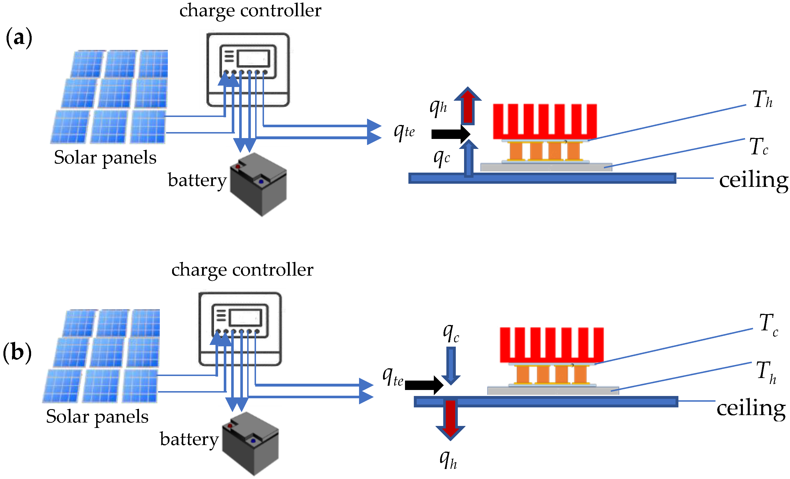
Figure 1 shows the schematic of the solar powered TE-based system integrated in the ceiling. It is considered that TE modules from the bottom side are attached to an aluminum sheet that serves as the ceiling. In hot and cold seasons, the bottom side of the TE modules cools down and heats up respectively, forming a cool/warm ceiling surface to allow the transfer of heat via radiation and convection to the occupants and provide the desired comfort level. It should be noted that by switching the direction of the electrical current supplied to TE modules the hot and cold sides of the module are switched as well. Therefore, a set of TE modules can potentially be used for both heating and cooling purposes, even though this will introduce practical challenges which will be discussed in the next section.
It is assumed that the TE modules are solar powered. PV panels are used to generate electricity. The schematic in
Figure 1 shows a possible configuration of the system which involves battery storage and charge controller. When properly sized, the system will be able to supply the TE modules with adequate electricity year-around. A more typical system with lower cost includes a charge controller, an inverter, and a net-meter that allows exporting the PV power to the grid and receive the utility power for building use (including the TE modules, after inversion to DC) simultaneously.
2.1. Methodology
The system must be sized properly to ensure the year-around occupant’s comfort. This includes the number of TE modules and PV panels to provide adequate cooling/heating and electrical power, respectively. An office building in Melbourne, FL, USA is considered for the case study and a building energy model is developed in eQuest accordingly to determine the peak hourly cooling/heating loads (Qc,max and Qh,max), as well as the yearly amount of thermal energy that must be added (Qh,y) or removed (Qc,y) to the building for maintaining desired set-point temperature.
For a given operating condition (
V and Δ
Tte), the rate of heat removal,
qc (or addition
qh) and the coefficient of performance of the TE module (
COP) are determined from the performance curves provided by the TE manufacturer. The number of required TE modules (
Nte) to meet the peak cooling/heating loads can be evaluated accordingly:
The total annual thermal energy that needs to be removed,
Qc,y, from (or added,
Qh,y, to) the building in order to maintain the desired set-point temperature are found from the building energy simulation. The total annual energy consumption by the TE modules for cooling and heating can be found as:
For simulation purposes, it is assumed that the PV panels are placed south facing (azimuth angle of 180 degrees) and at 28 degrees tilt angle (equivalent to the latitude) to maximize electricity production [
43] on the surface of the roof of a canopy that is right next to the building (south side). The PVWatts calculator [
44] is used to calculate the monthly electricity production by one panel. The number of PV panels are then calculated to cover the energy required to operate the TE modules, as described in the previous section. The number of required PV panels to provide adequate energy for the TE modules in cooling and heating modes can be then calculated as:
The performance of the proposed system and the required number of TE and PV panels are strong functions of input voltage (V) and temperature gradient between the hot and cold sides of the TE modules (ΔTte). Therefore, a parametric study is performed to compare the energy performance, required size, and cost of the system under various operating conditions.
2.2. Building Energy Model
An office building on the campus of the Florida Institute of Technology is considered for the case study. The floor area of the building is approximately 200 m
2. The exterior walls are constructed from concrete block (with a U-factor of 0.89 W/m
2 K). The roof is made of a white lacquer color on weathered asphalt pavement on a standard wood frame (U-factor 1.14 W/m
2 K). The building is occupied by six people between 8:00 a.m. to 5:00 p.m. every day except for weekends and the standard US holiday. The building energy audit was performed in order to gather all the necessary data for the building model.
Table 1 shows the list of all doors and windows and their characteristics, and
Table 2 demonstrates the list of lights and plug-loads.
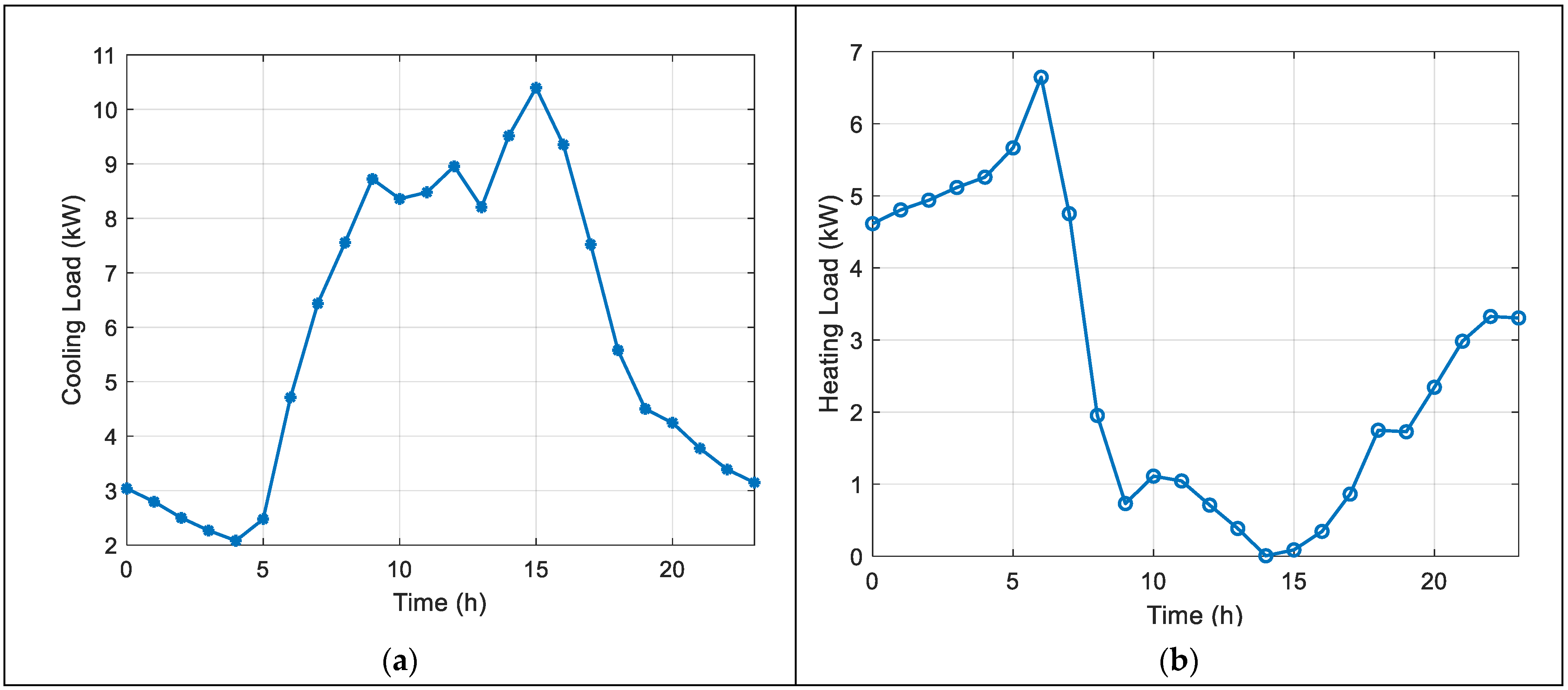
A cooling and heating set-point temperature of 298 K and 292 K are considered, respectively, for the occupied hours. The building model was developed in eQuest, and the hourly cooling/heating loads are determined for a one-year period. The highest hourly cooling and heating loads are found as 10.4 kW (Qc,max ≈ 3 tons of regrigeration) for 3:00–4:00 p.m. on 8 July and 6.74 kW (Qh,max ≈ 2 tons of refrigeration) for 7:00–8:00 a.m. on 26 January for the hot and cold seasons, respectively.
Table 3 demonstrates the characteristics of the PV panels (Panasonic 330 W panel) and thermoelectric modules (TE Technology-HP-127-1.4-1.15-71 [
45]) that are considered for this study.
For a given operating condition, including input voltage (VTE) and the temperature gradient between hot and cold sides of the module (ΔTTE), the cooling or heating effect from each module (qc or qh) as well as the corresponding coefficient of performance (COPc or COPh) can be obtained from the manufacturer performance curves. The calculation with regard to the system sizing is already described in the previous section.
3. Results and Discussion
In this section, the building energy modeling results, system sizing as well as energy and cost analysis of the system are presented and discussed in detail.
3.1. Weather Data, Cooling and Heating Load, and Solar Power
The building that is considered for simulation is in Melbourne, FL, USA. Melbourne, situated along the Atlantic coastline in central Florida, has a humid subtropical climate (climate zone 2A, according to ASHRAE). The typical meteorological year (TMY3) is used as the source of weather data for the simulation. The TMY3 contains 12-months of hourly data that represent median weather conditions in a multiyear period and therefore is considered as a typical data set that can properly represent the weather data for a given location. The schematic of the building layout as well as the 3D model built in eQuest are shown in
Figure 2.
The maximum hourly cooling and heating loads were found to occur on 8 July at 3:00 p.m.–4:00 p.m. (10.4 kW) and 26 January 7:00 a.m.–8:00 a.m. (6.74 kW), respectively. The solar radiation data and outside dry-bulb temperature for 8 July and 26 January are plotted in
Figure 3a,b. The calculated hourly cooling load and heating load for these two days are plotted in
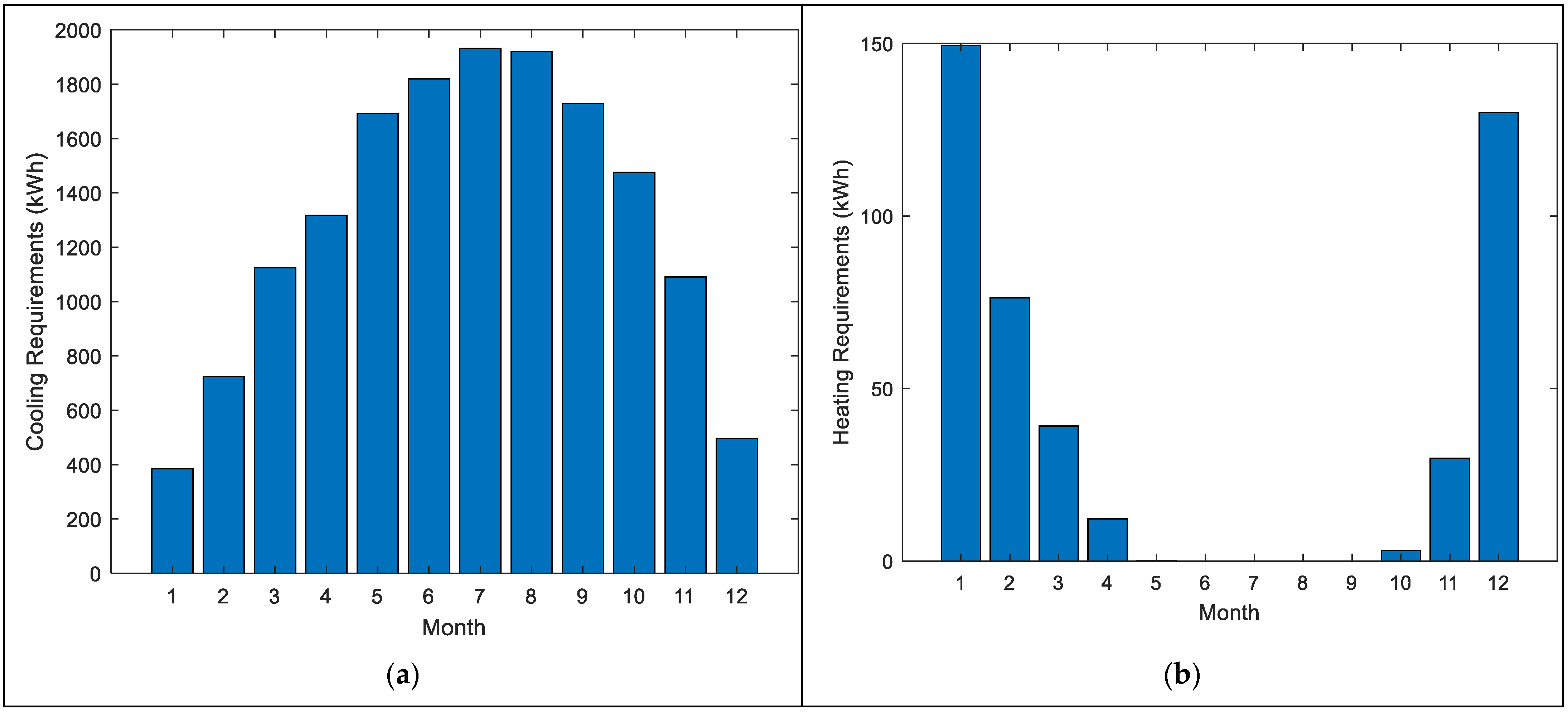
Figure 4. The total monthly heating and cooling demand of the building are calculated and demonstrated in
Figure 5.
As expected for the given hot and humid climate, the cooling load is significantly larger than the heating load, particularly for an office building with operating hours during the daytime. The highest cooling and heating demands occur in August and January, respectively. The total annual thermal energy that needs to be added/removed to/from the building in heating/cooling season to maintain the set-point temperature is found as 440 kWh and 15,707 kWh, respectively. It should be noted that this number is associated with occupied hours only, and holidays and weekends, as well as other unoccupied hours, are excluded.
The monthly electricity production by a PV panel is calculated via PVWatts calculator [
40]. It is assumed that the solar panel is placed horizontally on the roof with a tilt angle equivalent to the latitude (28 degrees). The number of required PV panels for each operating condition is found using Equation (3).
As shown in
Figure 6, the maximum electricity production is associated with May in the amount of 50.4 kWh, and the total annual electricity production is calculated as 522.7 kWh/yr.
3.2. Thermoelectric Module Performance
The performance of TE modules under various operating conditions, including input voltage (
V) and temperature gradients between hot and cold sides (Δ
Tte) is evaluated. The coefficient of performance for a TE module in cooling mode of operation may be given as:
where α,
k,
R,
Tc, and
Th represent the Seebeck coefficient, thermal conductance, electrical resistance, and cold and hot side temperature of the TE modules, respectively. In addition,
qc is the heat removal rate and
qte,c is the input electricity supplied to the TE module (for cooling), which may be defined as:
The coefficient of performance for the heating mode of operation (
COPh) assuming similar
V and Δ
Tte can be found as:
It should be noted that, as seen in Equation (4), the
COP of TE modules is a strong function of the temperature gradient between the hot and cold sides of the module (Δ
Tte). The larger Δ
Tte results in a lower coefficient of performance. Maintaining a reasonably low Δ
Tte requires effective thermal management and selection of an appropriate heat sink that provides minimum thermal resistance. The relationship between the thermal resistance on the hot/cold side of the TE module and the corresponding temperatures can be given as:
where
Ta is the ambient/surrounding temperature, and
Rth,h, and
Rth,c are the thermal resistances on the hot and cold sides of the TE module, respectively. The effect of the thermal resistances on the
COP of the TE module is further explored in
Figure 7. In this analysis, it is assumed that the thermal resistances on both sides of the TE modules are equal.
As seen, an increase in thermal resistance for a given input electrical current results in a significant reduction of COP. It is also observed that higher electricity input results in lower COP for the TE modules. These results further emphasize the importance of heat sink design and the adjustment of electricity input to the TE modules for achieving optimal performance. The detailed design of the heat sink, however, is outside the scope of the present study.
3.3. Parametric Study
The procedure for system sizing is already described in
Section 2.1. For the selected TE module, five different Δ
Tte are considered, including 9.6, 12, 19.2, 28.8, and 38.3 °C. For each particular Δ
Tte, a number of possible input voltages are considered, and the corresponding
COP, heat removal/addition rate (
qc or
qh), and energy consumed by a TE module (
qte) operating under these conditions are evaluated and listed in
Table 4. As an example, consider the first row of
Table 4, in the cooling mode operation, for Δ
Tte = 9.6 °C and
V = 2.9 V, the values of
COPc,
qc, and
qte,c are determined as 3, 14 W, and 4.67 W, respectively. Similarly, for the first row, in the heating mode operation, the values of
COPh and
qh are evaluated as 4 and 18.67 W, respectively.
Using the building energy model, the maximum cooling and heating loads (sensible and latent load) are found as 10.4 kW and 6.74 kW, respectively. The required number of TE modules for the hot and cold seasons are then calculated using Equation (1) for each operating condition. For the Δ
Tte = 9.6 °C and
V = 2.9 V (first row in
Table 4), these values are determined as 743 and 358, respectively. Note that, since the building under study is located in a hot and humid climate zone, the cooling load is much more significant than the heating load. Therefore, assuming each TE module can operate in both cooling and heating mode by switching the direction of input electricity, the system must be sized based on the cooling needs.
As mentioned, the total annual heat that must be removed and added to the building for maintaining the comfort conditions during the hot and cold seasons are found as 15,7
07 kWh and
440 kWh, respectively. These values are substituted in Equation (3) to evaluate the number of PV panels that are needed to provide sufficient electricity for the modules. For the first row of
Table 4 (Δ
Tte = 9.6 °C and V = 2.9 V), 11 PV panels are needed to provide sufficient electricity for TE modules in the cooling mode operation. In contrast, only four PV panels are required to cover the electrical energy for the TE modules in the heating mode of operation. Note that the sizing must be performed based on the cooling demands since the cooling load is significantly higher than the heating load.
It can be seen from
Table 4 that
COP values decline as the temperature gradient between the hot and cold sides increases. The performance of the TE modules can be improved if they are integrated with proper heat sinks in order to have effective heat dissipation. A closer look at the trend of the results in
Table 4 also shows that, at a given temperature gradient, for most cases, each module operates more efficiently (higher
COP) when supplied with lower input voltages. However, at lower input voltages, the heat removal/addition rate by the TE module is smaller. As a result, a more efficient cooling/heating system requires a larger number of TE modules to satisfy the load. In other words, a lower operating cost requires a higher initial investment in TE modules.
In order to provide a clearer picture of the system’s performance, the variation of
Npv and
Nte versus
COP at different temperature gradients and for various operating voltages are plotted in
Figure 8 for cooling mode of operation. It is shown that, as
COP value increases, each module provides less cooling/heating effect, and, as a result, the required number of TE modules to address the load increases, whereas the required number of PV panels decreases as the result of more efficient operation of each TE module.
An important observation can be made by reviewing the range of COP values that are obtained. For the majority of operating conditions, the COP is very small and not comparable with conventional high-efficiency heating (heat pump) and air conditioning systems. As previously discussed, a well-designed heat sink would allow efficient operation by maintaining a low ΔTte. The cases with reasonably high COP are associated with the lowest ΔTte values (9.6 °C and 12 °C). It should be noted that the COP should not be the only parameter when it comes to the energy efficiency of the proposed system. The TE based cooling/heating system allows individual control over each module, which facilitates cooling and heating based on occupancy of a certain area within each room. This will reduce the overall energy used for cooling/heating since not all the areas are always occupied.
3.4. Economic Analysis
A basic cost model is developed to provide a perspective on the economic aspects of the proposed system. The initial cost of the system, assuming the cost of instrumentation and installation is roughly 25% of the major parts, can be estimated as:
where
Cinit refers to the total initial cost of the system and
Cte and
Cpv are the price of one TE module and one PV panel, respectively. The estimated price for each TE module is
$20, and the cost of each PV panel is obtained from the manufacturer at
$300.
As mentioned, the system must be sized based on the cooling mode of operation as the cooling load is significantly higher than the heating load. The estimated initial cost of the system for each mode of operation is shown in
Figure 9.
It can be seen from
Figure 9 that case 2 (closely followed by case 5) offers the lowest initial cost of
$13,800. Case 2 demonstrated the second-highest
COP (1.7) among all the cases. A higher
COP lowers the number of required PV panels, which significantly brings the initial cost down. The second case is, therefore, selected as the optimal operating condition. It should be noted that, although the Case 1 conditions show a higher
COP, it is not cost-effective since it requires a much large number of TE modules to provide adequate cooling.
For Case 2, it is determined that 282 TE modules and 18 PV panels are needed. This is nearly 1.41 TE module (rated at 80 W) and 0.09 PV panel (rated at 330 W) per unit of area of the building, when the system operates at an approximate COP of 1.7. In other words, a nominal cooling capacity of 112.8 W and a nominal PV capacity of 31.35 W per unit area of the building is required to achieve the target goal when the system operates at the optimal condition.
Since the system is solar-powered, cost savings will be realized as the result of a reduction in the electricity bill. Assuming an average
COPHP,c of 3 and
COPHP,h of 4 for cooling and heating by a heat pump, the electricity consumption by such a system is evaluated as 5,346 kWh using Equation (10):
Assuming an average usage rate of
$0.12/kWh, the annual cost savings is found as
$641.5 using:
The installed cost of a comparable size commercial heat pump system (excluding ductwork) is approximately $5000–$6000. This indicates that, at first look, the proposed system is significantly more expensive than conventional heat pump systems with an estimated simple payback period of over 12 years. However, there are other cost considerations that need to be discussed. It is expected that the maintenance cost of the proposed system is significantly lower than the conventional air conditioning systems and they also offer a longer lifecycle. The lifespan of a conventional air conditioning unit is about 12–15 years while this value is over 20 years for the solar panels and TE modules. Accounting for the lifecycle, the payback period of using the proposed system versus conventional units can further reduce to about 8.6 years.
Additional cost savings may be achieved through the reduction of regular maintenance costs and accurate control that allows for operating the system only when the area within the coverage is occupied. Given the function of the considered building (office), many areas remain unoccupied during working hours. By automatic shut-down of the system in the unoccupied areas, significant energy/cost savings can be realized. Considering Case 2, a conservative estimate of a 25% reduction in operating hours will result in a decrease in the number of required PV panels down to 14, which will reduce the initial cost by $1875. This will bring down the payback period to just below six years. Additionally, for the economic analysis, the cost savings is calculated using an average usage rate of $0.12 which is estimated based on electricity cost in Florida. This number could be much larger in other areas which will significantly decrease the payback period.


