The Bees Algorithm Tuned Sliding Mode Control for Load Frequency Control in Two-Area Power System

Abstract

This paper proposes a design of Sliding Mode Control (SMC) for Load Frequency Control (LFC) in a two-area electrical power system. The mathematical model design of the SMC is derived based on the parameters of the investigated system. In order to achieve the optimal use of the proposed controller, an optimisation tool called the Bees Algorithm (BA) is suggested in this work to tune the parameters of the SMC. The dynamic performance of the power system with SMC employed for LFC is studied by applying a load disturbance of 0.2 pu in area one. To validate the supremacy of the proposed controller, the results are compared with those of recently published works based on Fuzzy Logic Control (FLC) tuned by Teaching–Learning-Based Optimisation (TLBO) algorithm and the traditional PID optimised by Lozi map-based Chaotic Optimisation Algorithm (LCOA). Furthermore, the robustness of SMC-based BA is examined against parametric uncertainties of the electrical power system by simultaneous changes in certain parameters of the testbed system with 40% of their nominal values. Simulation results prove the superiority and the robustness of the proposed SMC as an LFC system for the investigated power system.

1. Introduction

Modern power systems are highly nonlinear with increasing complexity in their structure. This is because of the obvious increase in the capacity with the wide dependence on different energy sources. Consequently, many issues are associated with this nonlinearity and complexity in which frequency deviation in power systems is one of the most serious problems in this field. The problem of frequency deviation is a persistent issue presents from the continuous change in the demand which accordingly requires changing the generated power in order to keep the frequency at rated value. In power systems, this process is termed Load Frequency Control (LFC) [1]. Based on the basic role of the LFC loop, the principal tasks of this service in power systems are providing the necessitated power from the generation plants operate in the system to meet the load demand variation and maintaining the interchanged power among interconnected control areas at pre-rated values. The objectives of the LFC loop which contribute to enhancing the power system stability are to assure zero steady state errors in frequency variations and the tie-line power fluctuations. This loop is also responsible for damping the overshoot and undershoot of the oscillation in frequency and exchanged power within a specified time; this depends on the capacity of the power system and the disturbance size [2].

Different control techniques based on different theories are suggested to overcome the issue of frequency regulation in power systems [3,4]. The conventional Proportional Integral Derivative (PID) is commonly employed for LFC in power systems as well as other control applications, with roughly 90% of control loops in industry are based on the conventional control approach [5]. Authors in [6] have proposed a PI controller-based Bacteria Foraging Optimisation Algorithm (PFOA) for LFC in a two-area power system. A PID controller which has its parameters tuned by Lozi map-based Chaotic Optimisation Algorithm (LCOA) and is implemented in a multi-area interconnected power system for LFC purposes is presented in [7]. A Fractional Order PID (FO-PID) design is proposed in [8] for LFC in a two-area power system with considering aspects of nonlinearities; the parameters of this controller are concurrently optimised by Gases Brownian Motion Optimisation Algorithm (BMOA). A new FOPID structure based on cascade FO-PI and FO-PD for LFC in a two-area power system is proposed in [9]. Model Predictive Control (MPC) approach is also recommended to improve the performance of power networks as an LFC system; a distributed MPC is designed and implemented in [10] for LFC in a two-area thermal-hydropower system. Pole placement scheme is equipped in a power system-based wind farms to support grid frequency control is studied in [11]. H-infinity control-based LFC in a two-area power system under deregulation policy is suggested in [12]. Internal Model Control (IMC) design for LFC in a two-area power system is investigated in [13]. Additionally, Fuzzy Logic Control (FLC) has been employed in different structures for LFC in power systems. Fuzzy PID control is proposed in [14] for frequency control in a two-area power system where the scaling factors of the proposed controller are tuned by Teaching–Learning-Based Optimisation (TLBO). Authors in [15] have suggested Fuzzy PID with filtered derivative action (Fuzzy PIDF) for LFC in the simplified Great Britain power system, and in a dual-area power system the Bees Algorithm (BA) was employed to find the optimal values of the Fuzzy PIDF parameters.

Moreover, Sliding Mode Control (SMC) has recently been successfully implemented in different areas, for example, robotic manipulator [16,17], process control [18,19], defence applications [20,21], as well as power electronics [22,23]. This is due to the broad spectrum of advantages offered by this approach, for example, robustness against parametric uncertainties and being an effective technique in non-linear systems. SMC was also considerably utilised to solve the problem of LFC in power systems. A design of sliding mode control for a single area power system is proposed in [24], this system comprises a wind turbine as a renewable energy resource. A discrete-SMC design for LFC in a four-area interconnected power system is presented in [25]. In [26], the authors have proposed SMC design for different power systems, the parameters of the controller are optimised by Particle Swarm Optimisation (PSO) and Grey Wolf Optimisation (GWO) algorithm. The author in [27] has proposed a new full order SMC method for LFC in three different power systems. Furthermore, a sliding mode controller tuned by TLBO is suggested in [28] for LFC in an unequal dual-area multi-source power system. A design of second-order integral sliding mode control employed for LFC in a two-area power system is introduced in [29]. In [30], a highly robust observer sliding mode is proposed for LFC in a three-area power integrated with two wind turbine plants. Second-order SMC combined with state estimator has recently been proposed for LFC in a two-area interconnected power system [31].

Many scholars have revealed in the literature that the SMC could solve the issue of LFC to a great extent [26,27]. It is also verified that soft computing techniques could remarkably improve the performance of controllers. Therefore, in this paper and in view of the above-said statement, an SMC design is proposed to handle the problem of LFC in an unequal two-area power system, the mathematical model of the suggested SMC is derived based on the parameters of the investigated system. A widely studied two-area interconnected power system [7,14] is considered in this work as a testbed system to examine the potentiality of the SMC as an LFC system. Moreover, as the superiority of the Bees Algorithm over other algorithms has been proved in [15], this algorithm has been selected to optimise the parameters of SMC, this is to achieve an optimal performance of the proposed controller. Integral Time Absolute Error (ITAE) is taken as an objective function to find the optimal gains of the SMC by BA. To prove the supremacy of the proposed SMC based BA, the results obtained from applying the proposed SMC-based BA are compared with those of previously published works for the same system based on Fuzzy PID tuned by TLBO presented in [14] and traditional PID-based LCOA [7]. The robustness of the SMC-BA is also verified against a wide range of parametric uncertainties of the testbed system where ten different scenarios of parametric uncertainties are investigated.

Concisely, the novelty of this work is in its proposal to apply the Bees Algorithm (BA) for tuning sliding mode control parameters implemented for load frequency control in power systems. The SMC design used in this study is simple, understandable, and applicable. Additionally, to the best of the authors’ knowledge, no previous studies have compared the performance of SMC with Fuzzy Logic Control (FLC) for LFC. It is observed from the simulation results that the BA-optimised SMC has successfully performed as a robust LFC and affords the best dynamic performance in terms of peak undershoot with fast response as compared with the other controllers.

The rest of this research is structured as follows. Section 2 presents the investigated dual-area interconnected power system. Section 3 details the proposed SMC design. Section 4 presents the suggested optimisation tool and the used objective function. Section 5 shows the main simulation results based on the proposed SMC design; it also provides a comparison with other results based on previous studies. Section 6 investigates the robustness analyses of the proposed technique towards parametric uncertainties of the testbed system. Finally, Section 7 summarises the key outcomes and suggests future works for this research.

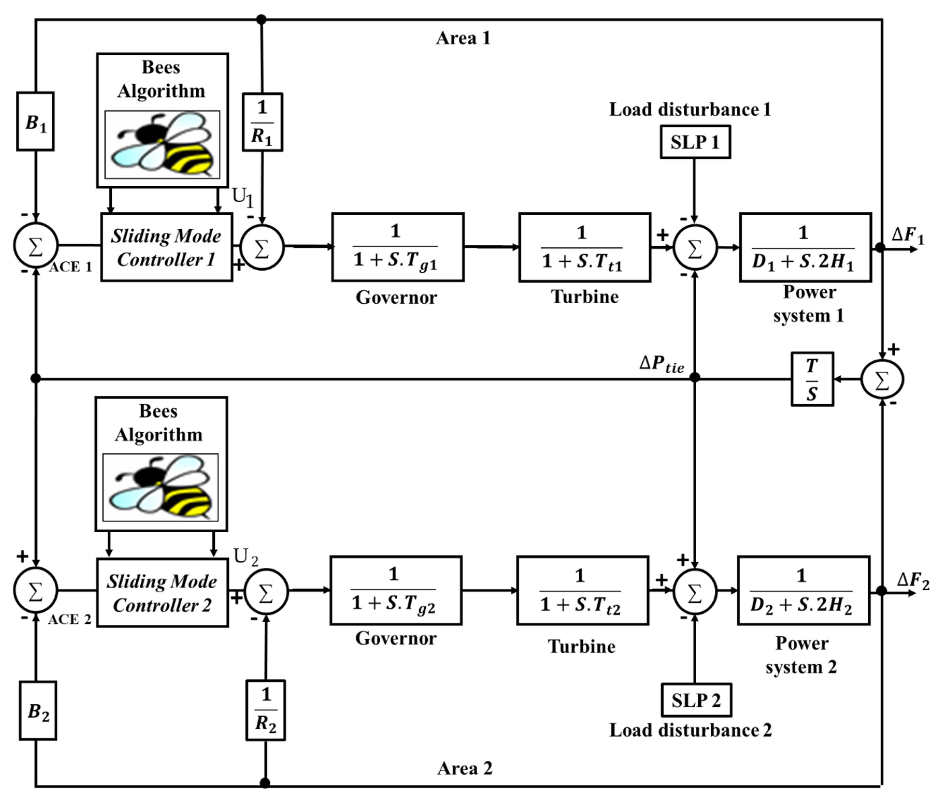
2. The Investigated Power System

The testbed model considered in this paper is shown in Figure 1. It is an extensively investigated system in literature to study the dynamic behaviour of different control concepts for LFC in power systems [7,14].

Table 1. The parameter of the testbed system [7,14].

Parameters	Definition	Values in Area 1	Values in Area 2
R	Regulation constant	0.05 MW/Hz	0.0625 MW/Hz
B	Frequency bias	20.6 Hz/MW	16.9 Hz/MW
D	The ratio of change in load to change in frequency	0.6	0.9
H	System inertia time constant	5	4
${\mathrm{T}}_{\mathrm{g}}$	Governor time constant	0.2 s	0.3 s
${\mathrm{T}}_{\mathrm{t}}$	Turbine time constant	0.5 s	0.6 s
T	Synchronization coefficient	2
F	Frequency of the system	60 Hz
SLP	Step Load Perturbation	0.2 pu

provides the associated parameters of this power system.

The term of Area Control Error (ACE) in each area is the input of the controller equipped in that area. For this system, the ACEs are represented in Equations (1) and (2).

$${\mathrm{ACE}}_{\mathrm{area} 1}=\Delta {\mathrm{P}}_{12}+{ \mathrm{B}}_1 \Delta {\mathrm{F}}_1$$

(1)

$${\mathrm{ACE}}_{\mathrm{area} 2}=\Delta {\mathrm{P}}_{21}+{ \mathrm{B}}_2 \Delta {\mathrm{F}}_2$$

(2)

where $\Delta {\mathrm{F}}_1$ and $\Delta {\mathrm{F}}_2$ are the frequency deviation in areas one and two, respectively, $\Delta {\mathrm{P}}_{12}$ and $\Delta {\mathrm{P}}_{21}$ are the power flow deviations, whilst ${\mathrm{B}}_1$ and ${\mathrm{B}}_2$ are frequency biases.

3. The Proposed Sliding Mode Control Design

The SMC follows the concept of Variable Structure Control (VSC). This approach was initially introduced at the beginning of the 1950s. Subsequently, this controller has received considerable attention from researchers, with the aim of employing it on different applications and benefiting from its numerous advantages.

The first step in designing an SMC is to identify the required behaviour of the testbed system, represented by the sliding surface of the controller. In the current research, the sliding surface of the suggested SMC design is as expressed in Equation (3):

$${\mathrm{S}\left(\mathrm{t}\right)=\mathrm{K}}_1 \ddot{\mathrm{e}}{\left(\mathrm{t}\right)+\mathrm{K}}_2{ \dot{\mathrm{e}}\left(\mathrm{t}\right)+\mathrm{K}}_3{ \mathrm{e}\left(\mathrm{t}\right)+\mathrm{K}}_4\int \mathrm{e}\left(\mathrm{t}\right) . \mathrm{dt}$$

(3)

where e(t) is the tracking error variable, ${\mathrm{K}}_1{, \mathrm{K}}_2$, ${\mathrm{K}}_3$ and ${\mathrm{K}}_4$ are the parameters that will be optimised via the Bees Algorithm. From a control perspective, it is essential to maintain the tracking signal e(t) and its derivatives equal to zero. Additionally, in order to keep S(t) at a specified value, it is required to maintain its derivative equal to zero as illustrated in (4).

$$\dot{\mathrm{S}}\left(\mathrm{t}\right)=0$$

(4)

The control law of the proposed design illustrated in (5) is selected by taking into account the condition expressed in Equations (3) and (4).

$$\mathrm{U}\left(\mathrm{t}\right){=\mathrm{U}}_{\mathrm{C}}\left(\mathrm{t}\right)+{ \mathrm{U}}_{\mathrm{D}}\left(\mathrm{t}\right)$$

(5)

where ${\mathrm{U}}_{\mathrm{C}}\left(\mathrm{t}\right)=\mathrm{F} \left(\mathrm{x}\right(\mathrm{t}), \mathrm{r}(\mathrm{t}), \mathrm{e}(\mathrm{t}\left)\right);$ in which x(t) is the control signal, r(t) is the reference signal, and e(t) is the error signal. The term ${\mathrm{U}}_{\mathrm{D}}\left(\mathrm{t}\right)$ can be expressed as in Equation (6).

$${\mathrm{U}}_{\mathrm{D}}\left(\mathrm{t}\right){=\mathrm{K}}_{\mathrm{D}} \frac{\mathrm{S}\left(\mathrm{t}\right)}{\left|\mathrm{S}\left(\mathrm{t}\right)\right|+\mathsf{\delta }}$$

(6)

where the gains ${\mathrm{K}}_{\mathrm{D}}$ and $\mathsf{\delta }$ are to be optimised by BA. Accordingly, the proposed SMC design comprises six parameters. The optimal values of these parameters are found by the BA via minimizing the integral time absolute error of the deviation in the frequency and exchanged power.

In the system shown in Figure 1, the transfer function of area one from the control signal ${\mathrm{U}}_1$ to $\Delta {\mathrm{F}}_1$ with consideration of the droop characteristic ${\mathrm{R}}_1$ can be demonstrated as in Equation (7).

$$\mathrm{G}\left(\mathrm{s}\right)=\frac{\mathrm{X} \left(\mathrm{s}\right)}{{\mathrm{U}}_{\mathrm{C}}\left(\mathrm{s}\right)}=\frac{1}{{(\mathrm{T}}_{\mathrm{g}1}{\mathrm{S}+1) (\mathrm{T}}_{\mathrm{t}1}{\mathrm{S}+1) (2 \mathrm{H}}_1{\mathrm{S}+\mathrm{D}}_1{)+1 / \mathrm{R}}_1}$$

(7)

By considering the values of the parameters tabulated in Table 1, Equation (7) can be re-written as follows:

$$\mathrm{G}\left(\mathrm{s}\right)=\frac{\mathrm{X} \left(\mathrm{s}\right)}{{\mathrm{U}}_{\mathrm{C}}\left(\mathrm{s}\right)}=\frac{1}{{\mathrm{S}}^3+ 7.06{ \mathrm{S}}^2+ 10.42 \mathrm{S}+ 20.6}$$

(8)

Equation (8) can also be written in differential form as expressed in (9)

$${\mathrm{U}}_{\mathrm{C}}\left(\mathrm{t}\right)=\stackrel{⃛}{\mathrm{x}}\left(\mathrm{t}\right) + 7.06 \ddot{\mathrm{x}}\left(\mathrm{t}\right) + 10.42 \dot{\mathrm{x}}\left(\mathrm{t}\right) + 20.06$$

(9)

From (3), Equation (4) can be re-written as follows:

$$\dot{\mathrm{S}}\left(\mathrm{t}\right)={\mathrm{K}}_1 \stackrel{⃛}{\mathrm{e}}\left(\mathrm{t}\right) +{ \mathrm{K}}_2 \ddot{\mathrm{e}}\left(\mathrm{t}\right) +{ \mathrm{K}}_3 \dot{\mathrm{e}}\left(\mathrm{t}\right) +{ \mathrm{K}}_4\mathrm{e}\left(\mathrm{t}\right)=0$$

(10)

By solving Equation (9) for the third derivative order, Equation (11) is obtained.

$${ \stackrel{⃛}{\mathrm{x}}\left(\mathrm{t}\right)=\mathrm{U}}_{\mathrm{C}}\left(\mathrm{t}\right) - 7.06 \ddot{\mathrm{x}}\left(\mathrm{t}\right) - 10.42 \dot{\mathrm{x}}\left(\mathrm{t}\right) - 20.06$$

(11)

As the variable e(t) is defined as the difference between the reference signal r(t) and the control signal x(t), this can be mathematically expressed as in (10).

$$\mathrm{e}\left(\mathrm{t}\right)=\mathrm{r}\left(\mathrm{t}\right) - \mathrm{x} \left(\mathrm{t}\right)$$

(12)

By analysing Equation (11) based on (12) and substituting the expression in (10), Equation (13) is obtained.

$$\dot{\mathrm{S}}\left(\mathrm{t}\right)=\left[\begin{array}{c}{ \mathrm{K}}_1\left[-{\mathrm{U}}_{\mathrm{C}}\left(\mathrm{t}\right) + 7.06 \ddot{\mathrm{x}}\left(\mathrm{t}\right) + 10.42 \dot{\mathrm{x}}\left(\mathrm{t}\right) + 20.06\right]\\ -{ \mathrm{K}}_2 \ddot{\mathrm{x}}\left(\mathrm{t}\right) -{ \mathrm{K}}_3 \dot{\mathrm{x}}\left(\mathrm{t}\right) -{ \mathrm{K}}_4 \mathrm{x}\left(\mathrm{t}\right)=0\end{array}\right]$$

(13)

The term ${\mathrm{U}}_{\mathrm{C}}\left(\mathrm{t}\right)$ can be identified as follows:

$${\mathrm{U}}_{\mathrm{C}}\left(\mathrm{t}\right)=\ddot{\mathrm{x}}\left(\mathrm{t}\right) [7.06-\frac{{\mathrm{K}}_2}{{\mathrm{K}}_1}] + \dot{\mathrm{x}}\left(\mathrm{t}\right) [10.42-\frac{{\mathrm{K}}_3}{{\mathrm{K}}_1}] + \mathrm{x}\left(\mathrm{t}\right) [20.6 -\frac{{\mathrm{K}}_4}{{\mathrm{K}}_1} ]$$

(14)

The control law of the controller employed in area one is expressed as in (15).

$$\begin{array}{cc}\mathrm{U}\left(\mathrm{t}\right)=& \begin{array}{c}\begin{array}{c}\ddot{\mathrm{x}}\left(\mathrm{t}\right)\left[7.06-\frac{{\mathrm{K}}_2}{{\mathrm{K}}_1}\right]+\\ \dot{\mathrm{x}} \left(\mathrm{t}\right)\left[10.42-\frac{{\mathrm{K}}_3}{{\mathrm{K}}_1}\right]+\end{array}\\ \begin{array}{c}\mathrm{x}\left(\mathrm{t}\right) \left[20.6 -\frac{{\mathrm{K}}_4}{{\mathrm{K}}_1}\right]+\end{array}\end{array}\\ & {\mathrm{K}}_{\mathrm{D}1}\left[\frac{-{\mathrm{K}}_1\ddot{\mathrm{x}}\left(\mathrm{t}\right) -{ \mathrm{K}}_2 \dot{\mathrm{x}} \left(\mathrm{t}\right) -{ \mathrm{K}}_3 \mathrm{x}\left(\mathrm{t}\right) -{ \mathrm{K}}_4\int \mathrm{x}\left(\mathrm{t}\right) . \mathrm{dt}}{\left|-{\mathrm{K}}_1\ddot{\mathrm{x}}\left(\mathrm{t}\right) -{ \mathrm{K}}_2 \dot{\mathrm{x}} \left(\mathrm{t}\right) -{ \mathrm{K}}_3 \mathrm{x}\left(\mathrm{t}\right) -{ \mathrm{K}}_4\int \mathrm{x}\left(\mathrm{t}\right) . \mathrm{dt}\right| + {\mathsf{\delta }}_1}\right]\end{array}$$

(15)

Similarly, to derive the control law of the SMC equipped in area two, the same procedure is followed, this yields the equation expressed in (16).

$$\begin{array}{cc}\mathrm{U}\left(\mathrm{t}\right)=& \begin{array}{c}\begin{array}{c}\ddot{\mathrm{x}}\left(\mathrm{t}\right)\left[7.362-1.44\times \frac{{\mathrm{K}}_6}{{\mathrm{K}}_5}\right]+\\ \dot{\mathrm{x}} \left(\mathrm{t}\right)\left[8.810-1.44\times \frac{{\mathrm{K}}_7}{{\mathrm{K}}_5}\right]+\end{array}\\ \begin{array}{c}\mathrm{x}\left(\mathrm{t}\right) \left[16.90 -1.44\times \frac{{\mathrm{K}}_8}{{\mathrm{K}}_5}\right]+\end{array}\end{array}\\ & {\mathrm{K}}_{\mathrm{D}2}\left[\frac{-{\mathrm{K}}_5\ddot{\mathrm{x}}\left(\mathrm{t}\right) -{ \mathrm{K}}_6 \dot{\mathrm{x}} \left(\mathrm{t}\right) -{ \mathrm{K}}_7 \mathrm{x}\left(\mathrm{t}\right) -{ \mathrm{K}}_8\int \mathrm{x}\left(\mathrm{t}\right) . \mathrm{dt}}{\left|-{\mathrm{K}}_5\ddot{\mathrm{x}}\left(\mathrm{t}\right) -{ \mathrm{K}}_6 \dot{\mathrm{x}} \left(\mathrm{t}\right) -{ \mathrm{K}}_7 \mathrm{x}\left(\mathrm{t}\right) -{ \mathrm{K}}_8\int \mathrm{x}\left(\mathrm{t}\right) . \mathrm{dt}\right| + {\mathsf{\delta }}_2}\right]\end{array}$$

(16)

4. The Proposed Optimisation Technique and Objective Function

It is proved that in order to enhance the performance of a controller, it is essential to understand the behaviour of the controlled plant and design the controller based on the desired behaviour of that system. Notably, one of the most important steps that plays a crucial role in the control design procedure is to find the optimal values of its parameters. However, in many cases, it is difficult to estimate the optimum values of the controller’s parameters that lead to the optimal performance. The trial-and-error technique is considerably used to overcome this matter; however, it is time-consuming and no accurate results are guaranteed. Therefore, optimisation algorithms are introduced to solve this problem to a great extent as well as other optimisation problems.

As it is explained above, in the proposed SMC design, twelve parameters will be tuned, namely: ${\mathrm{K}}_1{, \mathrm{K}}_2{, \mathrm{K}}_3{, \mathrm{K}}_4{, \mathrm{K}}_{\mathrm{D}1}{, \mathrm{and} \mathsf{\delta }}_1$ for the LFC controller equipped in area one, ${\mathrm{K}}_5{, \mathrm{K}}_6{, \mathrm{K}}_7{, \mathrm{K}}_8{, \mathrm{K}}_{\mathrm{D}2}{, \mathrm{and} \mathsf{\delta }}_2$ for the LFC controller employed in area two. These parameters are to be tuned by a metaheuristic algorithm inspired by the foraging behaviour of honeybees known as the Bees Algorithm (BA) [32]. Since its first introduction in 2005 by Professor Pham et al., this algorithm has been widely proposed by many researchers as a powerful optimisation tool to solve several problems in different fields. This is due to the wide spectrum of advantages such as simplicity and efficaciousness [33,34,35,36,37].

The algorithm requires a number of parameters to be set, specifically: number of scout bees (n), number of sites selected for exploitation out of the n visited sites (m), number of top-rated (elite) sites among the m selected sites (e), number of bees recruited for the best e sites (nep), number of bees recruited for the other (m-e) selected sites (nsp), initial size of each patch (ngh) “a patch is a region in search space that includes a visited site and its neighbourhood”, and stopping criterion.

The simplest pseudo-code for this algorithm is shown in Figure 2. The mechanism of this algorithm begins with placing the n scout bees randomly in the search space. In step 2, the evaluation of the fitness of sites visited by the n scout bees is done. The m sites with the highest fitness in specified “chosen sites” in step 3 are selected for neighbourhood or local search. The algorithm in steps 4 and 5 conducts searches in the neighbourhood of the selected sites, with more bees assigned to the best e sites. Selection of the best sites could be conducted directly based on the fitness associated with them. Alternatively, using the fitness values, the probability of sites being selected is determined. Searches in the neighbourhood of the best e sites which represent the most promising solutions are made more prominent by recruiting more bees for them than for the other selected sites. Together with scouting, this differential recruitment is a key operation of the Bees Algorithm. For each patch, only the one bee that has found the site with the highest fitness (the “fittest” bee) is selected in step 5 to form part of the next bee population. In steps 6–8, the remaining bees in the population n are assigned randomly around the search space to scout for potential new solutions or to conduct the global search. These eight steps are repeated until a stopping criterion is met. The colony will have two parts to its new population at the end of each iteration: representatives from each selected patch and other scout bees assigned to conduct random searches [38].

In this work, the parameters of the BA are set as illustrated in

Table 2. The parameters of the proposed BA.

n	m	e	nep	nsp	ngh
30	12	6	11	7	0.011

. The number of iterations was set as 100.

Furthermore, in control theories, it is always preferred to obtain a fast response combined with stability for the controlled plant. However, it is a challenging task to meet the requirements of both conditions simultaneously. Therefore, control engineering designers tend to compromise and find a balance between quick response and the required stability. This compromise can be achieved by the appropriate selection of the controller and designing it by minimising a properly specified objective function with the support of an optimisation method. In this research, the parameters of SMC proposed for LFC in the dual-area power system is optimised using the BA by minimising the Integral Time Absolute Error (ITAE) objective function expressed in Equation (17).

$$\mathrm{Objective} \mathrm{Function}=\mathrm{ITAE}={{\displaystyle \int }}_0^{\mathrm{t}}\left(\left|\Delta {\mathrm{F}}_1\right|+\left|\Delta {\mathrm{F}}_2\right|+\left|\Delta {\mathrm{P}}_{\mathrm{tie}}\right|\right).\mathrm{t}. \mathrm{dt}$$

(17)

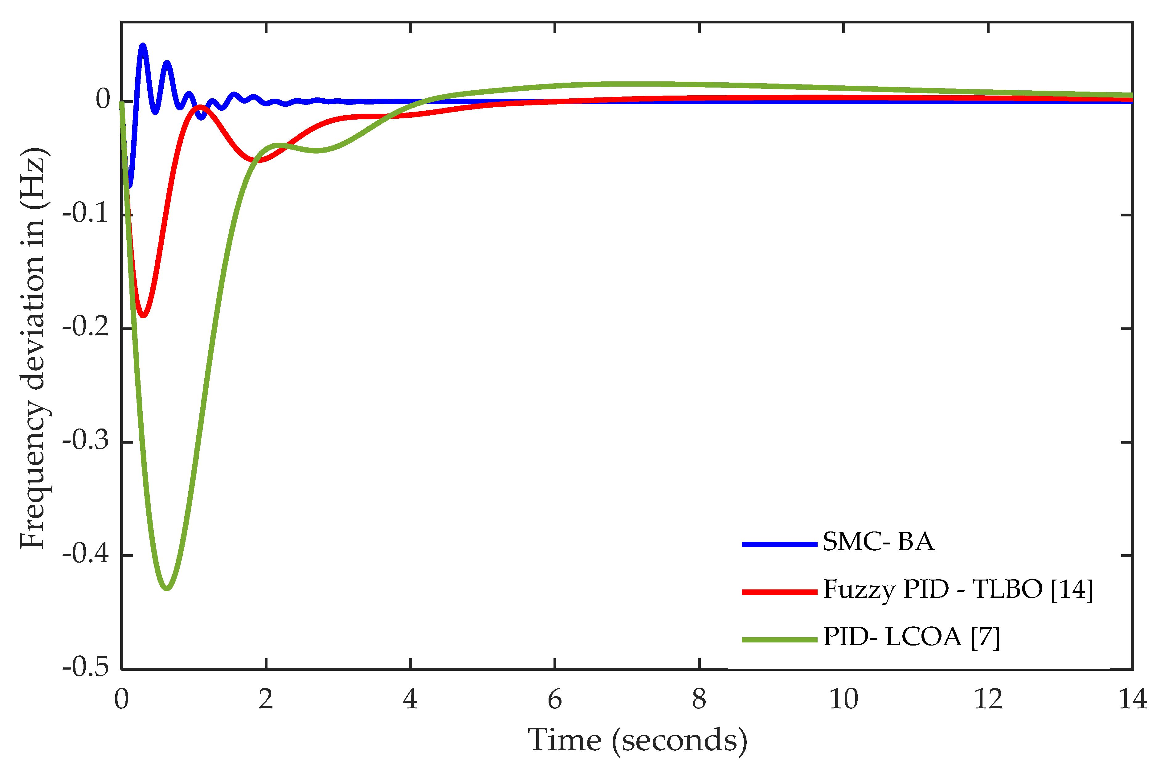
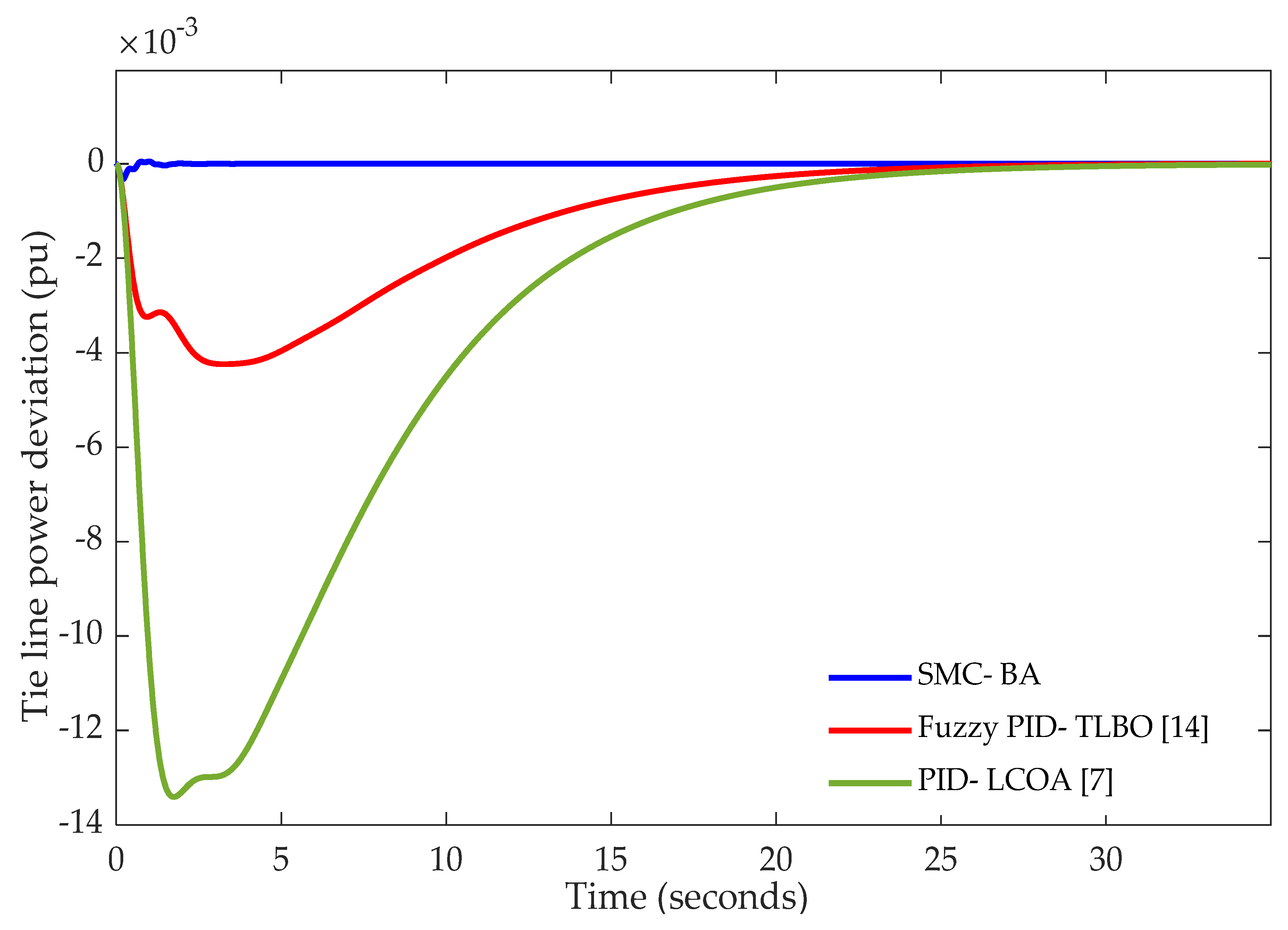
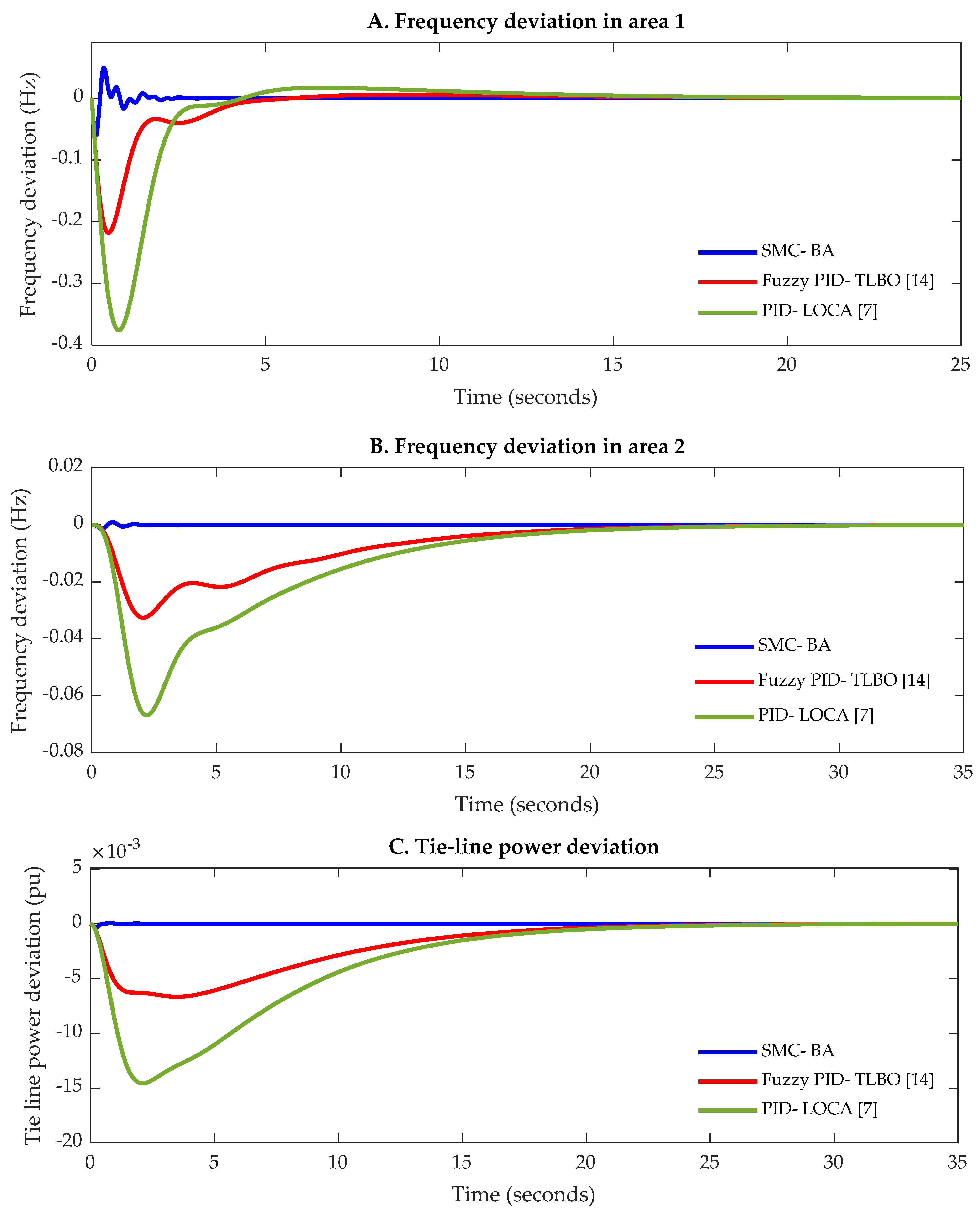
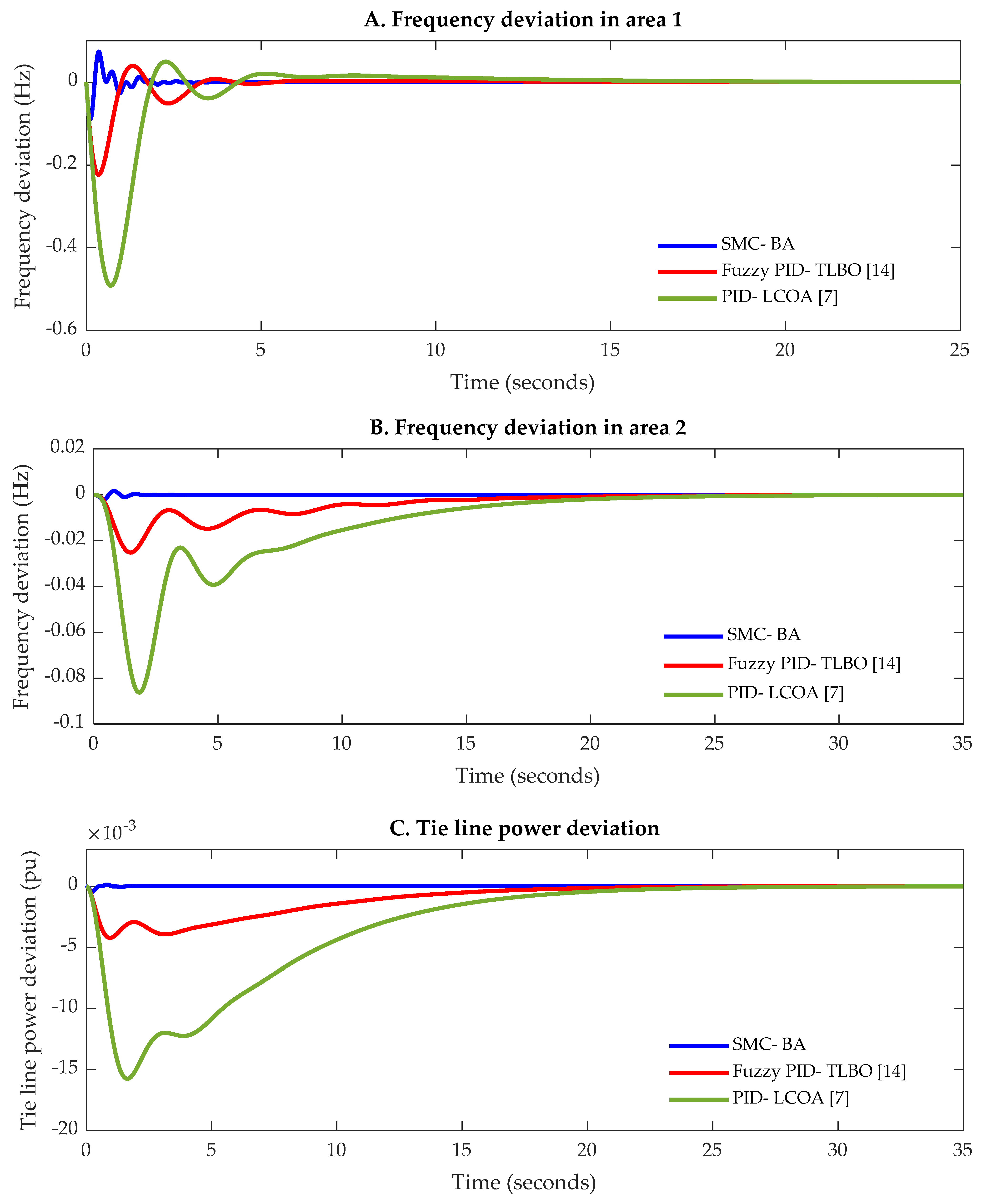
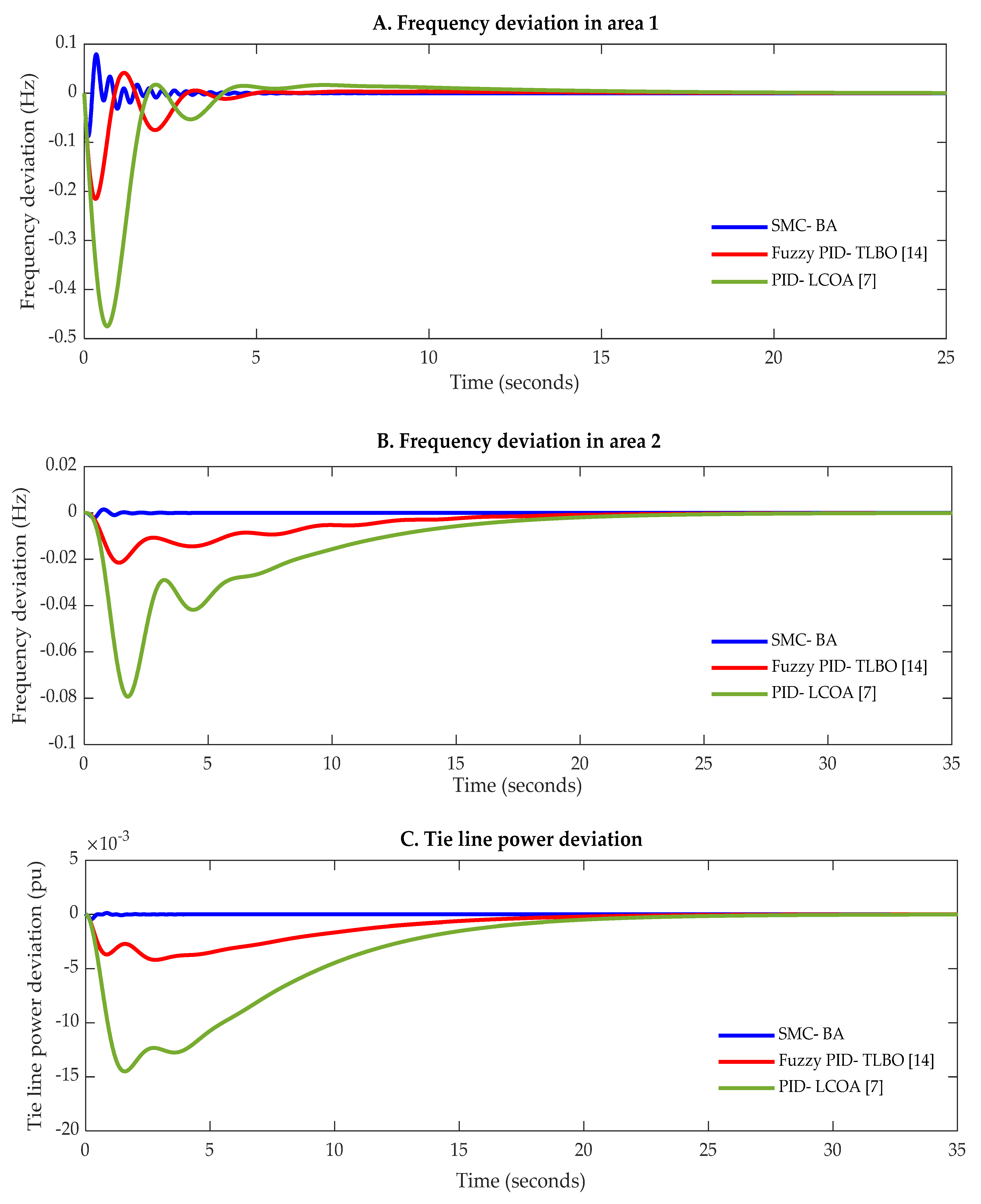
5. Results and Discussion

In this paper, a step load disturbance of 0.2 pu is applied in area one to study the dynamic performance of the testbed system when the proposed SMC tuned by BA is equipped in the system for LFC. The BA is run for 100 iterations to obtain the optimal values of the SMC parameters and the restrains of the search space is set from [0 to 2]. The optimum gains of the SMC obtained by BA are shown in

Table 3. The optimum SMC gains obtained by BA.

Controller	Parameters
SMC	Controller gains of area 1
	${\mathrm{K}}_1$	${\mathrm{K}}_2$	${\mathrm{K}}_3$	${\mathrm{K}}_4$	${\mathrm{K}}_{\mathrm{D}1}$	${\mathsf{\delta }}_1$
	1.4921	0.0309	0.1353	1.9007	1.7275	0.0029
	Controller gains of area 2
	${\mathrm{K}}_5$	${\mathrm{K}}_6$	${\mathrm{K}}_7$	${\mathrm{K}}_8$	${\mathrm{K}}_{\mathrm{D}2}$	${\mathsf{\delta }}_2$
	1.8411	1.9269	0.8824	1.8353	0.0560	1.5275

.

Furthermore, in order to demonstrate the superiority of the SMC, the results obtained are compared with those from published articles based on TLBO tuned Fuzzy PID presented in [14] and LCOA tuned traditional PID presented in [7] employed for LFC in the same system. The optimum gains of these controllers are depicted in

Table 4. The optimum gains of the controllers proposed in [7,14].

Controller	Controller Gains of Area 1				Controller Gains of Area 2
Fuzzy PID [14]	${\mathrm{K}}_1$	${\mathrm{K}}_2$	${\mathrm{K}}_3$	${\mathrm{K}}_4$	${\mathrm{K}}_5$	${\mathrm{K}}_6$	${\mathrm{K}}_7$	${\mathrm{K}}_8$
	1.9857	1.9968	1.687	1.9876	1.3469	1.5512	0.809	0.5043
PID [7]	${\mathrm{K}}_{\mathrm{P}1}$	${\mathrm{K}}_{\mathrm{I}1}$		${\mathrm{K}}_{\mathrm{D}1}$	${\mathrm{K}}_{\mathrm{P}2}$	${\mathrm{K}}_{\mathrm{I}2}$		${\mathrm{K}}_{\mathrm{D}2}$
	0.939	0.7998		0.5636	0.5208	0.4775		0.708

.

The frequency variation in area one, frequency variation in area two, and tie-line power variation following the sudden 0.2 pu disturbance applied in area one are shown in Figure 3, Figure 4 and Figure 5, respectively. From Figure 3, Figure 4 and Figure 5, it is found that the SMC tuned by BA employed for LFC in the dual-area power system offers a better dynamic response compared with those provided in [7,14]. The undershoot $\left({\mathrm{U}}_{\mathrm{sh}}\right)$, overshoot $\left({\mathrm{O}}_{\mathrm{sh}}\right),$ and settling time $\left({\mathrm{T}}_{\mathrm{s}}\right)$ of the frequency in both areas and tie-line power along with the values of the objective function are illustrated in

Table 5. Frequency response performances with different controllers.

Controller	Frequency in Area 1			Frequency in Area 2			Tie Line Power Deviation			ITAE
	${\mathbf{U}}_{\mathbf{sh}}\mathbf{in} \mathbf{Hz}$	${\mathbf{O}}_{\mathbf{sh}}\mathbf{in} \mathbf{Hz}$	${\mathbf{T}}_{\mathbf{s}} \mathbf{in} \mathbf{s}$	${\mathbf{U}}_{\mathbf{sh}}\mathbf{in} \mathbf{Hz}$	${\mathbf{O}}_{\mathbf{sh}}\mathbf{in} \mathbf{Hz}$	${\mathbf{T}}_{\mathbf{s}} \mathbf{in} \mathbf{s}$	${\mathbf{U}}_{\mathbf{sh}}\mathbf{in} \mathbf{pu}$	${\mathbf{O}}_{\mathbf{sh}}\mathbf{in} \mathbf{pu}$	${\mathbf{T}}_{\mathbf{s}} \mathbf{in} \mathbf{s}$
SMC-BA	−0.0746	0.0495	2.323	−0.0016	0.0005	2.469	−0.0003	0.00005	2.0377	0.0003
Fuzzy PID-TLBO	−0.1885	0.0035	4.9849	−0.0190	0	25.0325	−0.0042	0	24.748	0.3305
PID-LCOA	−0.4288	0.0154	11.795	−0.0664	0	21.6623	−0.0134	0	22.689	0.7920

.

From Table 5, it is observed that the settling time and undershoot of $\Delta {\mathrm{F}}_1, \Delta {\mathrm{F}}_2, \mathrm{and} \Delta {\mathrm{P}}_{\mathrm{tie}}$ is less when the proposed SMC tuned by BA is used as an LFC controller to study the dynamic behaviour of the two-area power model as compared with the other techniques studied in [7,14]. It is also evident that the value of the objective function (ITAE) is extremely less for BA-optimised SMC in comparison with the other controllers. However, a negligible increase in the overshoot is noticed.

Based on the characteristics provided in Table 5, the percentage of improvement in ${\mathrm{U}}_{\mathrm{sh}}, {\mathrm{T}}_{\mathrm{s}}, \mathrm{and} \mathrm{ITAE}$ for the SMC proposed in this research and Fuzzy PID controllers [14] in comparison with the LCOA-based PID controller [7] is shown in Figure 6. From Figure 6, it is observed that with BA-optimised SMC, undershoot and settling time in the frequency deviation of area one $\left(\Delta {\mathrm{F}}_1\right)$ are improved by 82.60% and 80.3055%, respectively. While in ($\Delta {\mathrm{F}}_2$), the undershoot and settling time in frequency deviation are improved by 97.59% and 88.606%, respectively, and in ($\Delta {\mathrm{P}}_{\mathrm{tie}}$) they are improved by 97.76% and 91.01%, respectively. Based on the results shown in Figure 3, Figure 4, Figure 5 and Figure 6 and Table 5, it is confirmed that the proposed SMC design offers the fastest response with the minimum undershoot, which in turn guarantees the best stability.

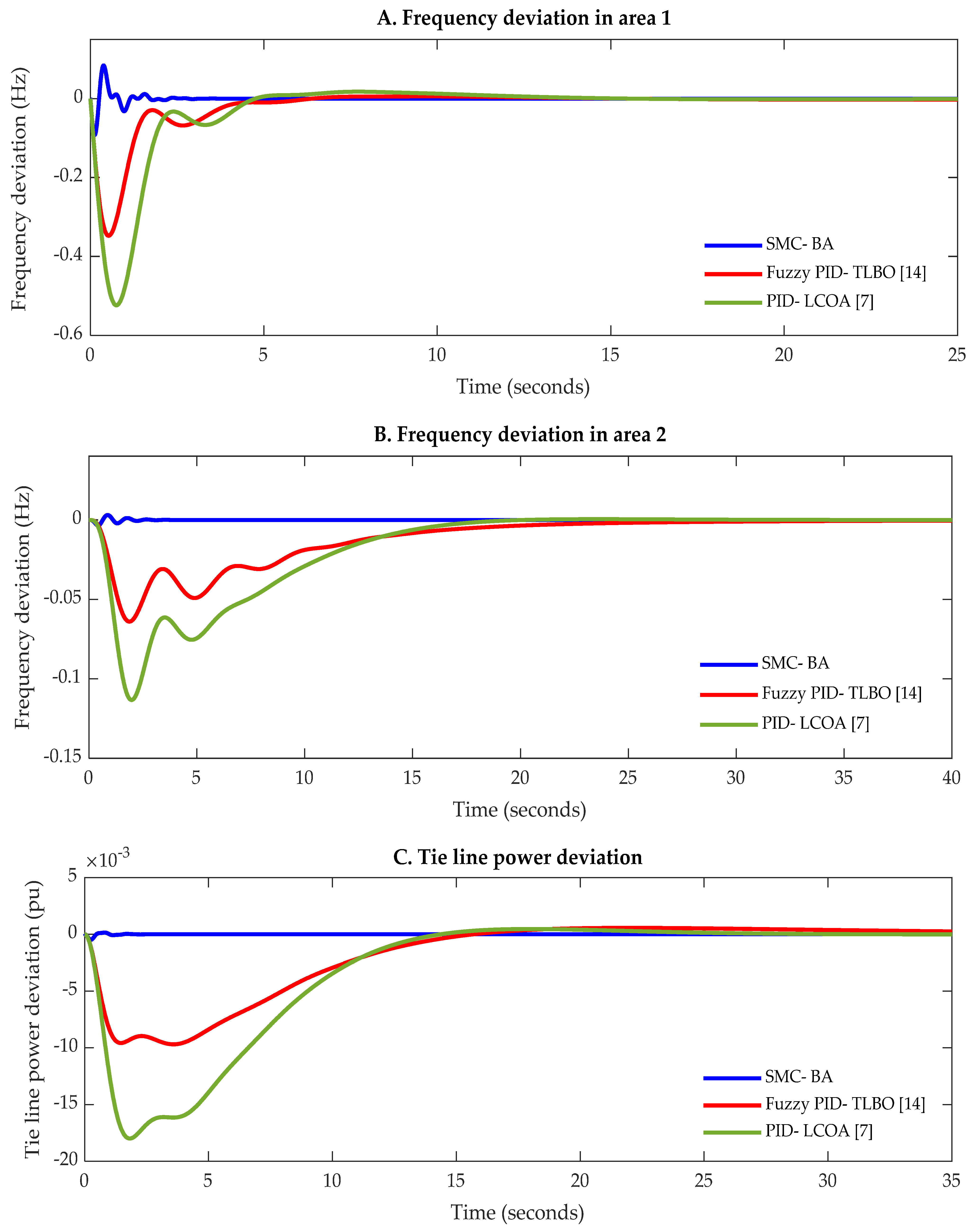
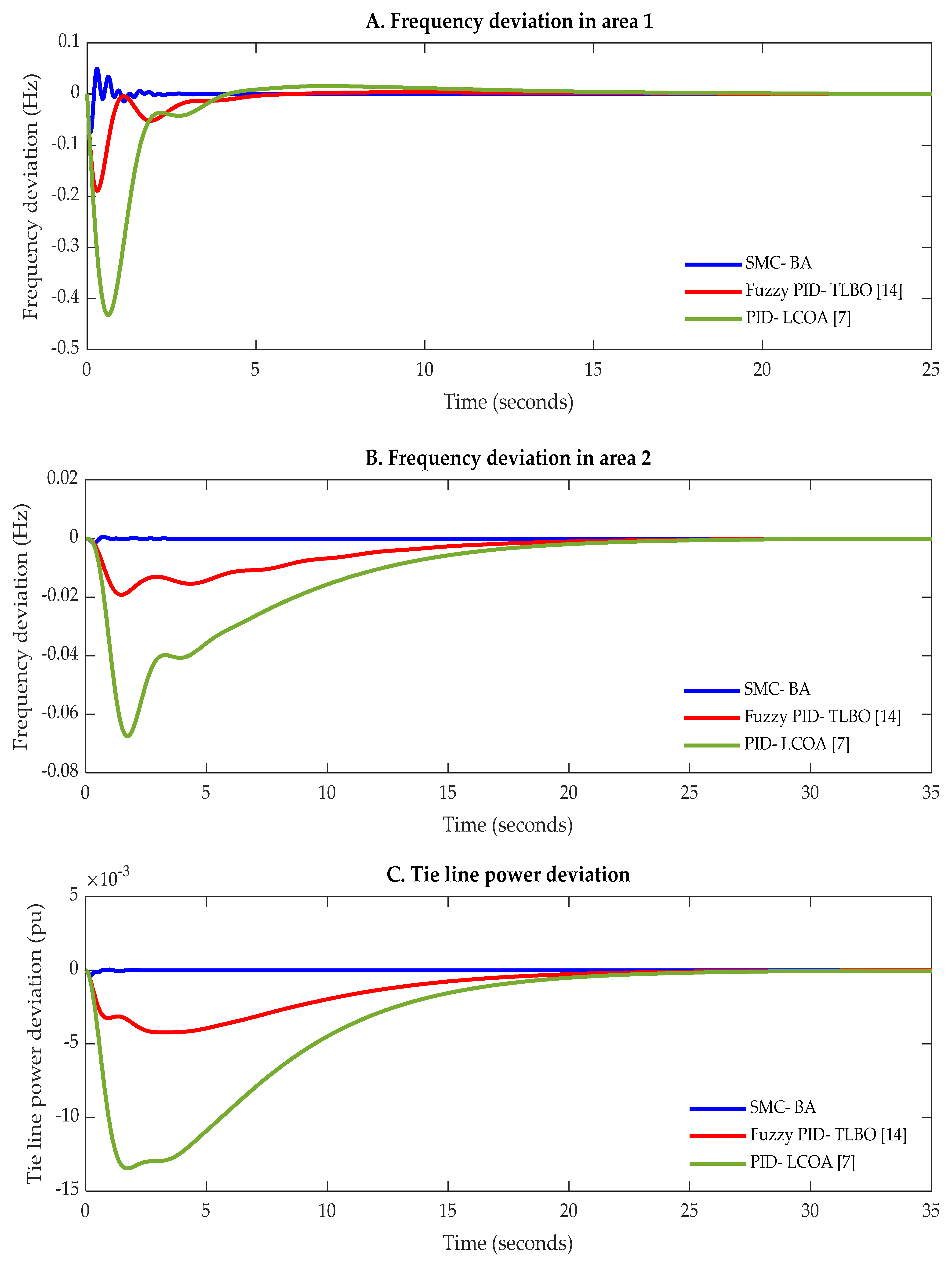
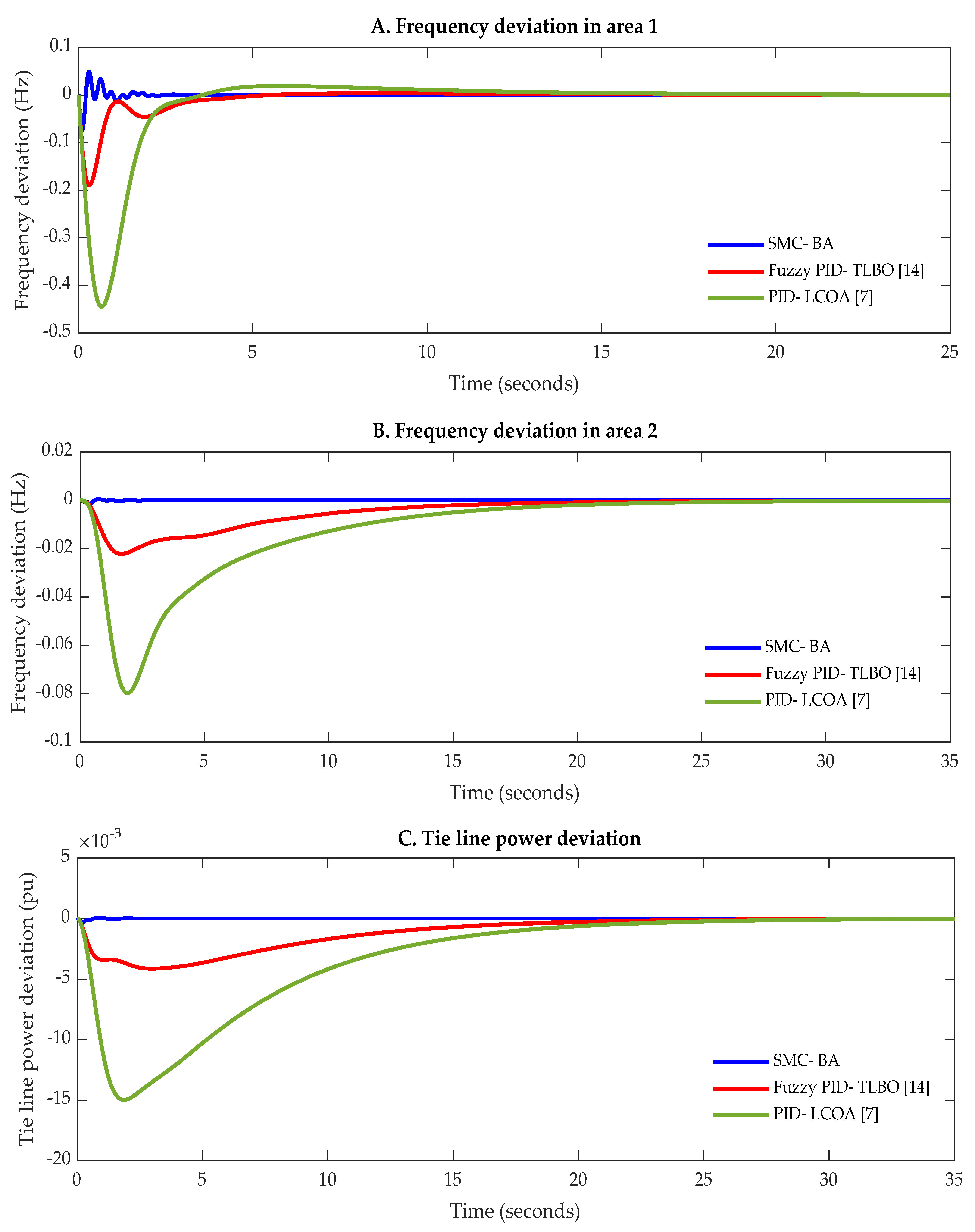
6. Robustness Investigation of SMC

An analysis of the parametric uncertainties in the two-area power system and its impact on the system stability is performed in this section by considering different scenarios. The testbed system has many parameters that may alter during the operating time, alternations in any parameter by increasing or decreasing will influence the overall system stability. For instance, increasing the value of the governor time constant Tg leads to an increase in the frequency fluctuation. While decreasing the damping ratio (D) could increase the frequency deviation which may result in a risk of system instability.

To verify the robustness of the proposed SMC optimised by BA employed in the two-area power model as an LFC system, several scenarios pertaining to the parametric uncertainties of the investigated system are considered as depicted in

Table 6. Different investigated scenarios of system parametric uncertainties.

Case Number	Parameters	Nominal Values		Variation Range	New Values
		Area 1	Area 2		Area 1	Area 2
Case 1	H	5	4	+40%	7	5.6
Case 2	Tt	0.5	0.6	+40%	0.70	0.84
Case 3	B	20.6	16.9	−40%	12.36	10.14
Case 4	D	0.6	0.9	−40%	0.36	0.66
Case 5	Tg	0.2	0.3	+40%	0.28	0.42
Case 6	R	0.05	0.0625	+40%	0.07	0.0875
Case 7	Tg	0.2	0.3	+40%	0.28	0.42
	D	0.6	0.9	−40%	0.36	0.66
Case 8	Tt	0.5	0.6	+40%	0.70	0.84
	B	20.6	16.9	−40%	12.36	10.14
Case 9	Tg	0.2	0.3	+40%	0.28	0.42
	Tt	0.5	0.6	−40%	0.30	0.36
	B	20.6	16.9	−40%	12.36	10.14
Case 10	B	20.6	16.9	−40%	12.36	10.14
	H	5	4	+40%	7	5.6
	R	0.05	0.0625	−40%	0.03	0.0375
	D	0.6	0.9	−40%	0.36	0.66

. Initially, each parameter of the testbed system has been varied individually. Subsequently, several parameters are simultaneously varied by (+ or −) 40% from their nominal values. A step load perturbation of 0.2 pu is applied in area one to observe the impact of the system parametric uncertainties on the performance of the SMC-LFC controller. Similar robustness investigation is carried out for the Fuzzy PID controller optimised by TLBO and the classical PID controller-based LCOA.

In cases 1 to 6 in Table 6, only one parameter is varied at a time. However, in order to make this investigation more realistic, more than one parameter is simultaneously varied from their nominal values. In case 7, the parameters Tg and D in areas one and two are varied by +40% and −40%, respectively. In case 8, the parameters Tt and B in both areas are varied by +40% and −40%, respectively. Furthermore, in case 9, Tg, Tt, and B are varied by +40%, −40% and −40%, respectively. Finally, in case 10, four parameters of the two-area power system are varied from their nominal values, namely, B, H, R and D. These different scenarios could represent the most common conditions of parametric uncertainties that the testbed system may experience in real-time operation.

The frequency variation in area one, frequency variation in area two and tie-line power variation following the implementation of the disturbance in area one under different scenarios of system parametric variations are shown in Figure 7, Figure 8, Figure 9, Figure 10, Figure 11, Figure 12, Figure 13, Figure 14, Figure 15 and Figure 16. In Figure 7, Figure 8, Figure 9, Figure 10, Figure 11, Figure 12, Figure 13, Figure 14, Figure 15 and Figure 16, subfigures (A) illustrate the frequency deviation in area one, subfigures (B) illustrate the frequency deviation in area two and subfigures (C) illustrate the tie line power deviation. Moreover, the dynamic response of the system represented by undershoot $({\mathrm{U}}_{\mathrm{sh}}\mathrm{in} \mathrm{Hz})$, overshoot $({\mathrm{O}}_{\mathrm{sh}}\mathrm{in} \mathrm{Hz})$ and settling time (${\mathrm{T}}_{\mathrm{s}} \mathrm{in} \mathrm{s}$) in $\Delta {\mathrm{F}}_1, \mathrm{and} \Delta {\mathrm{F}}_2$ are presented in

Table 7. Dynamic response of the system under different parametric uncertainties scenarios with different controllers.

Case Number	Controller	Frequency in Area 1			Frequency in Area 2			Tie Line Power Deviation
		${\mathbf{U}}_{\mathbf{sh}}\mathbf{in} \mathbf{Hz}$	${\mathbf{O}}_{\mathbf{sh}}\mathbf{in} \mathbf{Hz}$	${\mathbf{T}}_{\mathbf{s}} \mathbf{in} \mathbf{s}$	${\mathbf{U}}_{\mathbf{sh}}\mathbf{in} \mathbf{Hz}$	${\mathbf{O}}_{\mathbf{sh}}\mathbf{in} \mathbf{Hz}$	${\mathbf{T}}_{\mathbf{s}} \mathbf{in} \mathbf{s}$	${\mathbf{U}}_{\mathbf{sh}}\mathbf{in} \mathbf{pu}$	${\mathbf{O}}_{\mathbf{sh}}\mathbf{in} \mathbf{pu}$	${\mathbf{T}}_{\mathbf{s}} \mathbf{in} \mathbf{s}$
Case 1	SMC-BA	−0.0613	0.0491	2.5551	−0.0014	0.0094	2.3499	−0.0003	0.00008	2.5182
	Fuzzy PID-TLBO	−0.2180	0.0056	12.213	−0.0326	0	23.914	−0.0067	0	24.501
	PID-LCOA	−0.3758	0.0165	12.408	−0.0669	0	21.545	−0.0146	0	22.428
Case 2	SMC-BA	−0.0885	0.0740	2.6330	−0.0022	0.0016	3.1974	−0.0004	0.0001	2.5101
	Fuzzy PID-TLBO	−0.2234	0.0390	4.0000	−0.0252	0	22.329	−0.0042	0	22.469
	PID-LCOA	−0.4917	0.0491	11.007	−0.0863	0	20.3628	−0.0157	0	21.552
Case 3	SMC-BA	−0.0918	0.0840	2.4372	−0.0035	0.0030	3.5679	−0.0004	0.00014	2.3491
	Fuzzy PID-TLBO	−0.3476	0.0057	5.6151	−0.0640	0	26.840	−0.0097	0.00056	34.459
	PID-LCOA	−0.5240	0.0176	10.730	−0.1133	0.0005	17.187	−0.0180	0.00046	20.744
Case 4	SMC-BA	−0.0747	0.0496	2.3248	−0.0016	0.0005	2.4699	−0.0003	0.00005	2.0371
	Fuzzy PID-TLBO	−0.1890	0.0035	4.9709	−0.0192	0	24.814	−0.0042	0	24.933
	PID-LCOA	−0.4319	0.0155	11.743	−0.0675	0	21.596	−0.0135	0	22.753
Case 5	SMC-BA	−0.0874	0.0788	3.6971	−0.0021	0.0014	3.9541	−0.00043	0.00012	3.0577
	Fuzzy PID-TLBO	−0.2146	0.0403	4.6644	−0.0212	0	23.693	−0.0041	0	23.645
	PID-LCOA	−0.4714	0.0165	11.247	−0.0778	0	20.910	−0.0144	0	22.188
Case 6	SMC-BA	−0.0746	0.0492	2.3229	−0.0016	0.0005	2.4716	−0.00032	0.00005	2.0446
	Fuzzy PID-TLBO	−0.1897	0.0036	4.6915	−0.0221	0	23.011	−0.0042	0	26.826
	PID-LCOA	−0.4450	0.0188	11.133	−0.0798	0	20.904	−0.0150	0	23.725
Case 7	SMC-BA	−0.0875	0.0792	3.7032	−0.0021	0.0015	3.9606	−0.00043	0.00012	3.0666
	Fuzzy PID-TLBO	−0.2152	0.0415	4.6671	−0.0215	0	23.395	−0.0042	0	23.753
	PID-LCOA	−0.4750	0.0175	11.183	−0.0793	0	20.832	−0.0145	0	22.242
Case 8	SMC-BA	−0.1087	0.1316	2.5614	−0.0047	0.0059	5.0311	−0.00067	0.00044	2.8036
	Fuzzy PID-TLBO	−0.4015	0.0520	8.5691	−0.0805	0	24.406	−0.0114	0.00056	32.293
	PID-LCOA	−0.5931	0.0730	9.8592	−0.1435	0.0005	16.687	−0.0210	0.00051	20.342
Case 9	SMC-BA	−0.0835	0.0681	2.5323	−0.0029	0.0018	2.28390	−0.00039	0.0001	2.4348
	Fuzzy PID-TLBO	−0.3161	0.0060	10.054	−0.0555	0	28.4522	−0.01030	0.0005	34.399
	PID-LCOA	−0.4820	0.0165	11.008	−0.0975	0.0004	17.5005	−0.01670	0.0004	20.884
Case 10	SMC-BA	−0.0750	0.0872	2.5095	−0.0029	0.0031	4.58160	−0.00045	0.00024	2.4077
	Fuzzy PID-TLBO	−0.3125	0.0060	12.6461	−0.0476	0	39.4405	−0.01090	0.00135	41.302
	PID-LCOA	−0.4094	0.0124	12.4555	−0.0715	0.0010	20.7551	−0.01590	0.00140	27.769

Values that represent the best performance are indicated in bold.

. Additionally, Table 7 provides the undershoot $({\mathrm{U}}_{\mathrm{sh}}\mathrm{in} \mathrm{pu})$, overshoot $({\mathrm{O}}_{\mathrm{sh}}\mathrm{in} \mathrm{pu}),$ and settling time (${\mathrm{T}}_{\mathrm{s}} \mathrm{in} \mathrm{s}$) in $\Delta {\mathrm{P}}_{\mathrm{tie}}$.

Figure 7 shows the dynamic performance of the system based on SMC, Fuzzy PID, and the classical PID under parametric uncertainty case 1, where only the system inertia time constants in both areas are varied by 40% from their nominal values. It is observed that the proposed SMC provided the best performance in terms of undershoot and settling time in the frequency deviation in areas one and two as well as in the tie-line power deviation. Figure 8 indicates the response under parametric uncertainty case 2. In this case, the turbine time constants in both areas are altered by 40%. It is noticed that the increase in the turbine time constant worsened the dynamic response, it caused a further drop in the frequency in both areas. The dynamic response of the system with different controllers under parametric uncertainty case 3 is illustrated in Figure 9. In this case, the nominal values of the frequency bias constants in both areas are varied by −40%. As a result of this variation and based on the results obtained from the SMC tuned by BA, the drop in the frequency in areas one and two have increased from −0.0746 Hz and −0.0016 Hz to −0.0918 Hz and −0.0035 Hz, respectively. In case 4 of robustness analysis towards parametric uncertainty of the testbed system, the value of the coefficient D in both areas are varied by −40%. An extremely slight change in the dynamic performance of the system is observed as shown in Figure 10. However, based on the results obtained for case 5, where the governor time constants in both areas are increased by 40% from their nominal values, a slight increase in the drop in the frequency in both areas is observed as illustrated in Figure 11 and Table 7. In case 6 from the robustness investigation, no obvious change in the dynamic response is observed as shown in Figure 12.

In case 7, the values of Tg and D in both areas are varied by 40% and −40%, respectively. Although two parameters in areas one and two are varied, the proposed SMC-based BA still offering good performance and outperforms the other two controllers as demonstrated in Figure 13. The worst undershoot in the frequency in both areas as well as in the tie-line power deviation is recorded based on the results obtained from case 8 as shown in Figure 14, where the drop of the frequency in area one has increased from −0.0746 Hz to −0.1087 Hz, from −0.1885 Hz to −0.4015 Hz, and from −0.4288 Hz to −0.5931 Hz based on SMC, Fuzzy PID, and classical PID, respectively. Additionally, the drop of the frequency in area two has increased from −0.0016 Hz to −0.0047 Hz, from −0.0190 Hz to −0.0805 Hz, and from −0.0664 Hz to −0.1435 Hz based on SMC, Fuzzy PID, and classical PID, respectively. Whilst the undershoot in the tie-line power has increased from −0.0003 pu to 0.00067 pu, from −0.0042 pu to −0.0114 pu, and from −0.0134 pu to −0.0210 pu based on SMC, Fuzzy PID, and classical PID, respectively. The dynamic response of the system under parametric uncertainty case 9 is demonstrated in Figure 15. In this case of robustness analysis, three different parameters are simultaneously varied. Namely, Tt and B in areas one and two are varied by −40% while the governor time constants Tg are altered by 40%. The notable observed change in the dynamic performance of the system is the slight increase in the drop in the frequency in both areas. Finally, in case 10, four different parameters are varied, the dynamic response of the testbed system under parametric uncertainty case 10 based on SMC, Fuzzy PID and the traditional PID is given in Figure 16.

From Figure 7, Figure 8, Figure 9, Figure 10, Figure 11, Figure 12, Figure 13, Figure 14, Figure 15 and Figure 16 and Table 7, in spite of the wide range of parametric uncertainties of the testbed system in the ten investigated scenarios, the implementation of the proposed SMC design tuned by BA has provided a robust performance which has maintained the system stability within acceptable limits. Furthermore, this controller has outperformed the Fuzzy PID and the traditional PID in terms of the peak undershoot and settling time regardless of the negligible increase in the overshot noted in certain cases.

Moreover, to further assess the performance of the SMC controller, a random load disturbance is applied in area one under the parametric uncertainties of the system case 10 as shown in Figure 17A. The frequency deviation in area one is shown in Figure 17B, the frequency deviation in area two is shown in Figure 17C,D shows the tie line power deviation.

From Figure 17, it is understandable that the proposed SMC-BA controller continues to offer the best dynamic response for frequency variation in area one, frequency variation in area two and tie-line power deviation even with the presence of load disturbance changes every twenty seconds. Additionally, this controller has guaranteed the fastest response with the best-damped oscillation in comparison with Fuzzy PID controller-based TLBO and PID controller tuned by LCOA.

7. Conclusions

In this paper, a novel and simple design of Sliding Mode Control (SMC) is proposed and implemented for Load Frequency Control (LFC) in a dual-area interconnected power system. In order to enhance the performance of the proposed controller, the Bees Algorithm (BA) is proposed in this work as an optimisation tool to find the optimum values of the SMC parameters by minimising integral time absolute error of the frequency variations in both areas and the tie-line power deviation. A step load perturbation of 0.2 pu is applied in area one to study the dynamic behaviour of the testbed system with the proposed decentralised SMC equipped in areas one and two. The superiority of the SMC performance was validated by comparing the results obtained with those of previously published works based on Fuzzy PID and classical PID. Simulation results demonstrated that the SMC tuned by BA performs better than the other reported methods; the peak undershoot and settling time of the frequency deviation in area one has been improved by 82.60% and 80.3055%, respectively, while the same characteristics of the frequency deviation in area two are improved by 97.59% and 88.606%, respectively, as compared with results based on the classical PID tuned by LCOA. Furthermore, the robustness examination of the proposed controller tuned by BA towards a wide range of parametric uncertainties of the investigated system was also performed by considering ten different scenarios. Based on the results obtained from this research, it is revealed that the performance of the proposed SMC design used as LFC in the two-area power system is robust and superior; it provides satisfactory performance in different aspects such as undershoot and settling time regardless of the slight and negligible increase in the overshoot noticed in particular cases. This work can be further extended in future work by implementing the proposed SMC design for LFC in systems that comprise renewable energy resources and considering some nonlinear aspects such as Generation Rate Constraint (GRC) and Governor Deadband (GDB).

References

1. Mohanty, B.; Panda, S.; Hota, P.K. Controller parameters tuning of differential evolution algorithm and its application to load frequency control of multi-source power system. Int. J. Electr. Power Energy Syst. 2014, 54, 77–85. [Google Scholar] [CrossRef]
2. Sahu, B.K.; Pati, T.K.; Nayak, J.R.; Panda, S.; Kar, S.K. A novel hybrid LUS-TLBO optimized fuzzy-PID controller for load frequency control of multi-source power system. Int. J. Electr. Power Energy Syst. 2016, 74, 58–69. [Google Scholar] [CrossRef]
3. Shouran, M.; Anayi, F.; Packianather, M. A State-of-the-Art Review on LFC Strategies in Conventional and Modern Power Systems. In Proceedings of the 2021 International Conference on Advance Computing and Innovative Technologies in Engineering (ICACITE), Greater Noida, India, 4–5 March 2021; pp. 268–277. [Google Scholar]
4. Alhelou, H.H.; Hamedani-Golshan, M.-E.; Zamani, R.; Heydarian-Forushani, E.; Siano, P. Challenges and Opportunities of Load Frequency Control in Conventional, Modern and Future Smart Power Systems: A Comprehensive Review. Energies 2018, 11, 2497. [Google Scholar] [CrossRef] [Green Version]
5. Kozák, S. State-of-the-art in control engineering. J. Electr. Syst. Inf. Technol. 2014, 1, 1–9. [Google Scholar] [CrossRef] [Green Version]
6. Ali, E.S.; Abd-Elazim, S.M. Bacteria foraging optimization algorithm based load frequency controller for interconnected power system. Int. J. Electr. Power Energy Syst. 2011, 33, 633–638. [Google Scholar] [CrossRef]
7. Farahani, M.; Ganjefar, S.; Alizadeh, M. PID controller adjustment using chaotic optimisation algorithm for multi-area load frequency control. IET Control Theory Appl. 2012, 6, 1984–1992. [Google Scholar] [CrossRef]
8. Zamani, A.; Barakati, S.M.; Yousofi-Darmian, S. Design of a fractional order PID controller using GBMO algorithm for load–frequency control with governor saturation consideration. ISA Trans. 2016, 64, 56–66. [Google Scholar] [CrossRef]
9. Çelik, E. Design of new fractional order PI–fractional order PD cascade controller through dragonfly search algorithm for advanced load frequency control of power systems. Soft Comput. 2021, 25, 1193–1217. [Google Scholar] [CrossRef]
10. Ersdal, A.M.; Fabozzi, D.; Imsland, L.; Thornhill, N.F. Model predictive control for power system frequency control taking into account imbalance uncertainty. IFAC Proc. Vol. 2014, 47, 981–986. [Google Scholar] [CrossRef] [Green Version]
11. Badihi, H.; Zhang, Y.; Hong, H. Design of a pole placement active power control system for supporting grid frequency regulation and fault tolerance in wind farms. IFAC Proc. Vol. 2014, 47, 4328–4333. [Google Scholar] [CrossRef] [Green Version]
12. Davidson, R.A.; Ushakumari, S. H-infinity loop-shaping controller for load frequency control of a deregulated power system. Procedia Technol. 2016, 25, 775–784. [Google Scholar] [CrossRef] [Green Version]
13. Kasireddy, I.; Nasir, A.W.; Singh, A.K. IMC based Controller Design for Automatic Generation Control of Multi Area Power System via Simplified Decoupling. Int. J. Control Autom. Syst. 2018, 16, 994–1010. [Google Scholar] [CrossRef]
14. Sahu, B.K.; Pati, S.; Mohanty, P.K.; Panda, S. Teaching-learning based optimization algorithm based fuzzy-PID controller for automatic generation control of multi-area power system. Appl. Soft Comput. J. 2015, 27, 240–249. [Google Scholar] [CrossRef]
15. Shouran, M.; Anayi, F.; Packianather, M.; Habil, M. Load Frequency Control Based on the Bees Algorithm for the Great Britain Power System. Designs 2021, 5, 50. [Google Scholar] [CrossRef]
16. Huang, C.-I.; Lian, K.-Y.; Chiu, C.-S.; Fu, L.-C. Smooth Sliding Mode Control for Constrained Manipulator with Joint Flexibility. IFAC Proc. Vol. 2005, 38, 91–96. [Google Scholar] [CrossRef] [Green Version]
17. Wang, Y.; Sun, L. On the Optimized Continuous Nonsingular Terminal Sliding Mode Control of Flexible Manipulators. In Proceedings of the 2014 Fourth International Conference on Instrumentation and Measurement, Computer, Communication and Control, Harbin, China, 18–20 September 2014; pp. 324–329. [Google Scholar] [CrossRef]
18. Chen, H.-Y.; Huang, S.-J. Adaptive fuzzy sliding-mode control for the Ti6Al4V laser alloying process. Int. J. Adv. Manuf. Technol. 2004, 24, 667–674. [Google Scholar] [CrossRef]
19. Patre, B.M.; Londhe, P.S.; Nagarale, R.M. Fuzzy Sliding Mode Control for Spatial Control of Large Nuclear Reactor. IEEE Trans. Nucl. Sci. 2015, 62, 2255–2265. [Google Scholar] [CrossRef]
20. Nair, R.R.; Behera, L. Robust adaptive gain nonsingular fast terminal sliding mode control for spacecraft formation flying. In Proceedings of the 2015 54th IEEE Conference on Decision and Control (CDC), Osaka, Japan, 15–18 December 2015; pp. 5314–5319. [Google Scholar] [CrossRef]
21. Xu, S.S.-D.; Chen, C.-C.; Wu, Z.-L. Study of Nonsingular Fast Terminal Sliding-Mode Fault-Tolerant Control. IEEE Trans. Ind. Electron. 2015, 62, 3906–3913. [Google Scholar] [CrossRef]
22. Hemke, G.D.; Daingade, S. Fast Terminal Sliding Mode based DC-DC Buck converter. In Proceedings of the 2016 IEEE 1st International Conference on Power Electronics, Intelligent Control and Energy Systems (ICPEICES), Delhi, India, 4–6 July 2016; pp. 1–4. [Google Scholar] [CrossRef]
23. Defoort, M.; Nollet, F.; Floquet, T.; Perruquetti, W. A Third-Order Sliding-Mode Controller for a Stepper Motor. IEEE Trans. Ind. Electron. 2009, 56, 3337–3346. [Google Scholar] [CrossRef]
24. Mi, Y.; Fu, Y.; Li, D.; Wang, C.; Loh, P.C.; Wang, P. The sliding mode load frequency control for hybrid power system based on disturbance observer. Int. J. Electr. Power Energy Syst. 2016, 74, 446–452. [Google Scholar] [CrossRef]
25. Vrdoljak, K.; Perić, N.; Petrović, I. Sliding mode based load-frequency control in power systems. Electr. Power Syst. Res. 2010, 80, 514–527. [Google Scholar] [CrossRef]
26. Kumar, A.; Anwar, M.N.; Kumar, S. Sliding mode controller design for frequency regulation in an interconnected power system. Prot. Control Mod. Power Syst. 2021, 6, 6. [Google Scholar] [CrossRef]
27. Guo, J. Application of full order sliding mode control based on different areas power system with load frequency control. ISA Trans. 2019, 92, 23–34. [Google Scholar] [CrossRef]
28. Mohanty, B. TLBO optimized sliding mode controller for multi-area multi-source nonlinear interconnected AGC system. Int. J. Electr. Power Energy Syst. 2015, 73, 872–881. [Google Scholar] [CrossRef]
29. Huynh, V.V.; Tran, P.T.; Minh, B.L.N.; Tran, A.T.; Tuan, D.H.; Nguyen, T.M.; Vu, P.-T. New Second-Order Sliding Mode Control Design for Load Frequency Control of a Power System. Energies 2020, 13, 6509. [Google Scholar] [CrossRef]
30. Huynh, V.V.; Minh, B.L.N.; Amaefule, E.N.; Tran, A.-T.; Tran, P.T. Highly Robust Observer Sliding Mode Based Frequency Control for Multi Area Power Systems with Renewable Power Plants. Electronics 2021, 10, 274. [Google Scholar] [CrossRef]
31. Tran, A.-T.; Minh, B.L.N.; Huynh, V.V.; Tran, P.T.; Amaefule, E.N.; Phan, V.-D.; Nguyen, T.M. Load Frequency Regulator in Interconnected Power System Using Second-Order Sliding Mode Control Combined with State Estimator. Energies 2021, 14, 863. [Google Scholar] [CrossRef]
32. Pham, D.T.; Ghanbarzadeh, A.; Koç, E.; Otri, S.; Rahim, S.; Zaidi, M. The Bees Algorithm—A Novel Tool for Complex Optimisation Problems. In Intelligent Production Machines and Systems; Elsevier: Amsterdam, The Netherlands, 2006; pp. 454–459. [Google Scholar]
33. Pham, D.T.; Castellani, M. A comparative study of the Bees Algorithm as a tool for function optimisation. Cogent Eng. 2015, 2, 1091540. [Google Scholar] [CrossRef]
34. Fahmy, A.A. Using the Bees Algorithm to select the optimal speed parameters for wind turbine generators. J. King Saud Univ. -Comput. Inf. Sci. 2012, 24, 17–26. [Google Scholar] [CrossRef] [Green Version]
35. Packianather, M.S.; Al-Musawi, A.K.; Anayi, F. Bee for mining (B4M)—A novel rule discovery method using the Bees algorithm with quality-weight and coverage-weight. Proc. Inst. Mech. Eng. Part C J. Mech. Eng. Sci. 2019, 233, 5101–5112. [Google Scholar] [CrossRef]
36. Zhou, Z.; Xie, Y.; Pham, D.; Kamsani, S.; Castellani, M. Bees Algorithm for multimodal function optimisation. Proc. Inst. Mech. Eng. Part C J. Mech. Eng. Sci. 2016, 230, 867–884. [Google Scholar] [CrossRef]
37. Chamazi, M.A.; Motameni, H. Finding suitable membership functions for fuzzy temporal mining problems using fuzzy temporal bees method. Soft Comput. 2019, 23, 3501–3518. [Google Scholar] [CrossRef]
38. Pham, D.T.; Kalyoncu, M. Optimisation of a fuzzy logic controller for a flexible single-link robot arm using the bees algorithm. In Proceedings of the IEEE International Conference on Industrial Informatics (INDIN), Cardiff, UK, 23–26 June 2009; pp. 475–480. [Google Scholar]
Figure 1. Transfer function model of the testbed system.
Energies 14 05701 g001
Figure 2. The Bees Algorithm flowchart.
Energies 14 05701 g002
Figure 3. Frequency deviation in area one ( Δ F 1 in Hz).
Energies 14 05701 g003
Figure 4. Frequency deviation in area two ( Δ F 2 in Hz).
Energies 14 05701 g004
Figure 5. Tie line power deviation ( Δ P tie in pu).
Energies 14 05701 g005
Figure 6. Percentage of improvement in undershoot, settling time and ITAE with different controllers.
Energies 14 05701 g006
Figure 7. Dynamic response of the system with different controllers under parametric uncertainties, case 1. (A) Frequency deviation in area 1; (B) Frequency deviation in area 2; (C) Tie line power deviation.
Energies 14 05701 g007
Figure 8. Dynamic response of the system with different controllers under parametric uncertainties, case 2. (A) Frequency deviation in area 1; (B) Frequency deviation in area 2; (C) Tie line power deviation.
Energies 14 05701 g008
Figure 9. Dynamic response of the system with different controllers under parametric uncertainties, case 3. (A) Frequency deviation in area 1; (B) Frequency deviation in area 2; (C) Tie line power deviation.
Energies 14 05701 g009
Figure 10. Dynamic response of the system with different controllers under parametric uncertainties, case 4. (A) Frequency deviation in area 1; (B) Frequency deviation in area 2; (C) Tie line power deviation.
Energies 14 05701 g010
Figure 11. Dynamic response of the system with different controllers under parametric uncertainties, case 5. (A) Frequency deviation in area 1; (B) Frequency deviation in area 2; (C) Tie line power deviation.
Energies 14 05701 g011
Figure 12. Dynamic response of the system with different controllers under parametric uncertainties, case 6. (A) Frequency deviation in area 1; (B) Frequency deviation in area 2; (C) Tie line power deviation.
Energies 14 05701 g012
Figure 13. Dynamic response of the system with different controllers under parametric uncertainties, case 7. (A) Frequency deviation in area 1; (B) Frequency deviation in area 2; (C) Tie line power deviation.
Energies 14 05701 g013
Figure 14. Dynamic response of the system with different controllers under parametric uncertainties, case 8. (A) Frequency deviation in area 1; (B) Frequency deviation in area 2; (C) Tie line power deviation.
Energies 14 05701 g014
Figure 15. Dynamic response of the system with different controllers under parametric uncertainties, case 9. (A) Frequency deviation in area 1; (B) Frequency deviation in area 2; (C) Tie line power deviation.
Energies 14 05701 g015
Figure 16. Dynamic response of the system with different controllers under parametric uncertainties, case 10. (A) Frequency deviation in area 1; (B) Frequency deviation in area 2; (C) Tie line power deviation.
Energies 14 05701 g016
Figure 17. Dynamic response of the system with different controllers under parametric uncertainties, case 10 with a random load disturbance applied in area one. (A) Random load disturbance; (B) Frequency deviation in area 1; (C) Frequency deviation in area 2; (D) Tie line power deviation.
Energies 14 05701 g017