Article

An Ultra-Fast Power Prediction Method Based on Simplified LSSVM Hyperparameters Optimization for PV Power Smoothing

1
School of Electrical and Information Engineering, Hunan Institute of Engineering, Xiangtan 411100, China
2
Growatt New Energy Technology (Thailand) Co., Ltd., Shenzhen 518000, China
3
School of Electrical and Electronic Engineering, Wenzhou University, Wenzhou 325000, China
*
Author to whom correspondence should be addressed.
Energies 2021, 14(18), 5752; https://doi.org/10.3390/en14185752
Submission received: 10 August 2021 / Revised: 25 August 2021 / Accepted: 3 September 2021 / Published: 13 September 2021
(This article belongs to the Special Issue Frontier in Special Power Conversion Systems and Control)

Abstract

:
With existing power prediction algorithms, it is difficult to satisfy the requirements for prediction accuracy and time when PV output power fluctuates sharply within seconds, so this paper proposes a high-precision and ultra-fast PV power prediction algorithm. Firstly, in order to shorten the optimization time and improve the optimization accuracy, the single-iteration Gray Wolf Optimization (SiGWO) method is used to simplify the iteration process of the hyperparameters of Least Squares Support Vector Machine (LSSVM), and then the hybrid local search algorithm composed of Iterative Local Search (ILS) and Self-adaptive Differential Evolution (SaDE) is used to improve the accuracy of hyperparameters, so as to achieve high-precision and ultra-fast PV power prediction. The power prediction model is established, and the proposed algorithm is applied in a test experiment which can complete the power prediction within 3 s, and the RMSE is only 0.44%. Finally, combined with the PV-storage advanced smoothing control strategy, it is verified that the performance of the proposed algorithm can satisfy the system’s requirements for prediction accuracy and time under the condition of power mutation in a PV power generation system.

1. Introduction

In recent years, the penetration rate of renewable energy such as solar energy has increased [1]. PV power generation is easily affected by the environment, resulting in power fluctuations lasting for several seconds to several minutes [2], in which the maximum instantaneous power fluctuation rate can reach 75%/s [3], causing grid voltage and frequency flicker, which will reduce power quality and power supply reliability [4,5].
It has been proven that the PV power station equipped with energy storage can smooth the power fluctuation effectively [6,7]; especially, the energy storage system with high power density can effectively smooth the short-term and severe PV power fluctuation [8]. In Guo T., Liu Y., Zhao J. et al. [9], a new robust dynamic wavelet-enabled method is proposed, which can optimize the wavelet parameters adaptively and adjust the state of charge (SOC) and depth of charge or discharge of the hybrid energy storage system (HESS) composed of supercapacitors and batteries so as to smooth the fluctuations of the output power. In Sun Y., Tang X., Sun X., et al. [10], an improved low-pass filtering algorithm (ILFA) is proposed to optimize the power distribution of the battery and the supercapacitor, and it combines with the fuzzy control (FC) to smooth the power fluctuations based on the SC priority control strategy. In Lamsal, D., Sreeram, V., et al. [7], a fuzzy-based discrete Kalman filter method is proposed to adaptively adjust the battery power by using the battery SOC as the feedback of energy storage to stabilize the output power fluctuations. There is no energy storage medium with the outstanding characteristics and comprehensive ability [11]; therefore, the above methods choose the HESS with complementary advantages [6]. However, considering the real-time nature of the HESS operation control [12] and the high uncertainty of the future output power [13], the above methods are difficult to adapt to the high complexity of the future output power, the real-time optimization control of the energy storage systems.
The energy storage smoothing method based on the power prediction can optimize the configuration of the energy storage in advance, and reduce the uncertainty of the future output power, and optimize energy storage control [14,15,16,17,18]. In Zhang Xinsong et al. [14], a wind-storage hybrid power station with a dual-battery energy storage system topology is proposed. The predicted power is obtained by the average movement method, and the power fluctuations is stabilized under the guidance of the predicted power. This method can effectively smooth the power fluctuations in the next 15 min, but the RSD is up to 2.5%, which will affect the power prediction results when the output power fluctuates slightly. In Qian W. et al. [15], the probability prediction is used to obtain the predicted power, and the predicted power is decomposed with HESS, so as to determine the scheduled grid-connected power and smooth the power fluctuations. However, its power deviation is up to 8.4%, which reduces the requirement of prediction accuracy and leads to the reduction in prediction power under the reference. In Wang Y., Tai N., Huang W., et al. [16], a rolling coordinated control scheme of hybrid power system based on the ultra-short-term power prediction is proposed. Firstly, the predicted power is obtained based on forward neural network algorithm (BPNN), and the filter coefficient (FC) is optimized by PSO algorithm. Finally, the low-pass filtering and SOC are combined to smooth the output power fluctuations, but after data acquisition and calculation, its RMSE is up to 4.73%, and the accuracy of power smoothing is reduced. In Islam F. et al. [17], a wind speed prediction model based on radial basis function neural network (RBFNN) is established to minimize the output power fluctuations with the combination of the supervisory control unit (SCU). However, the power prediction is indirectly obtained by the wind speed prediction, and after data acquisition and calculation, its RMSE is up to 13.5%. In Pan Yifu, Yang Junhua [18], the extreme learning machine was used to predict the output power of wave generation, and combined with hybrid energy storage, the charge and discharge of the energy storage system are controlled according to the predicted power to realize the power smoothing of the wave electric system. However, the RMSE of power prediction is up to 3.8%. References [14,15,16,17,18] smooth the power fluctuations within a short period based on power prediction, but the accuracy of such methods is on the low side. The existing ultra-short-term and high-precision power prediction is mostly used in power dispatching applications with a sampling interval of 15 min [19], and the time required for power prediction is mostly 5–10 min, which can effectively meet the requirements of power system dispatching. However, faced with the problem that the PV power fluctuates violently in a few seconds like in reference [3], the existing power prediction algorithm has a long prediction time, resulting in a large sampling interval, so it is difficult to perceive the power fluctuation in a few seconds or tens of seconds. Therefore, a new method is needed to complete high-precision power prediction in a few seconds.
Regarding the issue above, a high-precision and ultra-fast PV power prediction algorithm recorded as HLSGWO-LSSVM is proposed. Applying the proposed algorithm to practice, which can complete the power prediction within 3 s, and the RMSE is only 0.44%,the superiority of the proposed algorithm can be stressed.
The content of paper includes an introduction to the principle of the proposed algorithm in Section 2, a comparison of the proposed algorithm with existing algorithms in Section 3, the application of the proposed algorithm to smooth the power fluctuations of the PV power generation system in Section 4, and the conclusion of this paper in Section 5.

2. The Principle of the Proposed Algorithm

2.1. LSSVM Algorithm and Hyperparameters

Compared with the wavelet analysis and neural networks, support vector machine (SVM) has obvious advantages in self-learning, self-adaptation, and non-linear mapping, but its training speed for quadratic programming problems is slow. The least square support vector machine (LSSVM) on the basis of SVM is proposed by Suykens [20], which chooses the principle of minimizing structural risk, and converts the optimization problem into a form similar to ridge regression. The difficulty of solving to a certain extent is reduced and the solution speed is improved. According to the principle of structural risk minimization, the regression problem is transformed into an equation-constrained optimization problem:
min β , e   g ( β , e ) = 1 2 β T β + C 2 i = 1 n e i 2 i = 1 , 2 , n s . t . y i [ β T φ ( x i ) + b ] = 1 e i
where ei is the error variate, βT is the hyperplane normal vector in high-dimensional space, b is the offset, φ ( x ) is the non-linear mapping function, and C is the regular parameter which used to balance the complexity of the model.
The model of LSSVM is as follows:
y ( x ) = i = 1 N α i K ( x , x i ) + b
where αi is the Lagrange multipliers and K(x, xi) is the kernel function.
This paper selects the RBF kernel as the kernel function, defined as the monotonic function of the Euclidean distance from any point x to a certain center xc in space [21].
The kernel function K(x, xi) is as follows:
K ( x , x c ) = exp ( | | x x c | | 2 σ 2 )
where x is the any point in space, xc is the center point in space, and σ is the width parameter of the kernel function.
The regression of LSSVM is related to the choice of hyperparameters which are included with the regular parameter C and the width parameter σ of the kernel function [22].

2.2. Hyperparameters Optimization for the First Time

Mirjalili imitates the hunting process of the gray wolf and proposes the Gray Wolf Optimization (GWO) [23]. Under the guidance of the optimization ideology of GWO, this paper proposes a Single-iteration Gray Wolf Optimization (SiGWO) to optimize hyperparameters for the first time. In the GWO algorithm, the process of iteration is the process of wolf α, wolf β, and wolf δ constantly approaching their prey. The distance Dα, Dβ, and Dδ between wolves ω and wolf α, wolf β, and wolf δ is continuously shortened by the iterative calculation to narrow the encircling radius, and the optimal hyperparameters are obtained.
The schematic diagram of the hunting process of the gray wolves is shown in Figure 1.
According to the single iteration principle of the SiGWO, the gray wolves only hunt for the prey (the optimal solution) once, and narrow the hunting radius to the range by r shown in Figure 1. The approximate position of the prey (the optimal solution) is defined and recorded as the position solution Xpos. The above process is recorded as the first optimization of the hyperparameters.

2.3. Chaos Initialization

Chaos is a widespread phenomenon in nonlinear systems, and chaotic mapping instead of traditional probability distribution is used to initialize the population which can enhance the traversal and uniformity of the population [24]. The cube map which has better uniformity is chosen to complete the initialization of the gray wolf. The formula for cube mapping is as follows:
{ y ( n + 1 ) = 4 y 3 ( n ) 3 y ( n ) 1 y ( n ) 1 , n = 0 , 1 , 2 ,
where y(n) is the chaos number generated by chaos initialization and n is the size of the gray wolf population.
Chaos is a complex system with unpredictable behavior, and mapping is to associate chaotic behavior with a parameter by a function [24]. The original pseudo-random numbers are replaced by chaotic numbers in the proposed algorithm, and the position is calculated.
P o s i t i o n = ( 1 + y ( n ) ) ( u b l b 2 ) + l b
where Position is the initialization position and ub and lb are the upper and lower bounds of the parameter value, respectively.
This paper sums up the detailed introduction of the SiGWO algorithm and chaos initialization above, and records the specific process of the algorithm in the form of pseudo code, as shown in Figure 2.

2.4. Hyperparameters Accuracy Optimized by Hybrid Local Search

A hybrid local search is introduced to improve the accuracy of the hyperparameters, and the Xpos, which has experienced chaos initialization, will be used as the initial solution for the hybrid local search.
(1) Preliminary optimization of accuracy. Iterative local search (ILS) is based on the common characteristics of good solutions, adding local disturbance to the existing position solution Xpos [25], using the Griewank function as a perturbation function [26], disturbing the existing solution to ensure that it jumps out of the local optimum to find the new position solution betterpos.
The formula of the Griewank function is as follows:
x i = X pos r a n d n G = 1 + 1 4000 i = 1 n x i 2 i = 1 n cos ( x i i )
where Xpos is the position solution obtained by the SiGWO algorithm, randn is the stochastic number between [−1, 1], xi is the stochastic product of Xpos, and G is the disturbance output.
(2) Re-optimization of accuracy. In order to find the optimal hyperparameters, a Self-adaptive Differential Evolution Algorithm (SaDE) is introduced. The second local search is used to confirm the position information of the wolf α in the optimal population to obtain the optimal hyperparameters. The global or local search ability of the algorithm will be affected by the definition of the variation factor F [27]. Therefore, the variation factor F of the SaDE algorithm is defined as follows:
F = F 0 2 exp ( 1 M a x _ i t e r a t i o n s M a x _ i t e r a t i o n s + 1 i )
where F0 is the initial variation factor, i is the ith population, and Max_iteration is the maximum number of iterations.
The mutation strategy of SaDE algorithm is as follows:
d d = 2 2 × M a x _ i t e r a t i o n s + 1 i M a x _ i t e r a t i o n s b e s t pos = d d b e t t e r pos + F ( N i 2 ( t ) N i 3 ( t ) )
where dd is the adaptive parameter, betterpos is the better solution of position, Ni2(t) and Ni3(t) is the random vector, and bestpos is the position of the optimal solution.
Based on the content above, the pseudo code of the hybrid local search algorithm is shown in Figure 3.
Under the guidance of the principle of one-to-one correspondence between the population fitness and the position, the optimal position is determined by the search of the minimum population fitness. The information of the optimal hyperparameters is contained in the optimal position.
The main flow chart of the proposed algorithm is shown in Figure 4.

3. Comparison between the Proposed Algorithm and the Existing Algorithm

3.1. Data Collection

The existing power prediction methods are based on solar radiation intensity, historical power, and meteorological factors to complete the power prediction by statistical prediction or intelligent algorithm. However, these methods cannot adequately study the power fluctuation characteristics, and the accuracy of the prediction is impacted by over-reliance on Numerical Weather Prediction (NWP), which is low-precision and high-cost [28].
This paper divides the historical output power into every 1 min in PV power station in Shenzhen. It updates the sampling power based on the cyclic forecasting idea, adds the latest measured data, and eliminates the furthest measured data. The basic weather conditions of the selected sample data are as follows: the temperature at the time of sample collection is 24–27 ℃, cloudy, and northeast wind level 3.

3.2. Data Classification and Normalization

This paper selects the six-hour historical output power of the PV power as a sample, the last half-hour output power as the test data, and the rest as the training data.
The speed of convergence and the accuracy will be improved because the sample data are normalized. The min-max standardization method is selected to linearly transform the original data, so that the result value x* is mapped to [0, 1].
The conversion function is as follows:
x * = x x min x max x min
where xmax and xmin are the maximum and minimum values in the sample data, respectively, and x* is the normalized value.

3.3. Predictive Evaluation Index

A simulation is built to record the prediction time and the accuracy of the predicted power at the same time. The mean absolute percentage error (MAPE) and root mean square error (RMSE) are used to evaluate the accuracy of the predicted power.
M A P E = 100 % N i = 1 N | y i y ^ i y i |
R M S E = 1 N i = 1 N ( y i y ^ i ) 2
where N is the number of training or test samples, yi is the actual value, and y ^ i is the predicted value.

3.4. Simulation Verification

Several existing high-precision power prediction algorithms such as QPSO-LSSVM, SaDE-GWO-LSSVM, and ABC-LSSVM are chosen as the control group, compared with the proposed algorithm, and run under the same sample data. MATLAB is used to simulate the above algorithm, and the prediction algorithm is evaluated from the two aspects of prediction accuracy and time.
In order to reduce the effect of prediction randomness, the average power after 20 times of prediction in the same period is selected as the final prediction power.
The fitting curve of the predicted power obtained by the power prediction algorithms and the actual power is shown in Figure 5.
As shown in Figure 5, the degree of fitting between the predicted power and the actual power is at a high level, and the degree of fitting of the power curve is positively correlated with the accuracy. By comparing the deviation degree of each predicted power, we can gain the following prediction accuracy results: QPSO-LSSVM > HLSGWO-LSSVM > ABC-LSSVM > SaDE-GWO-LSSVM.
According to the definition of the power prediction evaluation index, this paper selects the RMSE to draw the prediction. To sum up the above, the chart of error–time comparison is shown in Figure 6.
As can be seen from Figure 6, the proposed algorithm can complete the power prediction within 3 s and greatly shorten the time required for power prediction. In this case, the sampling interval could be further shortened, and the sensitivity of the smoothing system to the power fluctuations in an ultra-short period can be enhanced.
Understanding the occupancy of the power prediction in PV power generation systems is of great significance to the internal resource allocation of PV power generation systems. The paper uses AIDA64 software to monitor the computer CPU occupancy rate of each power prediction algorithm when it works. A histogram is used to represent the total occupancy rate of each power prediction algorithm in the PV power generation system, as shown in Figure 7.
The total occupancy rate of the prediction algorithm is the sum of the system occupancy rate in each time period when the prediction algorithm is running. The higher its value, the higher the performance requirements of the CPU, and the high total occupancy rate will affect the operation of other parts in the PV power generation system.
As shown in Figure 7, the proposed algorithm can greatly reduce the resource occupancy rate for the power prediction calculation in the PV power generation system, and then relieve the pressure of computer calculation and improve the operating efficiency of the power generation systems.

3.5. Comprehensive Analysis of Predictive Power

The RMSE, which is sensitive to the abnormal values, is selected as the main evaluation index of the prediction error, and the RMSE between the predicted power and the actual power is calculated every minute in the future. The distribution diagram of the prediction error (RMSE) at each time point of power prediction is shown in Figure 8.
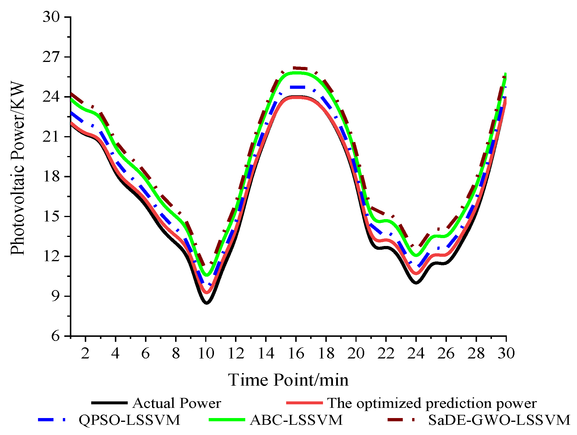
As shown in Figure 8, by analyzing the RMSE index of each power prediction value, the prediction error RMSE curve of the proposed algorithm changes most gently. By comparing Figure 5 and Figure 8, the power prediction curve of the proposed algorithm can be regarded as the translation of the actual power curve.
In order to verify the universality of this discovery, it needs to be verified later. After verification, it is found that the power prediction curve of the same PV power station at different times or under different weather conditions can show a high fit with the actual power curve after translation change, and the translation range is relatively stable and fluctuates in a small range.
Therefore, the above predicted power can be translated and calculated, and the fitting diagram of the translated power prediction curve can be drawn in Figure 9.
The new power prediction fitting curve after translation and calculation is shown in Table 1.
According to the comprehensive analysis of Table 1 and Figure 9, the proposed algorithm has the best fit between the predicted power curve and the actual power curve, which greatly improves the accuracy of power prediction.

4. Power Smoothing Application of the Proposed Algorithm

4.1. PV Power Generation System Equipped with HESS

HESS, which is composed of energy storage batteries and supercapacitors, is selected to complete the power smoothing. HESS combines the advantages of both, which has high energy density and power density at the same time and ensures the energy storage can smooth the power fluctuation efficiently and quickly.
The schematic diagram of the PV power generation system equipped with HESS is shown in Figure 10.
All parts in Figure 10 obey the law of conservation of energy that can be summarized as the following formula:
P pv + P HESS = P Grid
where Ppv is the output power of PV, PHESS is the charge or discharge power of HESS, and PGrid is the grid-connected power.

4.2. Related Parameter Settings

It is assumed that the energy storage system in this paper is an ideal energy storage, meaning that the capacity is sufficient to satisfy the requirements for power smoothing.
(1) Sampling interval T0. The PV power generation is a continuous process; as long as the power generation conditions are met, electric energy can be generated in real time. It is assumed that the power of PV power generation during T0 is a constant value.
(2) Power fluctuation rate ΔP′. The ratio of the output power difference between adjacent power sampling points to time. The calculation formula is:
Δ P ( t ) = P ( t ) P ( t 1 ) Δ P ( t ) = Δ P ( t ) T 0 t = 1 , 2 , , n
where t is the tth sampling point after the prediction time, P(t) is the predicted power at time t, and ΔP′(t) is the power fluctuation rate at time t.
(3) Target volatility Det. Det is a parameter that can reflect the power grid’s frequency modulation capability; it is the upper bound of the grid-connected power fluctuation allowed in the guidelines [29]. The grid-connected PV power needs to satisfy the following formula:
| P ( t ) P ( t 1 ) | D et

4.3. The Design of PV-Storage Advanced Smoothing Control Strategy

The charge or discharge action of HESS is judged by the fluctuation rate between the prediction power and target volatility Det. When the predicted power fluctuation rate is greater than Det, HESS will charge or discharge; otherwise, there is no action [30].
The specific control strategy is as follows:
P HESS ( t ) = { 0 | Δ P ( t ) | < D et Δ P ( t ) D et Δ P ( t ) > D et Δ P ( t ) + D et Δ P ( t ) < D et
where PHESS(t) is the charge or discharge power of HESS at time t.
The energy exchange can be completed in advance according to the predicted power, so as to ensure the energy storage system can satisfy the charge or discharge.
The flow chart of PV-storage advanced smooth control is shown in Figure 11.

4.4. The Verification of Power Smoothing Simulation

The predicted power is gained by the power prediction algorithm. HESS follows the flow of advanced smoothing control strategy to realize charge or discharge, in order to compensate the difference between the predicted power and the grid-connected target value.
In addition, according to China’s State Grid Enterprise Standard Q/GDW617-2011 “Technical Regulations for Connecting Photovoltaic Power Stations to the Grid”, the maximum active power change of a small PV power station within 1 min is limited to 0.2 MW. Therefore, this paper sets the target volatility Det to 2 KW/min.
A schematic diagram of power smoothing based on predicted power is shown in Figure 12.
As shown in Figure 12, the power smoothing based on the predicted power can effectively solve the problem of the sharp fluctuations within seconds. In combination Figure 8 with Table 1, the relationship between the power smoothing performance and the power prediction accuracy shows that the storage power smoothing performs well when it under the guidance of the predicted power with high-precision. The slight power fluctuation such as at the 14th sampling time point can be smoothed well by HESS, and the smoothness of the grid-connected power can be improved, in order to guarantee the power quality of the whole power system.
The charge or discharge power of HESS is shown in Figure 13.
As can be seen from the Figure 12 and Figure 13, the grid-connected power under the guidance of high-precision power prediction has a higher degree of fit with the actual power.
The power required for power smoothing for a single time is reduced by 4.5% to 5%. At the same time, the power smoothing guided by the proposed algorithm reduces the capacity requirements of energy storage equipment.

5. Conclusions

This paper proposes a high-precision and ultra-fast PV power prediction algorithm, in view of the difficulty of the existing power prediction algorithms to simultaneously satisfy the requirements for prediction accuracy and time when the PV output power fluctuates sharply within seconds.
By comparison with the existing power prediction algorithms, the proposed algorithm can complete power prediction within 3 s and greatly reduce the time required for power prediction. According to the predicted power error distribution, the RMSE of the proposed algorithm optimized is only 0.44%.
The proposed algorithm is applied to the PV-storage advanced smoothing control to prove that this algorithm can effectively guide the smoothing of HESS, and ensures the smoothness of the grid-connected power. In addition, the proposed algorithm can reduce the requirements of the energy storage capacity to a certain degree.

6. Patents

Zhenxing Zhao, Kaijie Chen, Yuxing Dai, Ying Chen, Daopu Xiang, Kuiyin Zhao, Yong Ning, Zeng Liu, Huan Wang. A second level ultra short term photovoltaic power prediction method [P]. Hunan Province: cn112507613a, 2021-03-16.

Author Contributions

Conceptualization, Z.Z.; Data curation, Y.C.; Formal analysis, Z.Z.; Funding acquisition, Z.Z., Y.D. and Z.P.; Investigation, K.C.; Methodology, K.C.; Resources, Y.C.; Software, K.C.; Supervision, Y.D.; Visualization, Z.L.; Writing—original draft, K.C.; Writing—review and editing, K.Z., H.W. and Z.P. All authors have read and agreed to the published version of the manuscript.

Funding

The research was funded by Hunan Provincial Key Area R&D Project (Project Number: 2019WK2012), the welfare technology applied research project of Zhejiang (No. LGG 20F030010) and Project (SKLD21KM05) supported by State Key Laboratory of Power System and Generation Equipment.

Institutional Review Board Statement

Not applicable.

Informed Consent Statement

Not applicable.

Data Availability Statement

Not applicable.

Conflicts of Interest

The authors declare no conflict of interest.

References

  1. Jia, Y.; Alva, G.; Fang, G. Development and applications of photovoltaic–thermal systems: A review. Renew. Sustain. Energy Rev. 2019, 102, 249–265. [Google Scholar] [CrossRef]
  2. Omeran, W.; Kazerani, M.; Salama, M. Investigation of methods for reduction of power fluctuations generated from large grid-connected photovoltaic systems. IEEE Trans. Energy Convers. 2011, 26, 318–327. [Google Scholar] [CrossRef]
  3. Lappalainen, K.; Valkealahtis, S. Output power variation of different PV array configurations during irradiance transitions caused by moving clouds. Appl. Energy 2017, 190, 902–910. [Google Scholar] [CrossRef]
  4. Shah, R.; Mithulananthan, N.; Bansal, R.C.; Ramachandaramurthy, V.K. A review of key power system stability challenges for large-scale PV integration. Renew. Sustain. Energy Rev. 2015, 41, 1423–1436. [Google Scholar] [CrossRef]
  5. Li, X. Fuzzy adaptive Kalman filter for wind power output smoothing with battery energy storage system. Renew. Power Gener. 2012, 6, 340–347. [Google Scholar] [CrossRef]
  6. Wu, T.; Shi, X.; Liao, L.; Zhou, C.; Zhou, H.; Su, Y. A capacity configuration control strategy to alleviate power fluctuation of hybrid energy storage system based on improved particle swarm optimization. Energies 2019, 12, 642. [Google Scholar] [CrossRef] [Green Version]
  7. Lamsal, D.; Sreeram, V.; Mishra, Y.; Kumar, D. Smoothing control strategy of wind and photovoltaic output power fluctuation by considering the state of health of battery energy storage system. IET Renew. Power Gener. 2019, 13, 578–586. [Google Scholar] [CrossRef]
  8. Anagnostos, D.; Schmidt, T.; Cavadias, S.; Soudris, D.; Poortmans, J.; Catthoor, F. A method for detailed, short-term energy yield forecasting of photovoltaic installations. Renew. Energy 2019, 130, 122–129. [Google Scholar] [CrossRef]
  9. Guo, T.; Liu, Y.; Zhao, J.; Zhu, Y.; Liu, J. A dynamic wavelet-based robust wind power smoothing approach using hybrid energy storage system. Int. J. Electr. Power Energy Syst. 2020, 116, 105579. [Google Scholar] [CrossRef]
  10. Sun, Y.; Tang, X.; Sun, X.; Jia, D.; Cao, Z.; Pan, J.; Xu, B. Model predictive control and improved low-pass filtering strategies based on wind power fluctuation mitigation. J. Mod. Power Syst. Clean Energy 2019, 7, 512–524. [Google Scholar] [CrossRef] [Green Version]
  11. Roy, P.K.S.; Karayaka, H.B.; Yan, Y.; Alqudah, Y. Investigations into best cost battery-supercapacitor hybrid energy storage system for a utility scale PV array. J. Energy Storage 2019, 22, 50–59. [Google Scholar] [CrossRef]
  12. Faria, J.; Pombo, J.; Calado, M.R.; Mariano, S. Power management control strategy based on artificial neural networks for standalone PV applications with a hybrid energy storage system. Energies 2019, 12, 902. [Google Scholar] [CrossRef] [Green Version]
  13. Zhao, P.; Wang, P.; Xu, W.; Zhang, S.; Wang, J.; Dai, Y. The survey of the combined heat and compressed air energy storage (CH-CAES) system with dual power levels turbomachinery configuration for wind power peak shaving based spectral analysis. Energy 2021, 215, 119167. [Google Scholar] [CrossRef]
  14. Xinsong, Z.; Juping, G.; Yue, Y.; Wang, M.; Cao, Y.; Hua, L.; Li, Z. Wind power fluctuation suppression strategy based on battery energy storage system. Proc. Chin. Soc. Electr. Eng. 2014, 34, 4752–4760. [Google Scholar]
  15. Qian, W.; Zhao, C.; Wan, C.; Song, Y.; Yang, G. Probabilistic Forecasting Based Sizing and Control of Hybrid Energy Storage for Wind Power Smoothing. IEEE Trans. Sustain. Energy 2021. [Google Scholar] [CrossRef]
  16. Wang, Y.; Tai, N.; Huang, W.; Liang, S. Rolling coordination control of the wind-storage hybrid system based on the ultra-short- term wind forecast. In Proceedings of the 2016 IEEE PES Asia-Pacific Power and Energy Engineering Conference (APPEEC), Xi’an, China, 25–28 October 2016; pp. 1219–1223. [Google Scholar]
  17. Islam, F.; Al-Durra, A.; Muyeen, S.M. Smoothing of wind farm output by prediction and supervisory-control-unit- based FESS. IEEE Trans. Sustain. Energy 2013, 4, 925–933. [Google Scholar] [CrossRef]
  18. Yifu, P.; Junhua, Y. Power Smoothing strategy of wave power generation system based on power prediction method. Comput. Simul. 2018, 35, 68–72. [Google Scholar]
  19. Liu, Z.F.; Li, L.L.; Tseng, M.L.; Lim, M.K. Prediction short-term photovoltaic power using improved chicken swarm optimizer-Extreme learning machine model. J. Clean. Prod. 2020, 248, 119272. [Google Scholar] [CrossRef]
  20. Han, H.; Cui, X.; Fan, Y.; Qing, H. Least squares support vector machine (LS-SVM)-based chiller fault diagnosis using fault indicative features. Appl. Therm. Eng. 2019, 154, 540–547. [Google Scholar] [CrossRef]
  21. Liu, J.; Li, J.; Xu, W.; Shi, Y. A weighted Lq adaptive least squares support vector machine classifiers–Robust and sparse approximation. Expert Syst. Appl. 2011, 38, 2253–2259. [Google Scholar] [CrossRef]
  22. Li, X.; Wu, S.; Li, X.; Yuan, H.; Zhao, D. Particle swarm optimization- support vector machine model for machinery fault diagnoses in high-voltage circuit breakers. Chin. J. Mech. Eng. 2020, 33, 1–10. [Google Scholar] [CrossRef] [Green Version]
  23. Mirjalili, S.; Mirjalili, S.M.; Lewis, A. Grey wolf optimizer. Adv. Eng. Softw. 2014, 69, 46–61. [Google Scholar] [CrossRef] [Green Version]
  24. Han, S.W.; Suh, D.Y. A 360-degree panoramic image inpainting network using a cube map. Comput. Mater. Contin. 2021, 66, 213–228. [Google Scholar] [CrossRef]
  25. Archetti, C.; Feillet, D.; Mor, A.; Speranza, M.G. An iterated local search for the Traveling Salesman Problem with release dates and completion time minimization. Comput. Oper. Res. 2018, 98, 24–37. [Google Scholar] [CrossRef]
  26. Huang, Y.; Li, J.; Wang, P. Unusual phenomenon of optimizing the Griewank function with the increase of dimension. Front. Inf. Technol. Electron. Eng. 2019, 20, 1344–1360. [Google Scholar] [CrossRef]
  27. Civicioglu, P.; Besdok, E. Bezier Search Differential Evolution Algorithm for numerical function optimization: A comparative study with CRMLSP, MVO, WA, SHADE and LSHADE. Expert Syst. Appl. 2021, 165, 113875. [Google Scholar] [CrossRef]
  28. Yufei, W.; Hua, X.; Lu, S. An Ultra-Short-Term Chaotic Prediction Method of Photovoltaic Output Power. Shanghai Patent CN106503828B, 27 December 2019. [Google Scholar]
  29. Suhua, L.; Yaowu, W.; Cui, Y.; Yi, L. Operation strategy of battery energy storage to smooth short-term wind power fluctuations. Autom. Electr. Power Syst. 2014, 38, 17–22+58. [Google Scholar]
  30. Zhang, H.; Li, S.; Wang, Y.; Wang, Y.; Yang, L. Real-time optimization strategy for single-track high-speed train rescheduling with disturbance uncertainties: A scenario-based chance-constrained model predictive control approach. Comput. Oper. Res. 2021, 127, 105135. [Google Scholar] [CrossRef]
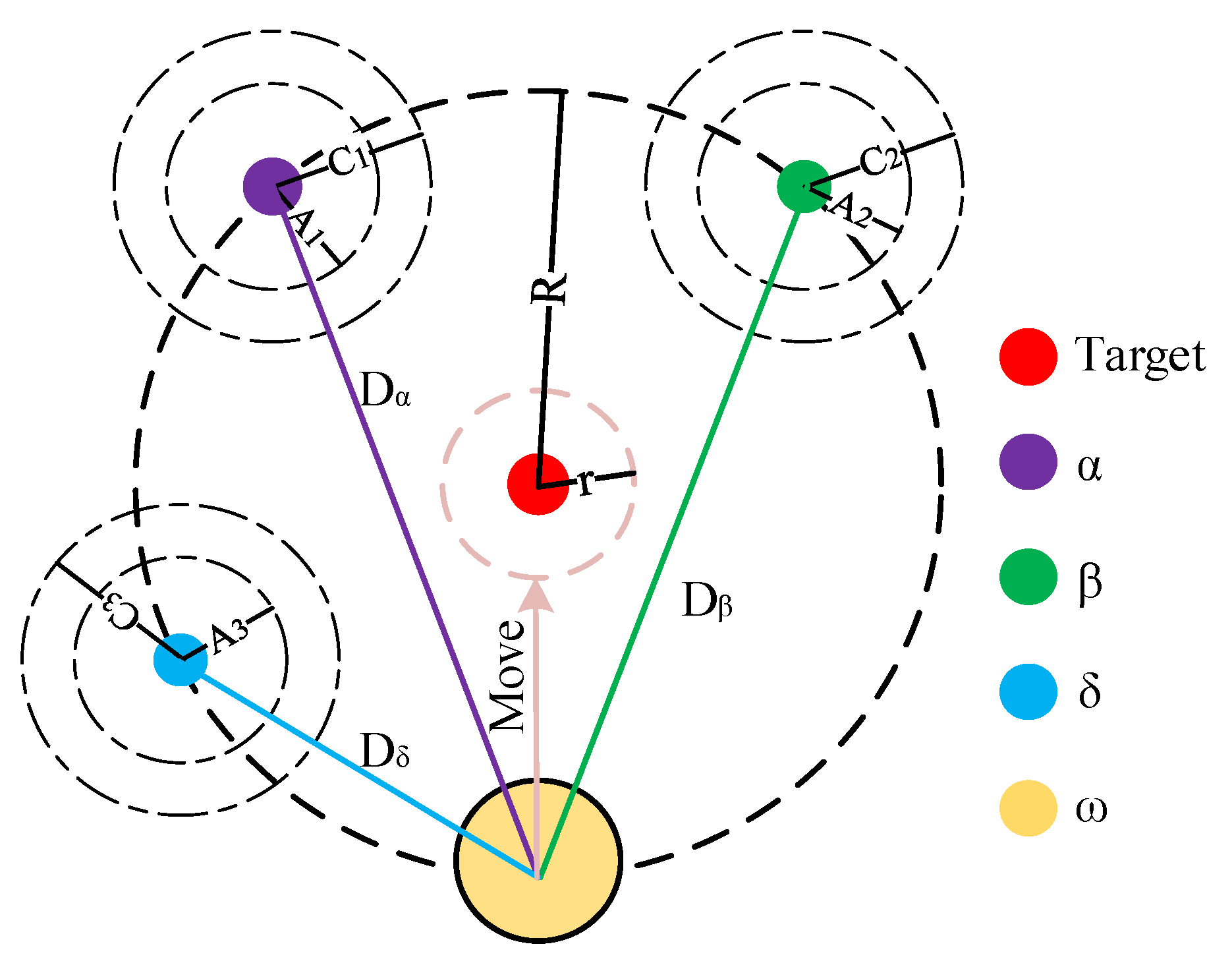
Figure 1. The diagram of gray wolf hunting.
Energies 14 05752 g001
Figure 2. The pseudo code of the SiGWO algorithm.
Energies 14 05752 g002
Figure 3. The pseudo code of the hybrid local search.
Energies 14 05752 g003
Figure 4. Main flow chart of the proposed algorithm.
Energies 14 05752 g004
Figure 5. The fitting curve of the predicted power.
Energies 14 05752 g005
Figure 6. The chart of error–time comparison.
Energies 14 05752 g006
Figure 7. The resource occupancy of power prediction.
Energies 14 05752 g007
Figure 8. The distribution diagram of RMSE.
Energies 14 05752 g008
Figure 9. Fitting diagram of the optimized predicted power.
Energies 14 05752 g009
Figure 10. The schematic diagram of the PV power generation system equipped with HESS.
Energies 14 05752 g010
Figure 11. The flow of advanced smoothing control strategy.
Energies 14 05752 g011
Figure 12. Power smoothing based on the predicted power.
Energies 14 05752 g012
Figure 13. The charge-discharge power of HESS.
Energies 14 05752 g013
Table 1. Evaluation indicators table.
Algorithm TypeMAPERMSETime
HLSGWO-LSSVM0.03%0.44%1.87 s
QPSO-LSSVM0.05%0.79%29.55 s
ABC-LSSVM0.13%1.94%46.72 s
SaDE-GWO-LSSVM0.16%2.42%54.31 s
Publisher’s Note: MDPI stays neutral with regard to jurisdictional claims in published maps and institutional affiliations.