1. Introduction
Boosting the annual energy extraction of wind turbines has been an important focus of wind energy researchers. Increasing the swept area of a wind turbine is a well-established study option. Since 1951, when the first wind turbine was connected to the grid, attempts to increase the size of rotors have increased [
1]. Another way to extract more wind energy is the insertion of a rotor of a wind turbine in a duct. Ducts can also be applied to airborne and windmills [
2,
3]. A wind turbine located within a duct is referred to as the Diffuser Augmented Wind Turbine (DAWT). It is also known as a ducted or a shrouded wind turbine. This turbine is installed within the circular section that causes an increase in the mass flow to the rotor due to its sectional circulation. Thus, the power extracted by the turbine increases, and the Betz limit can be surpassed both in terms of the rotor and duct-exit area [
4]. The additional advantages of DAWTs are the decreased cut-in speed, the minimized tip losses [
5], and noise [
6]. Additionally, there are the benefits of low sensitivity to variations of the yaw angle [
7], and the prospects for use in airborne applications for harnessing the stable and strong high-altitude wind streams [
3,
8], as well as installations in an urban environment [
9,
10]. Several investigations have been conducted experimentally and numerically for evaluation of the performance, the torque, and the thrust of DAWTs [
11,
12]. Moreover, DAWTs with auxiliary slots, high-lift compact DAWTs, conical DAWTs, and ground-based DAWTs have been considered in previous studies [
13,
14]. Ohya and Karasudani proved experimentally that inserting a horizontal axis wind turbine within a duct can increase the extracted power up to four times for some wind speeds [
15].
Heikal et al. [
16] studied the power coefficient (
) of a ducted wind turbine with numerical simulations. They reported a power factor of 90% for some wind speeds. Wind turbine ducts have different types and parts. For studying the wind turbine power increase due to ducts, it is necessary to examine various components of ducts. A duct may contain a nozzle, a diffuser, and a flange. The combined effects of these components on performance are not clear and only a few aspects have been investigated. In the study by Rochman et al. [
17], only the geometry of the flange of the duct was examined, which showed that adding a flat flange at the end of the duct causes an increase of 29% of wind speed in the throat region of the duct in comparison to the case without a flange. The studies of Ranjbar et al. [
18] and Al-Zahabi et al. [
19] focused only on the angle of a flange. Al-Zahabi et al. showed that, for their selected geometry, by setting the angle of the flange at 15 degrees, the power coefficient can be increased up to 5%. Ranjbar et al. demonstrated that if the duct is connected to a nozzle, the throat velocity can be enhanced up to 5.4%. The most prominent study of the effects of the angle and the length of diffusers can be found in the work of Ohya and Karasudani [
15]. They tested four ducts with different diffuser lengths. They showed experimentally that increasing the length of the diffuser makes reaching high wind speeds in the throat region of the duct possible. Kosasih and Tondelli [
20] studied both the length of the flange and the length of the diffuser. In the examined cases, they proved that the flange length increment made an increase in the wind velocity of the throat. On the contrary, the increased length of the diffuser resulted in a reduction of the ultimate power coefficient of the turbine located in the duct.
Wang et al. experimentally investigated the aerodynamics performance of a Vertical Axis Wind Turbine (VAWT) inside a diffuser. The diffuser increased the maximum generated power up to 26.31% [
21]. Watanabe et al. [
22] had experimental investigations of a ducted VAWT. Their optimization was based on changing the lengths and angles of the diffuser and flange. They also performed a parametric study on chord length, blade thickness, solidity, and Reynolds number. As they reported, the power extraction was doubled. Ghazalla et al. [
23] searched a proper location for the rotor inside the duct. The best position was the throat of the duct with the smallest cross section. Zanforlin et al. [
24] studied bi-directional symmetrical diffuser VAWTs at different yaw angles. The power coefficients of bi-directional symmetrical diffuser VAWTs were higher than a bare turbine at any yaw angle. Hashem and Mohamed [
25] used a Darrieus VAWT with three different types of the duct. They compared a flat-panel duct, a curved-surface duct, and a cycloidal-surface duct and showed the rotor covered with the cycloidal-surface duct generates the most power. Amgad et al. [
26] investigated the aeroacoustics and aerodynamics of a ducted VAWT. The results indicated that a velocity increase in the throat of the duct can augment the power coefficient by about 82%, which results in noisier operation. The urban integration of diffuser VAWTs was presented by Zanforlin and Letizia. They installed VAWTs inside a roof-and-diffuser system and showed that the power can be enhanced by about 40% rather than a case without a diffuser [
27].
One of the complicated phenomena for blade studies is dynamic stall. The sudden increase of the aerodynamic loads results in problems for the performance of wind turbines [
28,
29,
30,
31]. Although for horizontal axis wind turbines, the dynamic stall can be controlled, for vertical axis ones, these phenomena always exit [
32,
33] and should be considered.
The angles of the nozzle, diffuser, and flange as the main components of the duct play an important role to increase the wind speed inside the duct. Here, the angle optimization of these three components of the duct was considered, which had not been studied before to the best of the authors’ knowledge. The optimum angles will be achieved when the velocity inside the throat of the duct reaches its maximum value. A code has been developed to perform numerical simulations automatically. Then an H-Darrieus rotor was simulated inside the optimum duct. The power coefficient increment and the flow structure were investigated in detail. For the previous studies, the dynamic stall phenomena were investigated for ducted vertical wind turbines in detail, which were considered here.
2. Geometry and Numerical Approach of Duct Study
For the governing equations of the numerical approach, the continuity equation derived from the conservation of mass law and the total net flux of the control volume in the tensor form is
while the time-dependent term of the equation,
, is zero. To describe the fluid interaction, Navier–Stokes equations were used. The tensor form of these equations is given by
where
,
,
P, and
present the velocity, fluid density, static pressure, and dynamic viscosity, respectively. In Equation (2),
Gi, body force, is ignored because of its negligible value. The flow is considered two-dimensional and incompressible.
For solving full-elliptic Navier–Stokes equations,
k-
ε and
k-
ω models were used. According to the previous studies [
18,
19,
34], these two models can provide reliable results for flows around a rotor located in a duct. Two models were tested, and the
k-
ω model was selected [
35].
The finite volume method was applied. The governing equations were calculated via SIMPLE for the optimization part. For the simulation of the wind turbine with and without the duct, PISO was utilized. The discretization of equations was based on the second-order upwind method. The convergence criterion of the numerical simulations was for all equations. This threshold was absolute and a residual normalization was done.
Various types of ducts were designed and built for wind turbines. The duct used in this study was the duct provided by Ohya et al. [
15,
36]. This duct consisted of three parts: a nozzle, a diffuser, and a flange. The aim of using the duct was to increase the extracted power of the wind. The duct increases the kinetic energy of the flow by raising the wind speed in the throat region [
37]. Each part of the duct plays an effective role in increasing the flow velocity in the throat. The nozzle increases the cross section of the input, the diffuser enhances the flow velocity profile in the throat, and the flange creates a low-pressure region by creating strong vortices downstream of the duct. The downstream, low-pressure area creates a pressure difference between upstream and downstream of the duct. The pressure difference results in the flow velocity and the kinetic energy increments in the throat, where the turbine is installed [
38]. Considering the mentioned geometry shown in
Figure 1, the effective factors are the angles of these three parts. In
Figure 1, the nozzle (α), the diffuser (β), and the flange (γ) are shown. In the current study, to determine an optimum angle for each part, the lengths of the nozzle, diffuser, and flange were assumed constant with the values of 0.3D, 1.3D, and 0.3D, respectively.
Since the two-dimensional section of the duct is symmetrical, instead of simulating the entire domain, only half of it was considered as the numerical domain. Decreasing the size of the domain reduces computational costs. Although this simplification has been used and verified by other researchers [
39], the authors also solved the complete domain and compared the results. The top wall had the slip wall condition, which reduced the influences of the shearing stress [
39]. For the boundary conditions of the inlet and outlet of the domain, the velocity inlet and the pressure outlet were considered, respectively. The inlet velocity was equal to 8 m/s for all duct simulations. This velocity was considered as the reference velocity for making the flow parameters dimensionless. The wall and the inlet and the outlet of the domain were located far enough from the duct to reduce the effects of the boundaries on the duct.
Quadratic meshes were generated inside the computational domain (
Figure 1). The growth rate of the mesh length in the walls was 1.8. The maximum y+ values were less than 3 except in some limited cells close to the walls, which were about 8. For getting the optimum geometry of each component of the duct, all parts were needed to mesh separately in their blocks. Mesh independence was important for providing proper answers. Since the optimum angles of the duct were not accessible before optimizing the duct, the angle values of the nozzle, diffuser, and flange were considered as 11, 12, and 90 degrees, respectively, based on the study of Ohya et al. [
15,
36]. In
Figure 1, the number of cells examined for the duct is from 14,400 to 76,000 cells. The average flow velocity in the throat was dimensionalized with the reference velocity (8 m/s). From the results, meshes with 70,000 cells were independent. Increasing the number of cells caused around 4.14% velocity deviation. Considering the computational cost, meshes with 70,000 cells were selected.
For ensuring a reliable numerical simulation, the results were validated against the experimental data provided by Ohya et al. [
15,
36]. The experimental setup had no nozzle, shown in
Figure 1, and the same structure was applied for the numerical simulation. The non-dimensional velocities were measured in the central line of the duct. X is the centerline axis of the duct. L is the length of the diffuser. The diffuser starts at X = 0. The flange is located at X = L with an angle of 90 degrees. Two turbulence models
k-
ω and
k-
ε were applied. The comparison indicated that the
k-
ω model had less error than the
k-
ε model. For the
k-
ω model, the maximum discrepancy of the results compared to the experimental results was around 5%. Therefore, the
k-
ω turbulence model was used for the rest of this study.
4. Ducted Wind Turbine: Numerical Approach
Experimental and numerical investigations on bare wind turbines have shown that their maximum power coefficient is in the range of Betz-limit [
45,
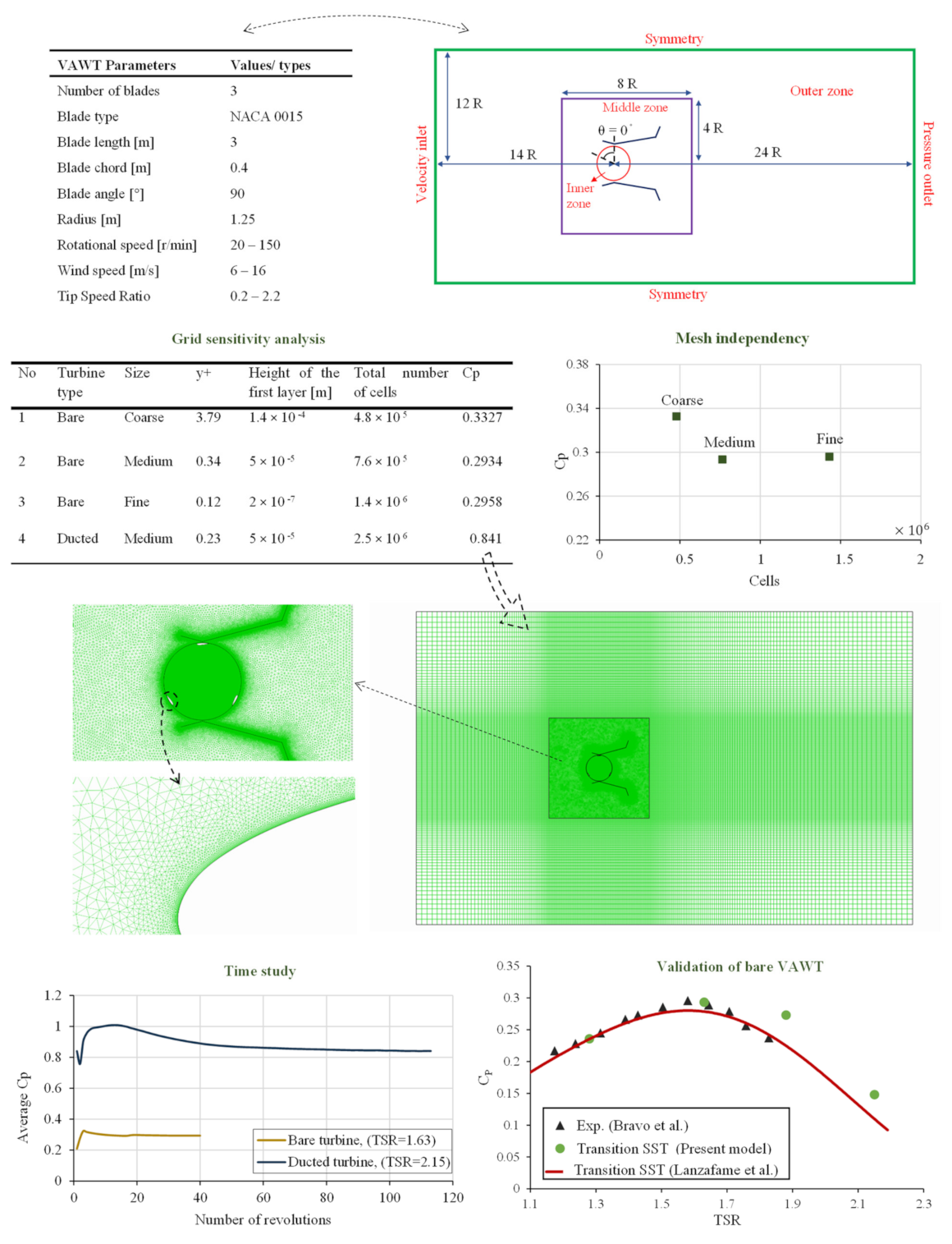
46]. In order to investigate the effects of the duct on the performance of wind turbines, two simulations of a VAWT with and without the duct were done. The bare turbine was an H-Darrieus wind turbine, according to Bravo et al. [
47] (
Figure 3). The blade angle was an angle between the chord of the blade and the radius of the rotor. Since the chord of each airfoil was always tangential to the rotor, the blade angle was 90 degrees. The duct with optimum geometry presented in
Figure 2 was considered. Since the H-Darrieus wind turbine inside the duct had a diameter of 250 cm, the lengths of the nozzle, the diffuser, and the flange were considered as 75 cm, 275 cm, and 75 cm, respectively. The length of the throat was 277.5 cm. To insert the rotor inside the duct, the clearance between the rotor and the duct was considered. In ducted turbines, the gap between the duct and the tip of the blade has an important role. Since there is a low-pressure region inside the diffuser, there is a possibility of stall. This gap creates a highly energetic jet that helps to attach the flow against the adverse pressure gradient flow at the boundary layer of the diffuser [
48,
49]; it recovers the pressure gradient and prevents the stall [
50].
The inlet boundary condition was considered velocity inlet with a constant value of 10 m/s and the outlet boundary condition was pressure outlet. The upper and lower boundary conditions were considered symmetry. To define rotational motion, the Sliding Mesh Motion (SMM) was considered in the inner cell zone. Boundary conditions and the computational domain are shown in
Figure 3.
The two-dimensional, transient, and incompressible equations, the continuity equation derived from the conservation of mass law, Equation (1), and the Navier-Stokes equations, Equation (2), were used. Standard
k-
ε,
k-
ω and transition Shear Stress Transport (SST) turbulence models were tested by Lanzafame et al. [
51]. Their results showed that the transition SST model has a good agreement with the experimental data, so this model was used in the present simulation.
The governing equations were calculated via Pressure-Implicit with Splitting of Operators (PISO). The second-order upwind method discretized the equations.
The flow domain of the ducted wind turbine was divided into inner, middle, and outer zones (
Figure 3). The flow domain for the bare turbine had just the inner and outer zones. At first, mesh-sensitivity analysis for the bare turbine was done with three sizes, named as coarse, medium, and fine (
Figure 3). The discrepancy between
of the coarse mesh and the fine mesh was 12.5%; this difference between the medium mesh and the fine mesh was decreased to less than 0.8%. In order to reduce the computational cost, the medium size mesh (7.6 × 10
5 cells) with less than 1% error was selected. The y+ value around the blade for the medium mesh was much less than 1. The medium mesh was also applied to the ducted wind turbine and showed the y+ value less than 1. For the inner zone, where the rotor was inserted, triangular meshes were generated. A boundary layer mesh with a growth rate of 1.1 from the walls of each blade in the interior zone was applied. This boundary layer consisted of 12 layers, with the first layer thickness of 5 × 10
−5 m. The middle zone with a square boundary covered the duct. Triangular meshes with a growth rate of 1.05 were generated inside the middle zone. The outer zone was fully covered by quadratic structured meshes.
In
Figure 3, the average power coefficients are plotted versus the number of cycles. The optimum number of cycles for the ducted turbine was about 85–90 and for the bare turbine was 28–30 cycles. The duct flow study showed that the velocity was oscillating in the throat because of the vortex shedding in the wake. In this regard, the number of revolutions required to stabilize for the ducted turbine was higher than that for the bare turbine, which agrees with the results of Zanforlin and Letizia [
27]. Moreover, higher angular velocities of the rotor increased the number of required revolutions.
For the numerical verification, the current numerical results were compared with the experimental results provided by Bravo et al. [
47], and the numerical transition SST results were presented by Lanzafame et al. [
51]. The power coefficients,
, of the bare wind turbine versus the tip speed ratio (
TSR) are shown in
Figure 3.
TSR is calculated as
.
is the free stream velocity (or inlet/reference velocity), 𝜔 is the angular velocity, 𝑅 is the rotor radius, 𝑃 is extracted power, 𝜌 is fluid density, and 𝐴 is the rotor area. The comparison indicated that the current numerical results followed the trend of the experimental data of [
50] and the numerical data of [
51]. It showed that the transition SST turbulent model can capture the trends of the experimental data perfectly, which was also reported by [
51].
5. Ducted Wind Turbine vs. Bare Wind Turbine
The aim of the study was the power coefficient increment of the VAWT using a duct. The power coefficients from the wind turbine were compared with those from the wind turbine located inside the optimized duct (
Figure 4). The power coefficient obtained from the ducted VAWT was much higher than the bare one. The maximum value of the power coefficient 0.84 occurred at the
TSR of 2.15. Using a duct, the extracted power of the wind turbines was improved in the other studies, too [
22,
25]. Watanabe et al. [
22] studied some ducts with different geometry and showed a power coefficient increment by 2.6 times more than an open wind turbine. Here, the maximum power coefficient was enhanced up to 2.9 times and postponed to a higher
TSR, which agrees with the study of Watanabe et al. [
22]. For some places, such as free spaces between tall buildings, the direction of the wind is almost constant. Where the direction of the wind does not vary significantly using ducted VAWTs is recommended to generate more power.
The inlet streamlines around the blades were platted at an azimuth angle of 30 degrees. The streamlines showed that the nozzle converged the input freestream flow and enhanced the incident velocity on each blade; the width of the stream-tube at the throat was decreased compared to that at the inlet. It was shown that the throat cross-section velocity was increased by 1.97 times when the duct was used. The dimensionless velocity and pressure coefficient contours for the ducted turbine and the bare turbine are shown in
Figure 4. The flow velocity in the ducted turbine domain was higher than that in the bare turbine domain. More pressure coefficient differences between the sides of the blades also proved that the aerodynamic loads were increased for each blade when the rotor was covered by a duct. Therefore, the blades of the ducted turbine generated a higher torque than the blades of the bare turbine.
As shown in the streamlines of the ducted turbine in
Figure 4, the walls of the duct caused vortex generation, such as the vortex marked with a blue box. When a rotor was inserted inside the duct, the horizontal and vertical components of the velocity were changed. As the rotor rotated, a low-pressure region was formed inside the bottom side of the diffuser causing an adverse pressure gradient; the flow separated, and some vortices were generated and shed to the wake periodically.
In
Figure 5, the power-coefficient comparison of a single blade between the bare and ducted turbines showed that the ducted turbine experienced a higher power coefficient in the azimuth angles of 0–90 degrees. For VAWTs, each section of the blade experienced a different angle of attack (AOA) during one rotation of the turbine. For the bare wind turbine, the AOA was oscillating [
52].
The AOA oscillation,
Figure 5, resulted in dynamic stall (DS) phenomena. DS phenomena of wind turbines can be studied by an oscillating airfoil [
28]. In this regard, besides the power extraction, the vortical structure of a blade can show valuable information for the rotor study. Since a leading-edge vortex is a very low-pressure vortex, the existence of the vortex on the suction side results in a high-pressure difference between the two sides of the airfoil and higher aerodynamic loads [
26].
Figure 5 also shows the vorticity fields of the bare and ducted wind turbines at the
TSR of 1.88. The flow structure from
Figure 5a,b shows that the AOA of the airfoil was increasing through turbine rotation, which resulted in enhancing the lift and drag loads [
28]. In
Figure 5b, a small, leading-edge vortex is visible for the ducted turbine. The formation of the leading-edge vortex as the main characteristic of DS resulted in the power coefficient reduction of the blade. After 10° rotation of the rotor (
Figure 5c), for the bare turbine, the first leading-edge vortex was seen, while the leading-edge vortex of the ducted one was more developed. There was also an approximately 10 degrees’ azimuthal angle difference between the first maximum blade power coefficients of the bare and ducted blades, which agrees well with the leading-edge vortex generation. Thus, the duct caused advancing dynamic stall vortex generation of the blades. In
Figure 5d,e, the leading-edge vortex development is visible for both turbines. Based on the developed leading-edge vortices, for both cases, the deep dynamic stall phenomena happened. In
Figure 5f,g, the leading edge vortices are separated from the blades, while the AOA is decreasing.
Figure 5h,i display that the airfoil experienced low angles with vortex sheets around the airfoil. Now, the dynamic stall loop was completed for both cases. Although the high wind speed through the throat passing the airfoil of the ducted turbine resulted in an improved power coefficient, the dynamic stall vortices including the leading-edge vortex caused power coefficient reduction. In sum, the wind turbine experienced a higher power coefficient when it was located inside the duct.
6. Conclusions
For a DAWT, the optimum angles for three components of the duct consisting of the nozzle, the diffuser, and the flange were established. A code was developed whereby, for each case, a geometry was introduced, and a structured mesh was generated automatically; then each case was solved numerically. The DOE and Kriging methods were used to estimate the output parameters based on input variables. The maximum error of numerical results using the k-ω model in comparison with the experimental results was 5%. Finally, the optimum angles of 15, 15, and 70 degrees for the nozzle, the diffuser, and the flange, respectively, gave the highest flow velocity in the throat. The average velocity of the throat was increased by 1.97 times in the optimum duct. The velocity distribution in 90% of the throat area was almost uniform, having the maximum kinetic energy of the flow. Since the dimensionless values for the duct lengths are provided, the results may be used for other studies.
The second part of this study was related to placing the H-type rotor in the throat of the optimum duct. The maximum power coefficient reached 0.84 at the TSR of 2.15. The power coefficient of the ducted wind turbine was increased 2.9 times compared to that of the bare wind turbine. The TSR associated with the optimum power coefficient was shifted 0.52 units for the ducted wind turbine.
The vortical structure of the rotors revealed deep dynamic stall phenomena. The numerical simulation captured all the details of the phenomena. A comparison between the bare turbine and the ducted turbine showed that the dynamic stall leading-edge vortex generation was advanced and its separation was postponed when the rotor was located in the duct. Although dynamic stall resulted in declining performance of the turbine, the overall flow change inside the duct enhanced the generated power of the ducted wind turbine. It can be concluded that using a duct to cover the rotor of a wind turbine properly is an efficient way to increase the extracted power. The ducted VAWT is recommended for places with uniform wind directions.


 ,
, 


