Abstract
Two methods are currently available to estimate in a relatively short time span the subsurface heat capacity: (1) laboratory analysis of rock/soil samples; (2) measure the heat diffusion with temperature sensors in an observation well. Since the first may not be representative of in-situ conditions, and the second imply economical and logistical issues, a third option might be possible by means of so-called oscillatory thermal response tests (OTRT). The aim of the study was to evaluate the effectiveness of an OTRT as a tool to infer the subsurface heat capacity without the need of an observation well. To achieve this goal, an OTRT was carried out in a borehole heat exchanger (BHE). The total duration of injection was 6 days, with oscillation period of 12 h and amplitude of 10 W m−1. The results of the proposed methodology were compared 3-D numerical simulations and to a TRT with a constant heat injection rate with temperature response monitored from a nearby observation well. Results show that the OTRT succeeded to infer the expected subsurface heat capacity, but uncertainty is about 15% and the radial depth of penetration is only 12 cm. The parameters having most impact on the results are the subsurface thermal conductivity and the borehole thermal resistance. The OTRT performed and analyzed in this study also allowed to evaluate the thermal conductivity with similar accuracy compared to conventional TRTs (3%). On the other hand, it returned borehole thermal resistance with high uncertainty (15%), in particular due to the duration of the test. The final range of heat capacity is wide, highlighting challenges to currently use OTRT in the scope of ground-coupled heat pump system design. OTRT appears a promising tool to evaluate the heat capacity, but more field testing and mathematical interpretation of the sinusoidal response is needed to better isolate the subsurface from the BHE contribution and reduce the uncertainty.
1. Introduction
Thermal response test (TRT) is the most common field method to estimate the subsurface thermal conductivity (TC) and the borehole thermal resistance for ground-coupled heat pump systems (GCHP). Hot water is circulated within the borehole heat exchanger (BHE) in order to inject 50 to 80 W m−1 during conventional TRTs [1,2]. Low-powered tests (10 to 25 W m−1) can also be conducted with a heating cable, which can even reduce the uncertainty associated to the subsurface TC because of the facility to evaluate the heat injection rate [3]. On the other hand, borehole thermal resistance cannot be properly assessed with a heating cable test. Other than being very compact and needing only 120 V power, the heating cable unit can provide a TC profile of the ground with several temperature sensors at depth, or with a fiber-optic cable [4,5]. Moreover, it does not require a BHE since it can be performed in open wells, provided that water is present to ensure thermal contact with the subsurface. Electric cable with heating and non-heating sections were also tested, but significant free convection occurs in the pipe (or well) according to the Rayleigh number stability criterion, thus allowing only 15% accuracy in TC estimation [4]. TRTs are commonly carried out for 48 to 72 h with a constant power ([2] and references therein). However, heat injection can be changed over time for different purposes. For instance, TRTs with step heat injection have been proposed to determine the optimal heat rejection/extraction rates for GCHP [6]. Constant-temperature TRTs have also been studied in order to reduce the testing time, increase the accuracy of the TC estimation via the slope method, and avoid the need of fixing the subsurface heat capacity (HC) to evaluate the borehole thermal resistance ([7] and references therein). To this regard, even though the range of variability of HC among geologic media is quite limited [8,9,10], a change from 1.5 to 3.2 MJ m−3 K−1 influences the thermal diffusivity (TD; ±40%) and thus the evaluation of the borehole thermal resistance (±10–23%) via conventional TRTs. In turn, we approximated that this could affect the evaluation of the total drilling length of BHEs by ±6–7%, with an impact of 3–4% on the total cost of the system. Moreover, HC is a crucial parameter in the design of underground thermal energy storage (UTES) systems, because it defines the amount of thermal energy that can be stored into the subsurface ([11,12] and references therein).
To date, subsurface HC can be evaluated via: (1) laboratory analysis of rock/soil samples; or (2) measurement of heat diffusion from a constant heat injection test with temperature monitoring in an observation well. Option 1 ensures results with accuracy of ±10% [13], but several samples need to be collected in order to thoroughly characterize the subsurface, and results may not be characteristic of in-situ conditions. Option 2 can provide information representative of in-situ conditions, but a second well needs to be installed in the field at a short distance from the heat source (ca. 1–2 m). However, such observation well is unlikely useful after the test. Moreover, a long-lasting heat injection (4 days at least for a well 1 m apart) is necessary to induce a significant thermal perturbation to be measured. In this work, we hypothesized a third option by means of the so-called oscillatory thermal response test (OTRT) that was implemented in the field. We evaluated if inducing an oscillatory heat injection rate allowed to evaluate the subsurface HC by analyzing the smoothed amplitude and phase shift of the temperature response monitored in the same BHE. This third option can be carried out without the need of samples or observation wells. However, the analysis of the thermal response can be quite challenging due to heat storage in both the BHE and the ground, whose individual contribution is difficult to distinguish.
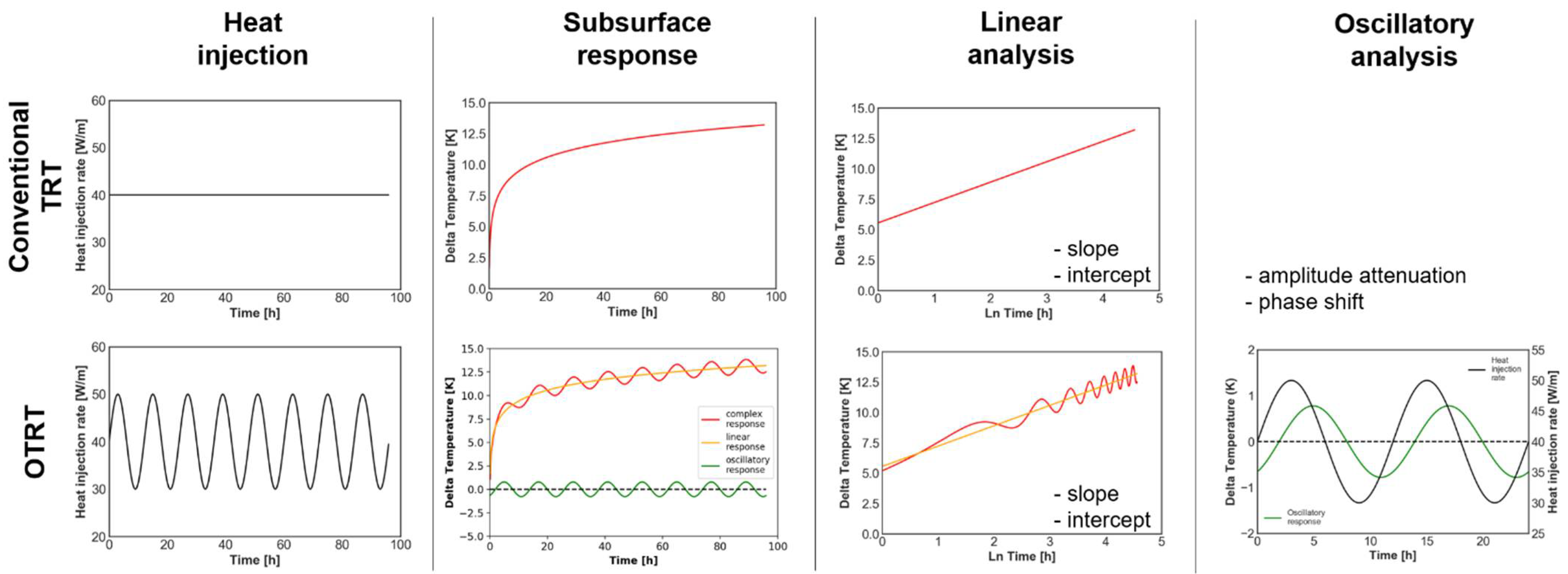
Oscillatory pumping tests (OPTs) have been used in hydrogeology as a practical and effective technique for establishing local-scale spatial variability in hydraulic parameters [14,15]. The phase shift and the amplitude attenuation of the recorded signal are functions of the transmissivity and storativity of the aquifer. The subsurface HC behaves similar to aquifer storativity [16]. Analogously, OTRT can be performed by inducing a heat injection sinusoid in a BHE, or a well, and measuring the sinusoidal thermal response of the system [17]. The use of an oscillatory heat source in replacement of a common constant power produces a sinusoidal signal whose phase and amplitude are affected by the storage of heat into the material surrounding the heat source. This provides more information about the subsurface and borehole thermal properties when compared to conventional TRTs. It is in the authors’ opinion that an OTRT might be useful to assess the subsurface TD (thermal analogue of the hydraulic diffusivity) and hence to estimate the HC, a property which cannot be evaluated via conventional TRTs. Indeed, the TRT methodology is based on the well-known transient infinite line source equation [18,19]. The heat injection is constant over time and the thermal response monitored in the same BHE is characterized by a constant temperature increase (semi steady state, [6]). A sinusoidal heat source equation needs to be used to reproduce temperature observations from an OTRT. In this case, the heat exchange rate between the borehole and the ground changes through time, and the temperature difference from the BHE pipe to the borehole wall also evolve with time, making the test difficult to analyze. The rate of temperature change that can be measured in a single BHE depends on both the HC of the BHE backfill material and the ground.
The objective of present study was to evaluate the effectiveness of OTRTs as a tool to estimate the subsurface HC in the scope of GCHP and UTES system design. First, 3-D numerical simulations were performed to validate the proposed methodology. Second, an OTRT was carried out with a water-circulation unit in a 154-m-deep grouted BHE equipped with a single U-pipe. In addition, an observation well was drilled 1.2 m apart from the BHE to evaluate the subsurface TD independently and assess the validity of the OTRT. A secondary objective was to evaluate if the OTRT can concurrently be used to assess TC and borehole thermal resistance with the same accuracy of conventional TRTs.
2. Materials and Methods
2.1. Research Hypothesis
According to [15] and references therein, periodic hydraulic testing (also called harmonic, oscillatory, sinusoidal) is a long-lasting measurement technique. It was used in the oil industry as early as 1966 and it was used in oil production wells with alternating periods of flow and shut-in during the 1970s. At the beginning, naturally occurring periodic oscillations such as Earth tides or barometric changes were used. The advantage is that these natural periodic variations affect the groundwater field over many kilometers. However, this natural phenomenon can be difficult to isolate and interpret due to the complexity of the superposition of different processes. Once performed on purpose, OPT can provide local hydraulic information about the aquifer, in particular about the spatial variability of transmissivity and storativity. By varying the oscillation frequency, different regions of the aquifer can be surveyed, and the special heterogeneity of properties is evaluated. While being valid for any type of aquifer, they are particularly effective in bedrock systems because a low storage coefficient provides a longer propagation of the signal from the test well compared to high storage coefficients associated to porous media. The amplitude and phase shift of the oscillatory response (drawdown) in the observation well compared to the sinusoidal source in the test well are function of the hydraulic conductivity (m s−1) and diffusivity (m2 s−1) ([14,15] and references therein).
Since the analogues of hydraulic conductivity and diffusivity in the heat problem are the TC and TD, the hypothesis is that the oscillatory thermal response induced by an OTRT brings information about the subsurface TD, and thus the HC (ratio of TC and TD, Figure 1). Differently from the hydraulic pumping tests, the use of an observation well is discarded due to both technical and financial reasons. First, the subsurface is a poor heat conductor. The duration of the test would be excessively long in order to induce a signal clear enough to be effectively analyzed. Second, the distance of the supposed observation well (short enough to reduce the duration of the test) would not be compatible with the conventional spacing adopted in bore fields of GCHP (6–8 m) or UTES (3–5 m), therefore making the observation well barely useful for the installation of shallow geothermal systems.
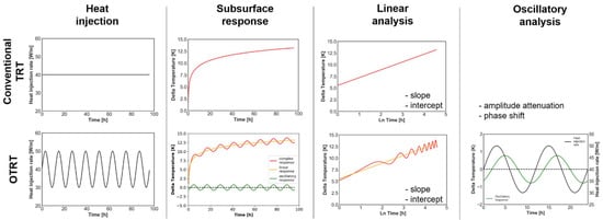
Figure 1.
Comparison between conventional and oscillatory TRT (reprint with permission [17]).
The main challenge with an OTRT is to incorporate in the analysis the influence of heat storage in the BHE backfilling material, commonly a sand-bentonite mixture or a thermally enhanced grout. Silica sand or groundwater can also be used if there is no risk of aquifer cross-contamination [20]. The storage effect due to the HC of the backfilling material plays a key role in the oscillatory signal propagation, thus limiting the depth of investigation (radial distance) of the OTRT. This has also been highlighted in OPTs, which are proved to be more effective in low-storativity settings such as bedrock aquifers [15]. The oscillation frequency of the OTRT is therefore a crucial parameter affecting the trade-off between the test penetration depth and duration that need to be chosen. To the best of our knowledge, Ref. [17] is the first and only study that performed an OTRT in the field. The results showed that high-frequency tests have small penetration depths and can highlight anomalous borehole thermal resistance due to flaws of the geothermal grouting. On the other hand, high-period tests (low frequencies) are necessary to increase the penetration depth to more than 10 cm and significantly affect the subsurface. A comprehensive description about the theory and analytical approach used to analyze the OTRT in this study are provided in the following Section 2.2.
The hypothesis of the research study being stated, the following steps were carried out to verify the effectiveness of OTRT for the estimation of the subsurface HC:
- To perform a constant-heat-injection TRT while recording the thermal response in a nearby observation well in order to have a first estimate of the subsurface HC;
- To perform 3-D numerical simulation to validate the proposed methodology
- To carry out an OTRT in a BHE and compare the HC results to those obtained in steps 1 and 2.
2.2. Oscillatory Heat Injection Theory and Analytical Approach for the Evaluation of Thermal Diffusivity
An oscillatory (sinusoidal) heat injection carried out in a BHE has the following form:
where (W m−1) is the heat injected per unit length, (W m−1) is the offset of the sinusoidal function, P (h) is the period of the oscillation and t (h) is time. This induces an oscillatory thermal response in the same well (, with borehole radius) which is described by the following equation given by Eskilson [21]:
where (°C) is the temperature at the borehole wall, (m K W−1) denotes the resistance opposed by the surrounding medium, and is therefore called oscillatory resistance, and (-) is the phase shift of the thermal response expressed as a fraction of P (0 < < 1). and can be evaluated by comparing the heat injection and thermal response as described by the following Equations:
where (K) and (W m−1) are the amplitudes of the thermal response and heat injection, respectively. Equation (2) is valid only if the system is linear time invariant, i.e., the oscillation frequencies of the heat injection and thermal response are the same, as described and demonstrated by [17]. If the heat source can be simplified to a heated line, there exists an analytical solution and Eskilson [21] derived the expressions for (Equation (5)) and (Equation (6)) as a function of , a dimensionless factor described in Equation (7) which depends on the depth of investigation (, assumed as the radial distance from the heated line, Equation (8)), which in turn varies according to the subsurface TD. Therefore, we have:
where (W m−1 K−1) is the subsurface TC, is the Euler-Mascheroni constant and (m2 s−1) is the subsurface TD. Eskilson’s expressions are approximated to the first terms of the Taylor series expansion of the Kelvin function. The validity of this approximation is further discussed in Appendix A. It is finally important to highlight that the oscillatory resistance depends on both the TC and TD of the subsurface (Equations (5), (7) and (8)), while is only function of the diffusivity (Equations (6)–(8)).
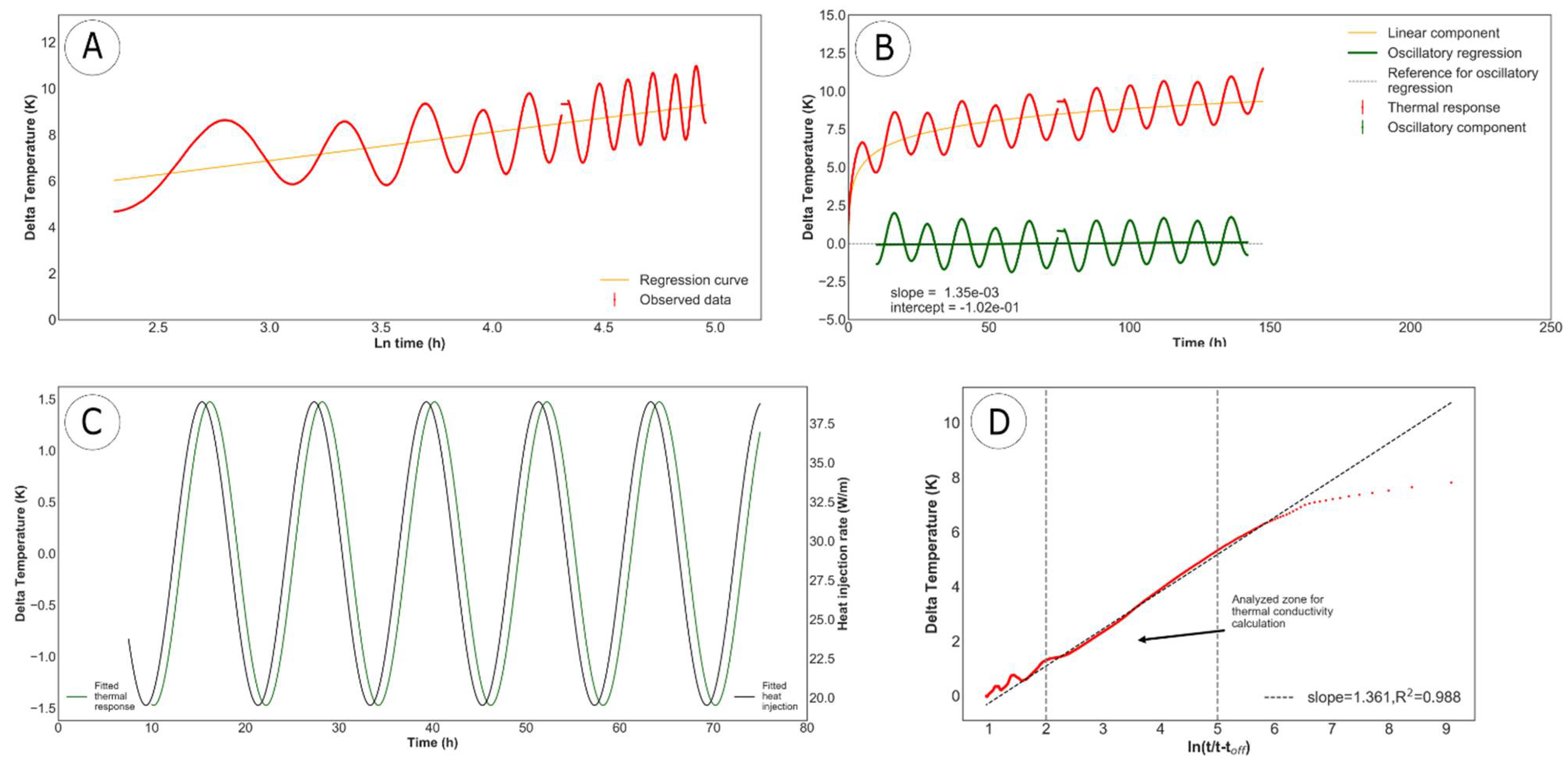
The proposed methodology for the analysis of the OTRT is carried out through the main following steps:
- Evaluation of TCheating and borehole thermal resistance via the slope method (Figure 2A, Ref. [2] and references therein);
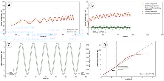 Figure 2. Steps for the analysis of an OTRT: (A) evaluation of λheating and via the slope method; (B) split of the linear and oscillatory components; (C) comparison of the oscillatory heat injection and the oscillatory thermal response; (D) analysis of the recovery period to estimate λcooling.
 - Subtraction of the linear component function of TCheating and in order to obtain the oscillatory component of the OTRT response (Figure 2B);
- Comparison of the oscillatory heat injection and the oscillatory thermal response to evaluate and . Evaluation of TD by means of the Equations (5)–(8) (Figure 2C);
- Analysis of the recovery period to estimate TCcooling, which we assume as the in-situ subsurface TC because it is not affected by the borehole thermal resistance ([22], Figure 2D);
- Evaluation of HC via the ratio TCcooling/TD.
Eskilson [21] suggested that Equations (5) and (6) are valid provided that , and thus . This means that an OTRT would have to last several days (p > 1000 h or 40 days) for the thermal front to reach the subsurface, which is clearly not practical and economically feasible. One key parameter in the calculation is the borehole radius, whose value in conventional 4.5-inch (0.057 m) and 6-inch (0.076 m) BHE is excessively high for Eskilson’s criterion to be respected. However, an equivalent radius can be considered such to account for the effect of the grout TC and the borehole thermal resistance as described by the following Equation ([23] and references therein):
where is the TC of the backfilling material in the borehole.
The methodology described above needs to be validated with periods of oscillation compatible with field test duration, otherwise Esklison’s analytical expressions would not be valid with common BHE radius. The use of an equivalent radius (Equation (9)) simplifies the BHE problem to a 1-D geometry. This allows us to fix the influence of the BHE heat storage (included in Equation (9) via and ) and consider a steady-state heat transfer within the BHE. More details about the validation of the methodology, and its simplifications and assumptions are reported in Appendix A and Appendix B, respectively. Results demonstrate that Eskilson’s expressions, together with the use an equivalent BHE radius, can properly be used to analyse OTRT with low periods of oscillation (12 and 24 h). The proposed methodology was therefore used to analyze both the numerical simulations and the OTRT conducted in the field as explained in the following.
2.3. Description of the Test Site
The test site is located at the Laboratoires pour l’innovation scientifique et technologique de l’environnement of the Institut national de la recherche scientifique (INRS), in the Parc technologique du Québec métropolitain (Québec City, QC, Canada). Geographical coordinates are N 46°47′44.58″ and W 71°18′09.97″. The bore field at the site is made of a 154-m-deep single-U BHE (1-U) and a 165-m-deep double-U BHE (2-U). Four observation wells are located in between the BHE along a NW direction parallel to the hydraulic channel nearby (Figure 3). OBS1, OBS2, OBS3 and OBS4 are 42, 42, 49 and 26-m-deep, respectively. A fifth well (OBS5), 15-m-deep, was also drilled at the eastern limit of the site in order to evaluate the local potentiometric field and evaluate the groundwater flow (GW) direction and magnitude. Local GW direction is NE with hydraulic gradient of 1.0 to 1.5%.
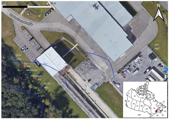
Figure 3.
Orthophoto view of the study site. BHEs and observation wells are indicated by red and blue dots, respectively. Numbers indicate the water level in meters above sea level (m a.s.l.), blue lines represent the local potentiometric field.
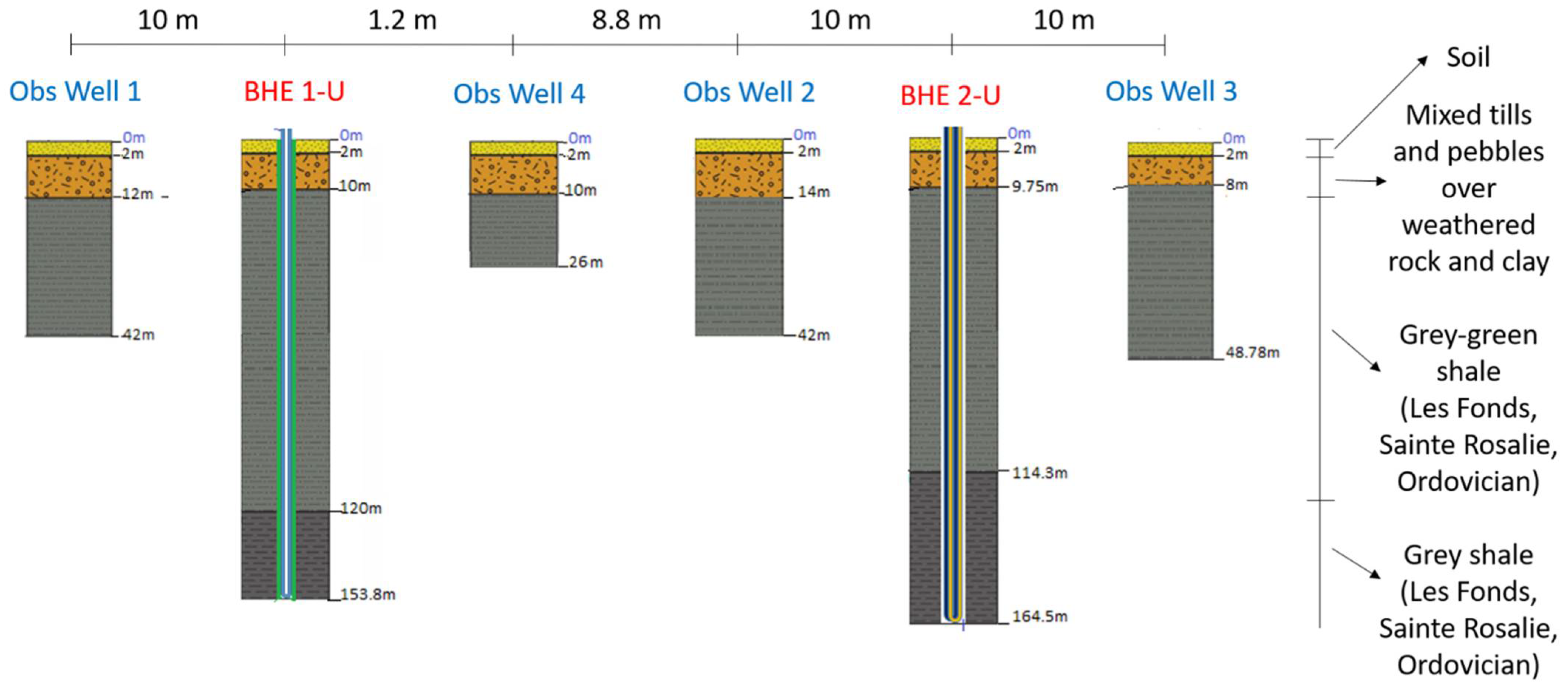
From the geological point of view, the local stratigraphy consists of 2 m of soil overlying 8 to 12 m of mixed till and pebbles, followed by clays over weathered rock (Figure 4). The bedrock is made of green and grey shales belonging to the Les Fonds Formation of the Sainte Rosalie Group, in the Saint-Lawrence Lowlands sedimentary basin [24]. Fracture zones were detected at depths of 20–25 m, 40–45 m, 95 m and 137 m during the drilling of the 1-U borehole. From previous TRT and slug tests carried out at the same site, bulk TC of the shales is 1.7–1.8 W m−1 K−1 and hydraulic conductivity of the highlighted fracture zones is 10−8 m s−1. Darcy flux was estimated to 1 to 4 × 10⁻⁹ m s−1, and Darcy velocity to 10−10 m s−1 [25,26,27]. Koubikana Pambou et al. [27] showed that GW does affect the subsurface TC inferred from TRT in correspondance of the fracture zones, with effective TC reaching maximum values of 2.0 W m−1 K−1. However, this influence appears to be local and limited to fracture zones with thickness of few meters. Therefore, the OTRT analysis is expected to be unaffected by GW in the chosen 1-U BHE at the study site. The volumetric HC of the shales is estimated to be in the order of 1.8–2.4 MJ m−3 K−1 from the literature [8,9,10]. The shallowest 10 m of the sequence are expected to have a lower TC and a higher HC due to the higher water-filled porosity of the deposits (see Figure 4).
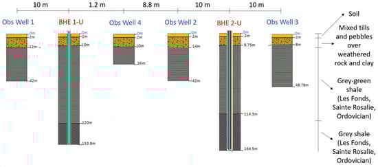
Figure 4.
Cross section of the study site between the observation wells 1 and 3.
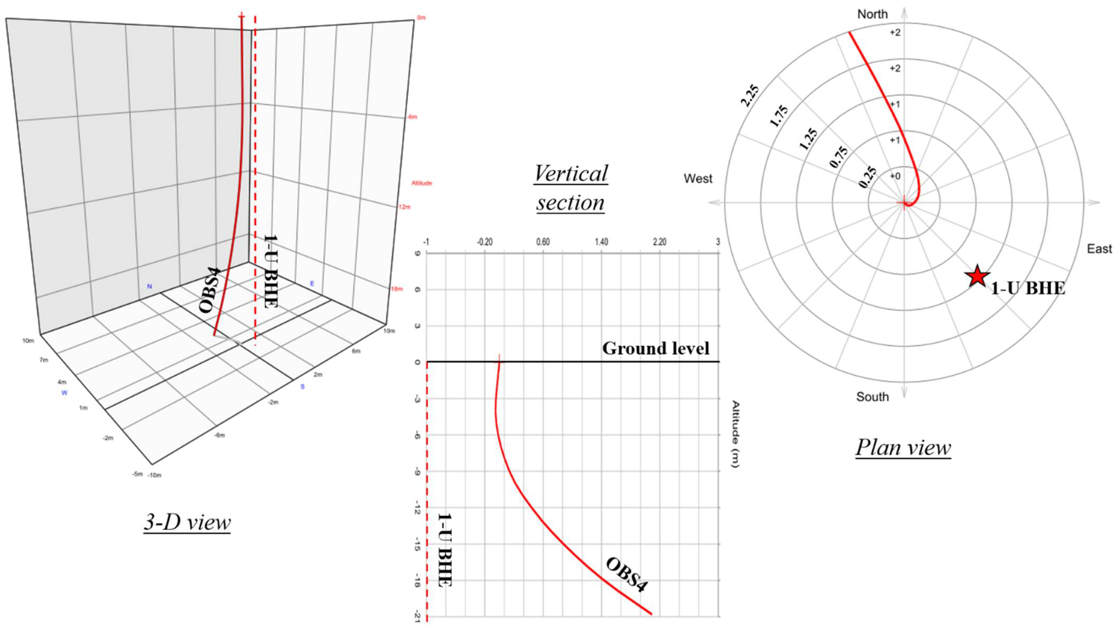
The BHE used for the present study was installed in the 0.114-m-diameter borehole (4.5-inch). The single-U pipe has no spacing clips and is made of high-density polyethylene, with nominal diameter of 1 inch (outside and internal radius are 0.021 m and 0.017 m, respectively) and a standard dimension ratio (SDR) of 11. Pipe TC is 0.48 W m−1 K−1. The backfill is a geothermal grout mixture with water, bentonite and silica sand, with nominal TC of 1.7 W m−1 K−1 (error 10%, [28]). The expected grout TD is in the order of 0.44 mm2 s−1. The fluid circulating in the BHE is water, with density of 1.0 × 10³ kg m−3, dynamic viscosity of 1.37 × 10⁻³ kg m−1 s−1, and specific heat of 4.2 kJ kg K−1. The observation well OBS4 (diameter 0.051 m, depth 26 m) was drilled on purpose for the present study beside the 1-U BHE, at a distance of 1.2 m. Drilling a hole parallel to the BHE was challenging as expected, since the general deviation of the inclination of boreholes ranges from 1 to 10% of the depth. In order to have two parallel holes, it would have been necessary to drill them one after the other, with the same drilling machine and same operator. However, drilling another BHE was not possible due to field constraints. To partially reduce uncertainty, the inclination of OBS4 was measured to know the actual distance between the supposed linear heat source (1-U BHE, assumed vertical) and the observation well (OBS4). The assumption of the vertical BHE appears reasonable since the hole has a larger diameter (more than 2 times), a longer depth and was drilled with heavier machinery. The inclination analysis of OBS4 was carried out with the Gyro Master probe by SPT Semm Logging (inclination accuracy ± 0.05°). Results show that horizontal deviations with respect to the vertical are 0.05, 0.2, 0.9 and 2.1 m at depths of 5, 10, 15 and 21 m, respectively (Figure 5). The well is almost linear down to 10 m, with slight eastward inclination, then the deviation rate becomes bigger, and the inclination tends towards NNW. Distances to the BHE, assuming the latter to be vertical, are approximately 1.2, 1.3, 2.0, 3.0 and 4.4 m at depths of 5, 10, 15, 20 and 25 m (projected), respectively.
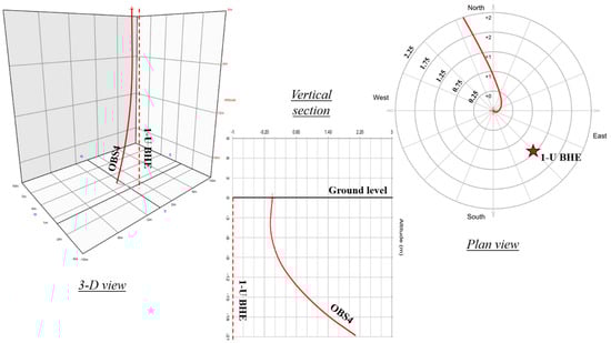
Figure 5.
Inclination of the observation well OBS4 (red line) and comparison with the projection of the 1-U BHE (red dashed line and star).
2.4. Numerical Simulations
Numerical simulations were carried out with the commercial code FEFLOW [29]. Three different scenarios were simulated with subsurface HC of 2.0, 2.4 and 2.8 MJ m−3 K−1, named SC1, SC2 and SC3, respectively. TC was set to 1.7 W m−1 K−1 in all scenarios, so subsurface TD is 0.85, 0.71 and 0.61 mm2 s−1, respectively. A test simulation demonstrated the negligible effect of the shallowest weathered unconsolidated sediments on the whole sequence. Therefore, only the shales were represented in the model in order to speed up the calculation.
The subsurface was modeled in a 100 × 100 × 350 m 3-D volume, discretized in 66,600 triangular prismatic elements. Grid independence validation was carried out to select the mesh element number as the best trade-off between computation time and stability of the results. The mesh refinement around the 1-U BHE respected the critical radius described by [30] in order to account for the real size of the BHE and ensure numerical stability. The BHE was assigned to an element edge and simulated as a linear element (1-D) immersed in the 3-D mesh. The BHE problem was solved with the quasi-stationary analytical solution proposed by [31]. This analytical solution is not recommended for variations in a time scale shorter than about 3.5 h due to the violation of the steady-state conditions [30]. However, the fully transient numerical approach proposed by [32] turned out to be highly unstable and computationally heavy, thus unsuitable for the present problem.
The specific BHE tool in FEFLOW was used to solve the heat transport equation, where a set of Dirichlet, Neumann and Cauchy-type boundary conditions are assigned to obtain the temperature at the borehole wall (, [30]). The power deduced from the field test experiment was set as input. According to [33], when using the quasi-stationary analytical solution to solve the BHE problem, FEFLOW uses the delta configuration described in the thermal resistance and capacity model (TRCM, [34]). A 1-U borehole configuration consists of four components (pipe-in, pipe-out and grout subdivided in two zones) and the resistances are calculated by FEFLOW via the TRCM model. However, if experimental results of the borehole thermal resistance are available, one can define the specific resistances linking each component of the BHE.
The borehole thermal resistance and the internal borehole thermal resistance were calculated via the multipole method [35,36] in order to match the experimental results from previous conventional TRTs carried out at the study site [26]. As demonstrated by Lamarche et al. [37], the multipole method proved to be the closest to numerical simulation results among the methods considered. The multipole method was judged the most suitable for our specific case since it takes into account the ratio and some geometric dimensionless parameters (Equation (9) in [37]). According to the nomenclature presented by [37], the equivalent or 3-D resistance was calculated as follows [38]:
with:
where H (m) is the BHE length, m (kg s−1) is the flow rate, (J kg−1 K−1) is the specific heat of the working fluid, and and are the borehole and internal resistances including the pipe resistance. With the BHE configuration having dimensions and characteristics described in Section 2.3 and a shank spacing of 0.028 m, and were evaluated to be 0.0798 and 0.3117 m K W−1, respectively. The equivalent resistance is finally 0.0894 m K W−1 (error 10%), in agreement with that found with in-situ assessment [26,28]. In FEFLOW, was assigned to the two pipe-grout and the grout-soil resistances. The grout-grout resistance () was calculated as follows [33]:
Surface temperature and geothermal heat flow were considered to have negligible influence on the simulation, and therefore not assigned. In addition, the model geometry was wide enough to avoid side boundary effects. In the light of the previous experiments, an initial temperature of 8 °C was assigned to all the elements of the model. After proper validation, groundwater flow boundary conditions were not assigned due to the negligible effect over the time span of the OTRT. Finally, the time discretization followed an automatic scheme in order to minimize the errors and reach the convergence.
2.5. Field Tests
2.5.1. TRT with Constant Heat Injection
In order to independently estimate the subsurface TD and compare it to the OTRT result, a constant-heat-injection TRT was carried out from the 10th to 14th of June 2019, in the 1-U BHE. The test was performed with a heating cable unit and a cable length of 22.5 m [3]. The heating cable technique was used because it is an affordable, easy and sound technique to infer the underground thermal conductivity as already demonstrated in the literature [3,4,5]. Submersible temperature sensors (accuracy 0.1 °C, resolution 0.032 °C) were placed along the heating cable at depths of 2.5, 5, 10, 12.5, 15, 17.5, 20 and 22.5 m from the ground level. Similar temperature sensors were installed in the observation well OBS4 at the same depths from 5 to 25 m. OBS4 was drilled 2 weeks before, and temperature profiles were measured in the BHE and the observation well itself such to wait for the undisturbed temperature to be recovered before starting the TRT. The idea was to analogously reproduce a dual-needle test commonly made on hand samples to determine the subsurface TD, but at the scale of a BHE. To analyze this field test, the thermal response of the subsurface at a distance was simulated using the thermal response functions developed for the infinite cylindrical source (ICS) and infinite line source (ILS) Equations [19] (and references therein).
2.5.2. OTRT
The OTRT was carried out with a conventional water-circulation unit from the 7th to 13th of July 2020. The TRT unit was made of a heating element located at surface with maximum power of 7 kW, a hydraulic pump, a flowmeter (0.5% accuracy) and temperature sensors (accuracy 0.15 °C, resolution 0.01 °C) placed near the pump in a trailer. The fluid (water) was heated in a reservoir in the trailer before being injected in the BHE. The heating power was then calculated via the BHE inlet/outlet temperature difference, the flow rate and the heat capacity of the circulating fluid (refer to Section 2.3 for the properties of water). Temperature controllers were used to adjust heat injection and ensure a sinusoidal heat injection rate. The equivalent borehole radius was calculated with grout TC 1.7 W m−1 K−1 and 0.09 m K W−1, and it turned out to be 0.022 m. This value was also used for the analysis of the numerical simulations results.
3. Results
3.1. TRT with Constant Heat Injection
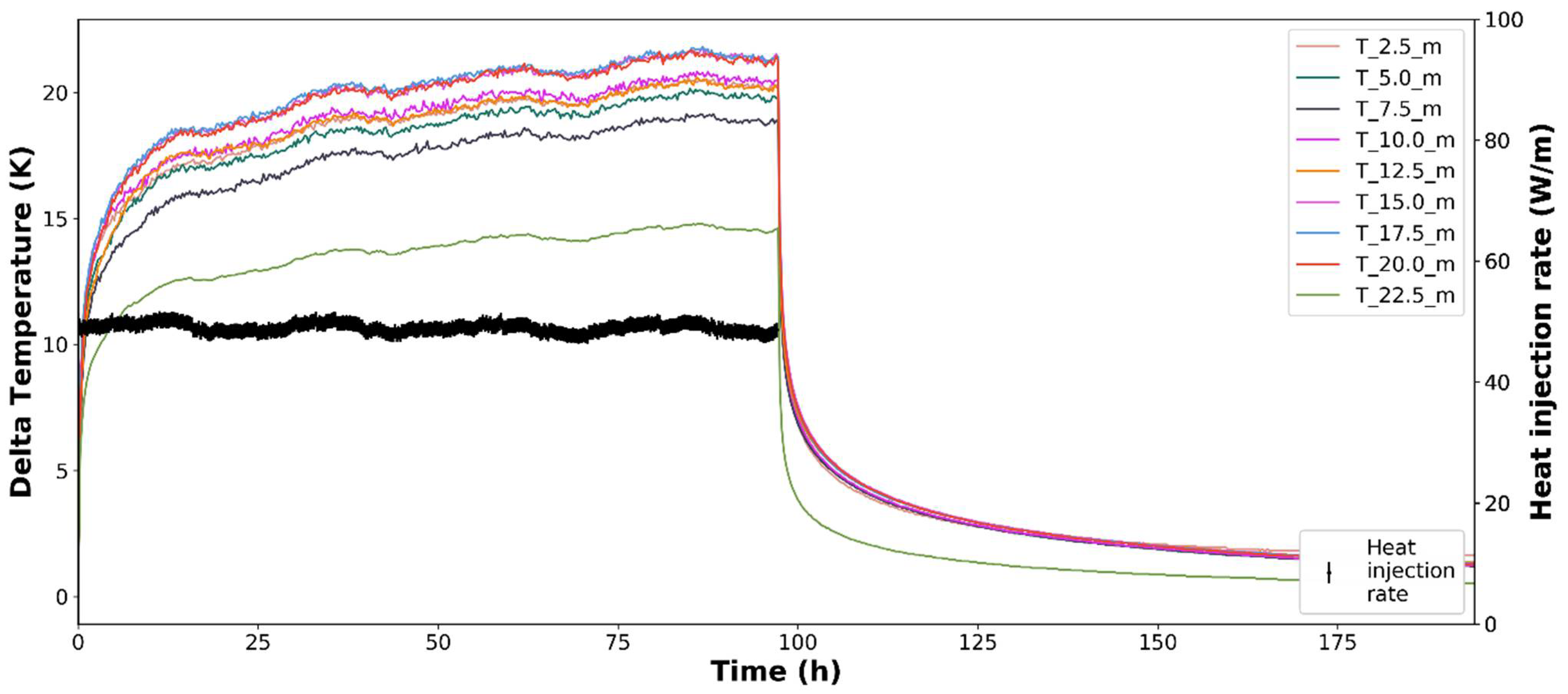
The constant-heat-injection TRT lasted 97 h with an average power injected of 48 W m−1 (Figure 6). The TC was evaluated via the recovery period in order to avoid the effect of the borehole thermal resistance and cable location, which can induce noise in the temperature signal of the heat injection period. This is because the heat source is placed in only one of the BHE pipes and thus its lateral position in the BHE slice remains unknown. The slope analysis of the recovery period outputs TC of 1.8–2.0 W m−1 K−1 from 5 to 20 m (Table 1). The error of the estimation δ (uncertainty) was calculated to be ca. 2.5% according to the methodology proposed by [39]. The results show a slight but clear difference in the first 10 m ( > 1.95 W m−1 K−1) compared to deeper portions ( < 1.95 W m−1 K−1), reflecting the local stratigraphy (see Figure 4). First and last sensors do not give reliable results due to violation of the ILS assumptions and the possible occurrence of convection cells. In particular, the last sensor shows a different behavior from the other sensors (see Figure 6). Therefore, they were not considered representative.
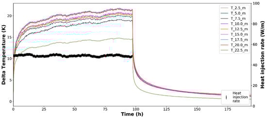
Figure 6.
Results of the constant-heat-injection TRT with heating cable in the 1-U BHE.

Table 1.
Thermal conductivity deduced from the recovery period for the constant-heat-injection TRT.
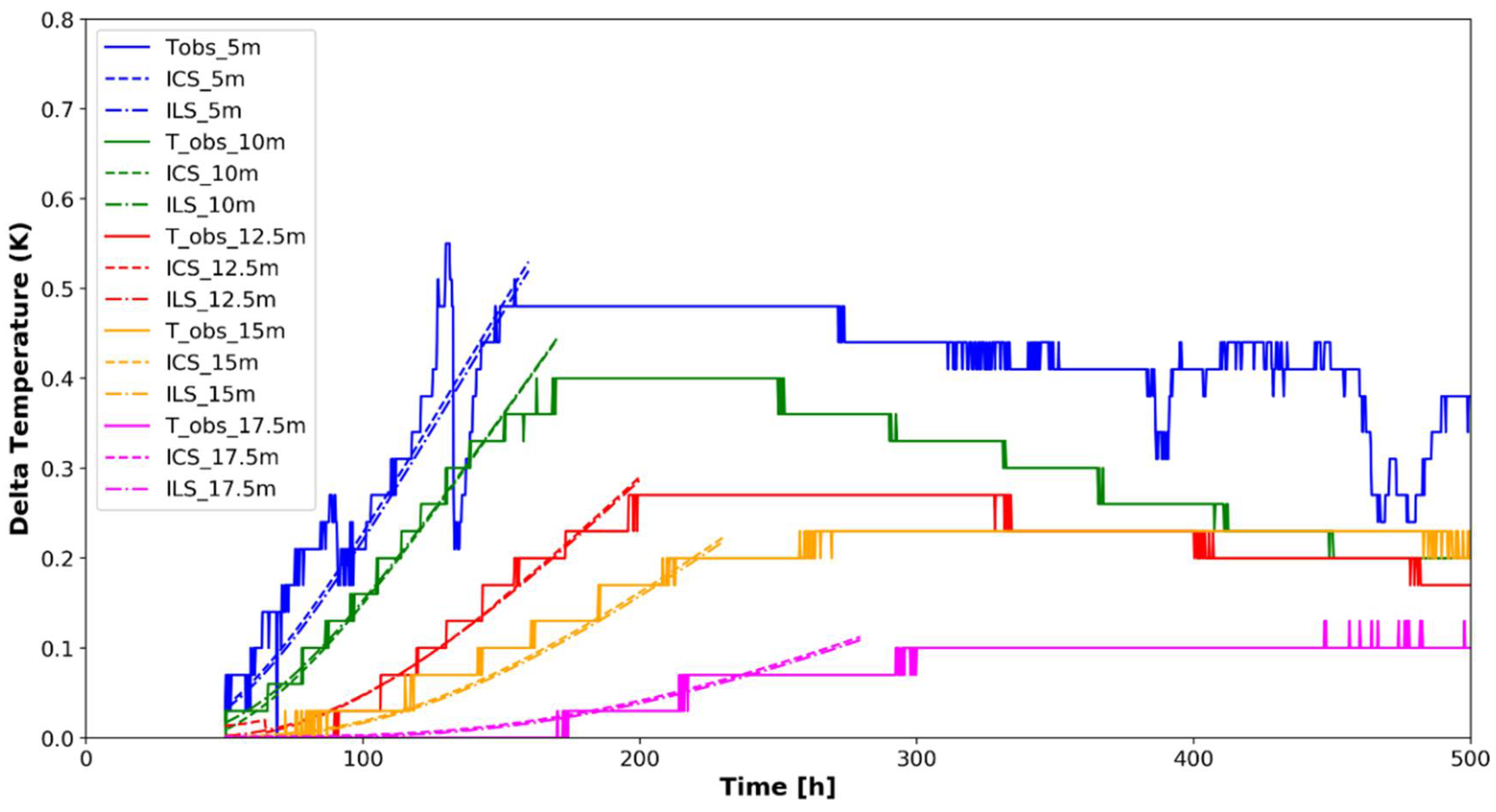
Temperature recordings in OBS4 are clearly affected by the inclination of the well, with the signal becoming smoother and smoother with increasing depth or increasing distance from the BHE (Figure 7). The thermal response recorded in the observation well shows a maximum temperature variation of 0.59 °C at 7.5 m depth after 160 h from the beginning of the test. The maximum values recorded at 10, 12.5, 15 and 17.5 m are 0.40, 0.27, 0.23 and 0.13 °C, respectively (Figure 7). Sensors below 17.5 m do not display a valid thermal response due to high distance ( > 2.5 m). This confirms the assumption that the BHE is vertical in the first 20 m below the ground, and that the distance between BHE and OBS4 is progressively increasing according to the magnitude and direction of the well inclination. Sensors from 5 to 17.5 m were analyzed to evaluate the TD (Figure 7 and Table 2). The observed data were manually matched by means of ICS and ILS response functions with TD values reported in Table 2. TD values are lower in the shallow sequence (0.70–0.75 mm2 s−1) and higher in the deep portion (0.77–0.82 mm2 s−1). The thermal response is therefore highly affected by the inclination of the observation well, i.e., the distance . Using the TC obtained through the previous analysis of the recovery period in the BHE, HC is found at the depth of temperature sensors. Finally, two thermo-geological units can be distinguished: the unconsolidated deposits in the top 10–12.5 m showing higher HC (2.7–2.8 MJ m3 K−1) and lower TD; the shale rock in its shallowest part showing lower HC (2.3–2.5 MJ m3 K−1) and higher TD (Table 2). TC is however similar in the two units.
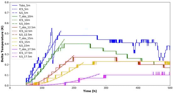
Figure 7.
Thermal response monitored in the observation well (T_obs) at 5 different depths, compared to temperature calculated with ICS and ILS response functions.
3.2. Numerical Simulations
The results of the numerical simulations, based on the field test conditions, show a clear different behavior among the selected scenarios (Figure 8). TC evaluated by matching recovery temperature simulated with the numerical model ranges from 1.68 W m−1 K−1 (SC3) to 1.71 W m−1 K−1 (SC1), while the borehole thermal resistance is 0.125 m K W−1. The overestimation of was expected due to the use of the analytical solution in FEFLOW. As shown by [30], the analytical approach overestimates the outlet BHE temperature in the first hours of simulation with respect to fully transient simulations, therefore raising the intercept of the linear regression.
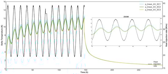
Figure 8.
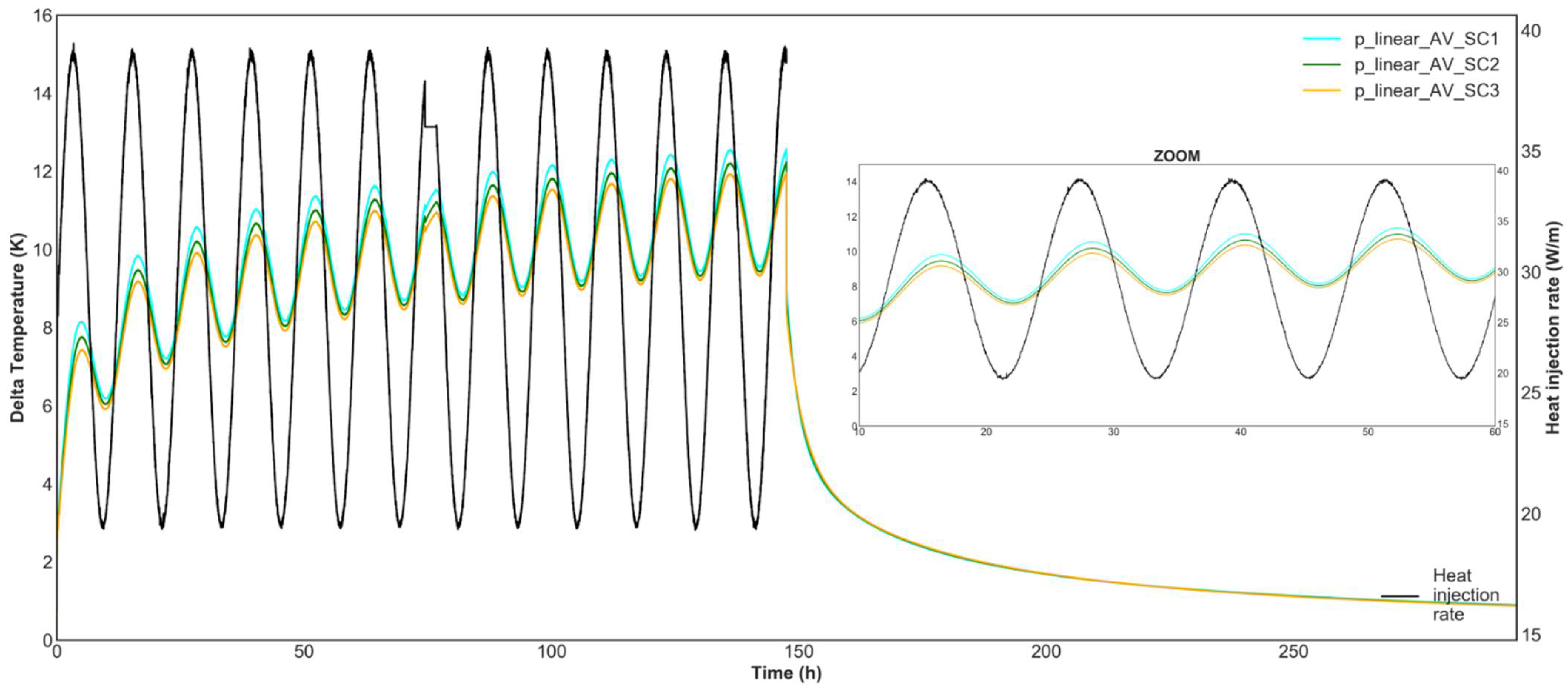
Numerical simulation of OTRT for the three subsurface scenarios.
inferred from simulated temperature ranges from 0.155 to 0.135, decreasing with increasing HC from SC1 to SC3. On the other hand, the phase shift does not present any significant difference among the scenarios, with at 0.11 in the three cases (Table 3). TD shows maximum deviation D (%) from the expected values of 25%, 9% and 2% in SC1, SC2 and SC3, respectively, when the estimation is carried out by means of the oscillatory resistance (Equation (5), Table 4). However, the TD estimation from the phase shift returns deviations > 30%. Similarly, the HC is evaluated with deviations < 20% through , and deviations > 50% through (Table 5). Interestingly, the higher the subsurface HC, the better the estimation of TD and HC.
Table 3.
OTRT parameters inferred from the numerical simulations.
Table 4.
Thermal diffusivity deduced from Equation (5) () and Equation (6) () with deviations from the input value.
Table 5.
Heat capacity deduced with TD from Table 4 and TC from the cooling period with deviations from the input value.
3.3. OTRT
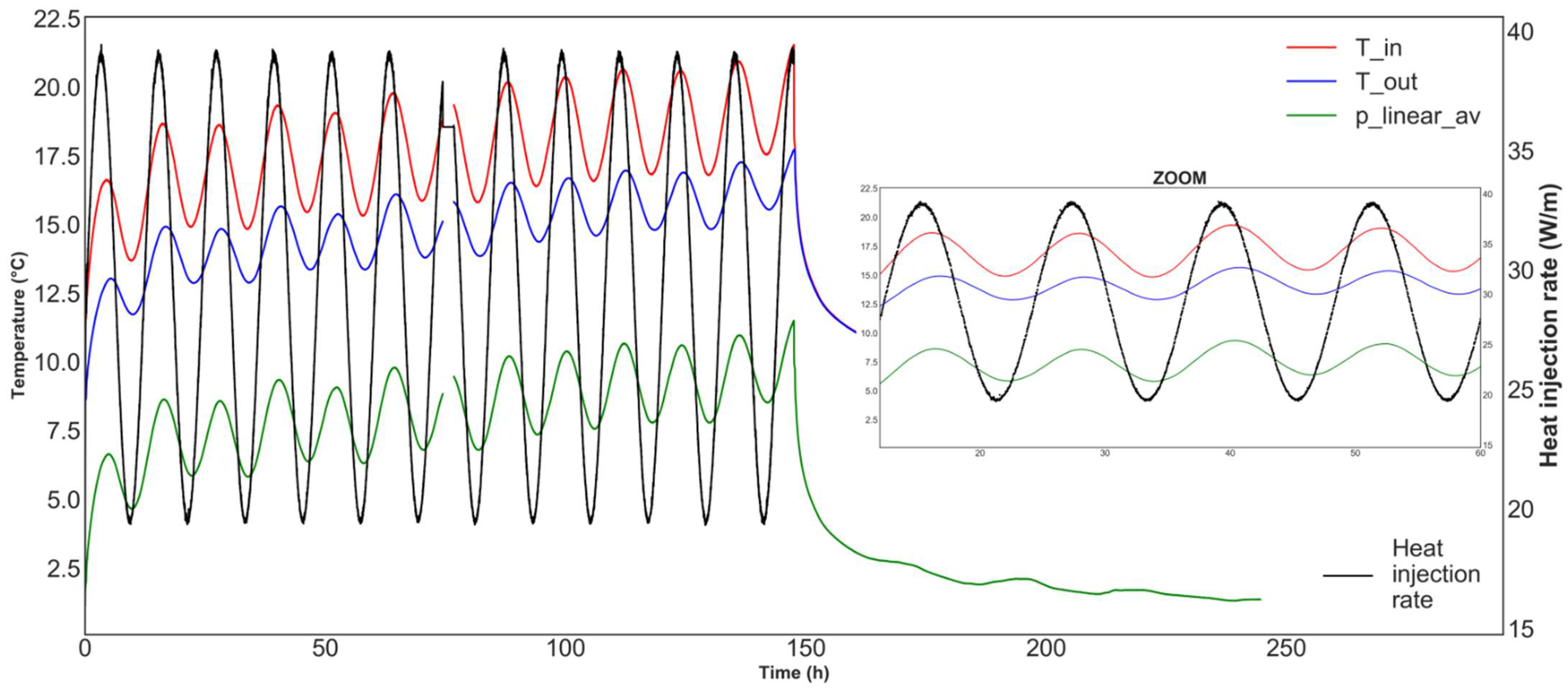
The OTRT was carried out for 147 h, with a period of oscillation of 12 h and an amplitude of 10 W m−1 (19 to 39 W m−1, Figure 9). The median power injected was 29.5 W m−1. The flow rate was constant at 0.385 ± 0.002 L s−1 (6.1 ± 0.03 GPM) throughout the entire test. Between 74 and 77 h, the monitoring system did not record any data, but the pump and heating element kept running as proved by back-up sensors along the circuit.
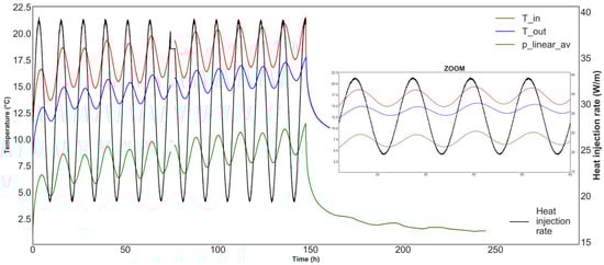
Figure 9.
Observed temperature during the OTRT carried out in the field. Inlet (red) and outlet (blue) temperature curves are in absolute values. p-linear average (green) curves show increments with respect to the initial temperature.
The p-linear average method (with p = −1) proposed by [40] was used to calculate the average BHE temperature in order to better represent the temperature profile along the BHE. p values of −2 (harmonic mean), −0.5 (geometric mean) and 1 (arithmetic mean) were also considered to evaluate its impact on the analysis of an OTRT. Maximum deviations were found between −1 and 1, in the order of 2.7 and 2.0% on and , respectively. The choice of using p = −1 rather than the conventional arithmetic mean (p = 1) reduces the HC by 0.18 and 0.16 MJ m−3 K−1 for and , respectively, which means 10% and 5% error in the final HC estimation. However, the TD results closer to the expected value were found with p = −1, and the uncertainty related to the chosen value of p is within the final range of HC, as explained in the discussion.
The analysis of the recovery period returns TC of 1.70 W m−1 K−1 (error 2.5%, Figure 10). By fixing the expected HC to 2.16 MJ m−3 K−1, the borehole thermal resistance estimation returns 0.075 m K W−1. This was computed by considering a test duration from 10 to 142 h, representing a total of 5.5 days. The first 10 h of the test were ignored to avoid disturbances and heat transfer within the BHE [2]. In addition, in an OTRT it is also crucial to respect the period of oscillation and pick the same phases at the beginning and at the end to avoid influencing the linear regression. Therefore, in this case an interval of 132 h (11 periods of oscillation) was used to analyze the OTRT results.
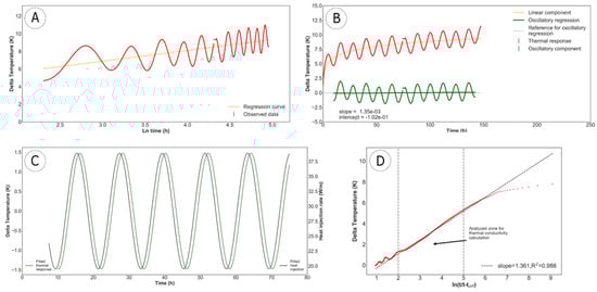
Figure 10.
Analysis of the OTRT carried out on the field: (A) evaluation of λheating and via the slope method; (B) split of the linear and oscillatory components; (C) comparison of the oscillatory heat injection and the oscillatory thermal response (the graph is cut at 75 h for simplicity); (D) analysis of the recovery period to estimate λcooling.
The oscillatory resistance is 0.15 m K W−1 and is 0.1 (Table 6). The TD estimation through Equations (5) and (6) returns values of 0.96 mm2 s−1 ( = 11 cm) and 0.48 mm2 s−1 ( = 8 cm), respectively (Table 7). As a result, TD and HC are significantly different when estimated from or . The TD and HC are closer to the expected subsurface values when evaluated via the oscillatory resistance, while they almost double when deduced from the phase shift (Table 8).
Table 6.
OTRT parameters inferred from the field test and related uncertainties δ (%).
Table 7.
Thermal diffusivity deduced from Equation (5) () and Equation (6) () and related uncertainties δ (%).
Table 8.
Heat capacity value deduced with TD from Table 7 and TC from the cooling period, and related uncertainties δ (%).
4. Discussion
The subsurface thermal properties evaluated from the heating cable TRT with temperature monitoring in the observation well are in agreement with literature values for the shales [8,9,10]. TC is slightly higher (10–12%) than that inferred by previous TRTs performed in the same BHE with water circulation (1.75 W m−1 K−1, [26]) and temperature logs (1.79 W m−1 K−1, [27]). This difference is most likely related to the shorter length investigated by this test (20 m), whereas previous tests surveyed the entire BHE length (154 m).
The OTRT performed in the field returned TD and HC in agreement with the expected values only when using the formulation function of the oscillatory resistance (, Equation (5)). On the other hand, the phase shift parameter appears highly affected by the BHE configuration, returning HC closer to the ones expected from the geothermal grout. This is in agreement with [17] and confirmed by the numerical simulations performed in this study.
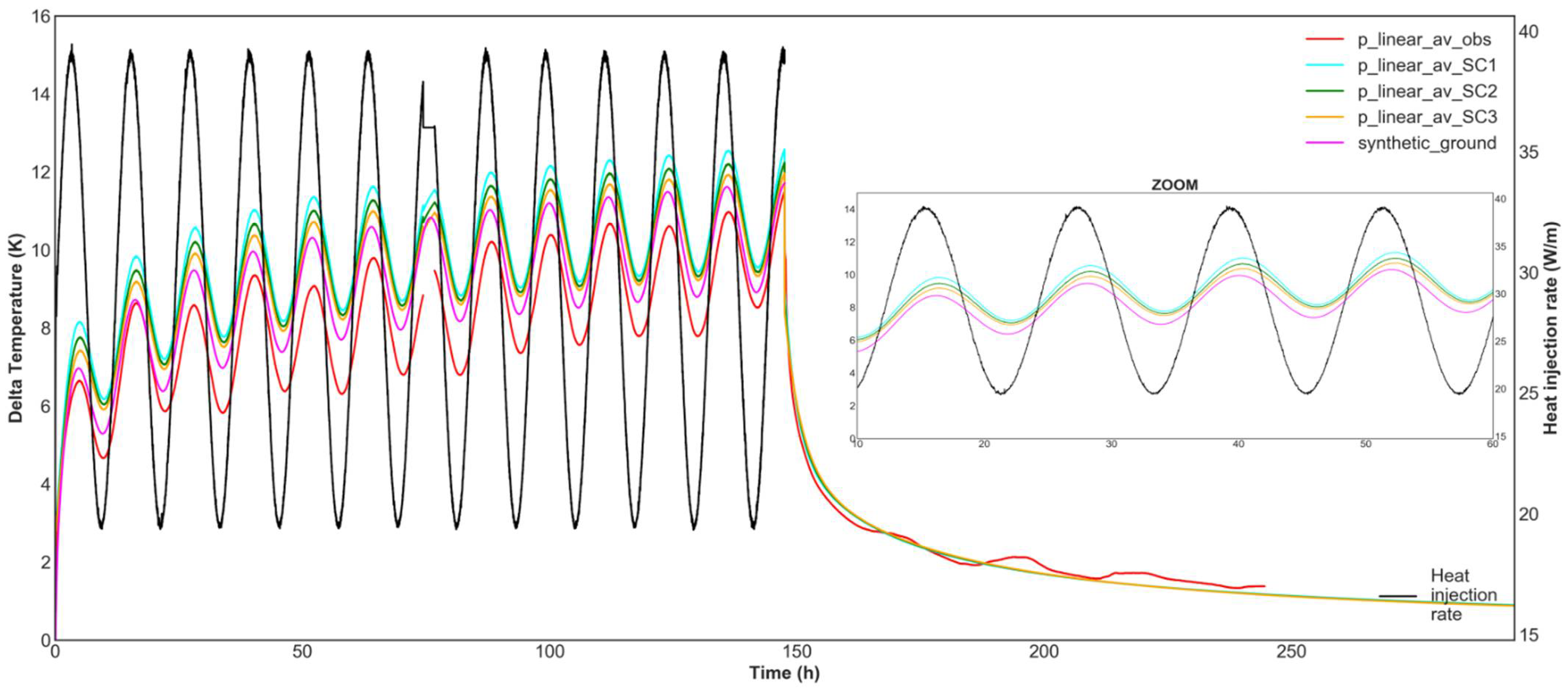
The oscillatory temperature response and associated parameters of two synthetic cases were calculated via the analytical expressions described in Equations (5) and (6) for comparison with the numerical and experimental results (Figure 11 and Table 9). The two cases were considered with: (1) thermal properties of the subsurface as estimated from the recovery period (TC 1.73 W m−1 K−1) and the observation well (TD of 0.8 mm2 s−1 and HC 2.16 MJ m−3 K−1); and (2) thermal properties of the backfilling BHE grout (TC 1.7 W m−1 K−1, TD of 0.44 mm2 s−1 and HC 3.9 MJ m−3 K−1). Compared to the subsurface synthetic case, experimental is 7% higher, while difference is >15% (Table 9). Compared to the grout synthetic case, experimental is higher by 17%, while shows maximum deviation of 5% (Table 9). This situation is comparable to the numerical simulations, with both and closer to the experimental results. In turn, we can say that in both the experimental OTRT and the numerical simulations the evaluation of the TD by means of the oscillatory resistance returns values close to the subsurface, while the phase shift appears highly affected by that of the backfilling material (Table 10). As aforementioned, HC results in the numerical simulations have a maximum deviation in absolute value of 20% for the first scenario, with the others being rather close (<9%) to the specified HC imposed as model input (Table 11). A fully transient numerical simulation would likely achieve closer values, but the results show that the analytical scheme to implement the BHE in FEFLOW (less computationally heavy, faster and easily applicable) is comparable to the field case. In general, numerical simulations indicate that the OTRT mainly underestimates the subsurface HC, with a maximum deviation of 20% (Table 11).
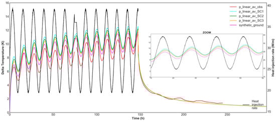
Figure 11.
Numerical results (SC1, SC2, SC3) compared to the observations (obs) and the analytical synthetic case based on subsurface input parameters.
Table 9.
Comparison of oscillation parameters obtained from the analysis of field tests and numerical simulations. The two reference cases calculated with ground and grout properties are also reported.
Table 10.
Comparison of thermal diffusivity obtained from the analysis of field tests and numerical simulations. TD of ground and grout are also reported.
Table 11.
Comparison of heat capacity obtained from the analysis of field tests and numerical simulations. HC of subsurface and grout are also reported.
The experimental OTRT demonstrated that the complex thermal response can be profitably split in a linear and an oscillatory component. Therefore, the linear component was used to estimate the TC and the borehole thermal resistance as commonly carried out with conventional TRT. The TC can be estimated via both the heating and the recovery period, but the latter is better in order to have the same accuracy as conventional TRT. This is particularly true if we consider different test duration and their impact on the evaluation of the borehole thermal resistance. Major changes were highlighted in the experimental observation. As clearly observed from Figure 9 and Figure 11, the temperature measurements recorded during the first 50–70 h of the test are less stable than those recorded after 70 h, with amplitude of the oscillation and slope of the linear component changing over time. The intercept of the linear regression is 4.60 K at 58 h ( 0.123), 4.46 K at 82 h ( 0.118), 3.82 K at 106 h ( 0.096) and 3.43 K at 130 h ( 0.083). However, this is not highlighted by the numerical simulations. So theoretically, the duration of the test does not influence the results. However, in practice, a longer test can help reduce the uncertainty on . When using the maximum possible duration of the test (142 h), the OTRT results underestimate by more than 15% the theoretical value calculated with the multipole method, as well as that previously found on the same 1-U BHE (0.088 m K W−1 [26,28]). This uncertainty is higher than what can be found via conventional TRT [39], which makes the OTRT hardly trustworthy at present for the estimation of the borehole thermal resistance. Further tests are therefore necessary to investigate this aspect in detail. On the contrary, no major changes due to the duration of the test were highlighted on the oscillatory parameters. Possible differences were found being within the uncertainty range reported in Table 9.
The parameters with the highest impact on the results of the OTRT analysis are the subsurface TC and the borehole thermal resistance. A 10% error in the estimation of the subsurface TC turns out in a 30% error estimation for the TD. The borehole thermal resistance, i.e., the BHE configuration (hole and pipe diameter, nature of the backfilling, etc.), impacts a major part of the OTRT response since a 12-h-period test has a depth of investigation of about 10 cm. Moreover, and TC of the backfill define the equivalent radius that has to be considered for the OTRT analysis (Equation (9)). From this study, it turns out that the linear regression coefficient of the oscillatory response cannot be accurate enough to provide a valid , which is highly dependent on the intercept of the linear fit. Therefore, as performed in the present study, a theoretical calculation is advisable. However, Table 12 shows that HC ranges on average from 1.65 to 2.2 MJ m−3 K−1 with varying from 0.086 to 0.1 m K W−1. This means that a 10% error estimation in returns a 24% variation in the final HC estimation.
In the light of these results and the previous experimental estimation of the borehole thermal resistance (0.09 m K W−1, [26,28]), the subsurface heat capacity at the study site is estimated to be in the range of 1.9 MJ m−3 K−1 ± 15%. Therefore, we can confirm that the heat capacity inferred by the OTRT is in agreement with the values expected after the heat diffusion analysis (2.1–2.2 MJ m−3 K−1, Section 3.1) if we consider three aspects: the numerical simulations showed that the proposed methodology tends to underestimate HC; the depth of the observation well OBS4 only allowed to investigate the shallowest 10 m of shales, while the BHE extends to 154 m below ground; and the depth of investigation of the OTRT is limited to the close vicinity of the BHE (12 cm radius). However, the final uncertainty range is similar to that found in the literature and, therefore, it would unlikely justify the execution of an OTRT. In the authors’ opinion, more work has to be carried out in order to improve the mathematical description of the OTRT and the analytical formulation to analyze field data. In particular, work should be focused on the understanding of the delayed found both in the field test and in the numerical simulations (0.1 vs. 0.085, see Table 9), as well as by [17]. It would be interesting to understand if this can be directly linked to the BHE configuration, and therefore to , such to be taken into account in the TD estimation via Equation (6). This would permit the reduction of the uncertainty found in this work, since Equation (5) is affected by the estimation of the TC. This aspect goes beyond the scope of the present contribution.
The limitations of this study mostly pertain to the benchmark analysis performed by means of the observation well. Its depth (shallow compared to the tested BHE) and inclination limited the heat diffusion analysis to the shallowest subsurface, half of it consisting of weathered shales. Moreover, there is no information about the exact inclination of the BHE, which was assumed to be vertical for simplicity. Future research projects that aim at comparing OTRT with observation wells must drill the wells one after the other, with the same drilling machine and operators. This will ensure to have, if not verticality in absolute terms, at least parallelism between them, such that the dual needle methodology used in laboratory analysis can easily be reproduced [41]. Finally, the volume investigated by the OTRT is limited to the close vicinity of the BHE, with a penetration depth of about 12 cm from the assumed linear source with equivalent radius of 2.2 cm.
5. Conclusions
Thermal response test (TRT) is the most common field method to infer the in-situ subsurface thermal conductivity (TC) in the scope of ground-coupled heat pump (GCHP) system design. Borehole thermal resistance can also be evaluated by means of TRT, which can help evaluate the performance of borehole heat exchangers (BHE). However, a TRT does not provide information about the subsurface heat capacity (HC), property which needs to be set via literature values. The aim of this research project was therefore to evaluate the effectiveness of an oscillatory thermal response test (OTRT) as a tool to infer the subsurface thermal diffusivity (TD; and hence the HC), in addition to TC and borehole thermal resistance, without the need of an observation well. To achieve this goal, numerical simulations and field testing were carried out. The main conclusions can be summarized as follows.
As oscillatory pumping test (OPT) allows the evaluation of the subsurface hydraulic diffusivity, OTRT can be carried out to estimate the thermal diffusivity. Even though having a penetration depth smaller than OPT, OTRT can induce an oscillatory thermal response in the same well/borehole whose smoothed amplitude and shifted phase contain information about the subsurface heat capacity. Dealing with abstraction and injection of heat from/to a BHE over a seasonal time scale, Eskilson [21] described the oscillatory thermal response induced by an oscillatory (sinusoidal) heat injection rate. He provided the expressions to infer the amplitude attenuation () and the phase shift (), parameters that are function of the subsurface TC and TD, and theoretically allow for an independent estimation of these thermal properties.
Field testing and numerical simulations performed in this study showed that the proposed methodology, based on the analytical approach described by Eskilson [21], can be used to infer the subsurface TD and HC without the need of a second well to record the heat diffusion. The OTRT was performed with a 12-h period in a grouted BHE made with a single U-pipe, having a depth of 154 m and a diameter of 0.114 m. Results show that the final HC estimated from a field test (1.9 MJ m−3 K−1 ± 15%) was likely underestimated. This fact was also confirmed by numerical simulations of OTRT. The result is affected by a range of variation similar to what can be found in the literature, therefore making the OTRT unlikely applicable at present. Higher-period tests (12–24 h) can be carried out within the conventional duration of TRTs. This would increase the penetration depth of the oscillatory signal, but the accuracy of the result is expected to decrease. The parameters having the greatest impact on the results are the subsurface TC and the borehole thermal resistance. While the former can be assessed with an OTRT, the latter cannot be defined with valid accuracy. This has direct effects on the calculation of the equivalent radius, i.e., the distance at which the oscillatory parameters and are calculated. Conversely to the Eskilson’s theory, can be used to evaluate the subsurface heat capacity, while is affected by a delay of 0.02. This outcome was found for both the experimental and numerical results, and it appears to be due to heat storage in the borehole, which is not considered in the borehole thermal resistance calculation.
The OTRT methodology proposed in this contribution can concurrently allow evaluating the subsurface TC with similar accuracy compared to conventional TRTs (<3%, [2,7] and references therein). However, it is suggested to use the recovery period in order to avoid the influence of the borehole thermal resistance. The latter was also evaluated from the field test, but the accuracy of this estimation was not entirely satisfactory. Further investigation on this matter is therefore needed.
Finally, OTRT seems a promising tool to evaluate the HC, but more field testing (different geological settings, BHE configurations, temperature sensors, flow meters, etc.) and mathematical interpretation of the oscillatory response are necessary to better isolate the subsurface contribution from the complex response in the BHE. To this regard, future activities will focus on the quantification of the borehole thermal resistance within the signal’s phase shift to allow for an independent estimation of the TD by means of . As a further step, OTRT could be carried out with different periods of oscillation and the subsurface response would then be analyzed in the frequency domain as already made by [17] and applied to harmonic well testing in the petroleum industry by [42]. It is in the authors’ opinion that the accuracy of HC estimate should be <10% for the OTRT to be commonly implemented in the scope of GCHP system design.
Author Contributions
Conceptualization, J.R., N.G. and L.L.; methodology, N.G., J.R. and L.L.; software, N.G.; validation, N.G., L.L. and J.R.; formal analysis, N.G.; investigation, N.G.; resources, J.R. and L.L.; data curation, N.G., J.R. and L.L.; writing—original draft preparation, N.G.; writing—review and editing, N.G., J.R. and L.L.; visualization, N.G.; supervision, J.R. and N.G.; project administration, J.R. and L.L.; funding acquisition, J.R. and L.L. All authors have read and agreed to the published version of the manuscript.
Funding
This research was funded by the Natural Sciences and Engineering Research Council (NSERC) of Canada through an Idea to Innovation grant awarded to J.R. and L.L., and an exploration grant from the New Frontiers in Research Fund awarded to J.R. The APC was funded by the exploration grant from the New Frontiers in Research Fund awarded to J.R.
Institutional Review Board Statement
Not applicable.
Informed Consent Statement
Not applicable.
Data Availability Statement
The data presented in this study as well as the Python scripts for analysis are available on request to the corresponding author.
Acknowledgments
Special thanks to Energie Stat (http://www.energie-stat.com/, accessed on 9 September 2021) for carrying out two OTRTs and giving us proper results; we highly appreciate their effort for the success of this project. Additional thanks go to Jean-Marc Ballard (INRS) for the drilling of the observation wells 4 and 5. In particular, OBS4 was quite challenging due to the request of it being parallel to the nearby BHE. We highly appreciate Jean-Marc’s involvement in the project. Éric Allard by Semm Logging (http://www.semmlogging.com/, accessed on 9 September 2021) is also thanked for the well inclination analysis performed with Gyromaster. Final acknowledgements go to the three reviewers that helped to improve the clarity of this manuscript.
Conflicts of Interest
N.G. is vice-president and co-founder of Géotherma solutions inc (https://geotherma.ca/, accessed on 9 September 2021). L.L. and J.R. declare no conflict of interest.
Nomenclature
| amplitude of the thermal response [K] | |
| amplitude of the heat injection [W m−1] | |
| depth of penetration [m] | |
| deviation from the expected value [%] | |
| borehole depth [m] | |
| oscillation period [s] or [h] | |
| heat injection/extraction rate [W m−1] | |
| distance [m] | |
| borehole radius [m] | |
| equivalent borehole radius [m] | |
| dimensionless factor [-] | |
| internal borehole thermal resistance [m K W−1] | |
| borehole thermal resistance [m K W−1] | |
| internal borehole thermal resistance including pipe resistance [m K W−1] | |
| borehole thermal resistance including pipe resistance [m K W−1] | |
| equivalent borehole thermal resistance including pipe resistance [m K W−1] | |
| grout-to-grout resistance [m K W−1] | |
| oscillatory resistance [m K W−1] | |
| time [s] | |
| temperature [K] or [°C] | |
| shank spacing [m] | |
| Greek symbols | |
| thermal diffusivity [m2 s−1] | |
| Euler-Mascheroni constant 0.5772156649 [-] | |
| δ | relative error (uncertainty) of the estimation [%] |
| thermal conductivity of the subsurface [W m−1 K−1] | |
| thermal conductivity of the grout [W m−1 K−1] | |
| phase shift [-] | |
| Abbreviations | |
| 1-U | single U |
| BHE | borehole heat exchanger |
| GW | groundwater |
| GCHP | ground-coupled heat pump |
| HC | heat capacity |
| NNW | north/north-west |
| NW | north-west |
| OBS | observation well |
| OPT | oscillatory pumping test |
| OTRT | oscillatory thermal response test |
| SDR | standard dimension ratio |
| TC | thermal conductivity |
| TD | thermal diffusivity |
| TRCM | thermal resistance and capacity model |
| TRT | thermal response test |
| UTES | underground thermal energy storage |
Appendix A. Analytical Validation of the Proposed Methodology
The simplified analytical approach proposed by Eskilson (Equations (5)–(8)) and used in the above methodology was verified with analysis of oscillating temperature responses computed with fixed subsurface thermal properties (TC 1.7 W m−1 K−1, TD of 0.7 mm2 s−1 and HC 2.43 MJ m−3 K−1) and different BHE diameter (4.5 and 6 inches). A sinusoidal heat injection with amplitude of 10 W m−1 and offset of 30 W m−1 was used in the calculation of the oscillating temperature response. Target periods of oscillations were set to 12 and 24 h, so that the OTRT can last a maximum of 72 h. The equivalent borehole radius was calculated with grout TC equal to 1.7 W m−1 K−1 and equal to 0.09 m K W−1, resulting in 0.022 and 0.029 m for a 4.5-inch (0.114 m) and a 6-inch (0.152 m) BHE, respectively.
Results of this validation indicate a factor ranging from 0.2 to 0.4, and a depth of investigation varying from 0.10 to 0.15 m for the four scenarios considered (Table A1). The proposed methodology returns thermal diffusivity and heat capacity with absolute deviation from the expected value (D [%]) of 1–2% considering 12-h periods (Table A2 and Table A3). A more important deviation (6–7% in absolute value) is obtained when using 24-h periods, with a maximum of 15% when the analysis is made via Equation (6). In mathematical terms, Equations (5) and (6) can be independently used to assess the subsurface thermal properties because is a function of TD and TC, whereas is only function of TD. However, this validation shows that the two equations have different sensitivities to subsurface TD. The expression function of the oscillatory resistance (, Equation (5)) is generally more accurate.
Table A1.
Oscillatory parameters inferred from the validation of the analytical procedure.
Table A1.
Oscillatory parameters inferred from the validation of the analytical procedure.
| (-) | (-) | |||
|---|---|---|---|---|
| 4.5-inch/P 12 h | 0.140 | 0.089 | 0.316 | 0.097 |
| 6-inch/P 12 h | 0.118 | 0.106 | 0.420 | 0.099 |
| 4.5-inch/P 24 h | 0.165 | 0.071 | 0.230 | 0.141 |
| 6-inch/P 24 h | 0.142 | 0.081 | 0.305 | 0.149 |
Table A2.
Thermal property estimation for validation of the analytical procedure.
Table A2.
Thermal property estimation for validation of the analytical procedure.
| 4.5-inch/P 12 h | 0.694 | 2.451 | 0.684 | 2.485 |
| 6-inch/P 12 h | 0.696 | 2.443 | 0.715 | 2.378 |
| 4.5-inch/P 24 h | 0.650 | 2.614 | 0.722 | 2.356 |
| 6-inch/P 24 h | 0.659 | 2.581 | 0.805 | 2.113 |
Table A3.
Thermal diffusivity and heat capacity deviation D (%) from the expected 0.70 mm2 s−1 and 2.43 MJ m−3 K−1, respectively.
Table A3.
Thermal diffusivity and heat capacity deviation D (%) from the expected 0.70 mm2 s−1 and 2.43 MJ m−3 K−1, respectively.
| 4.5-inch/P 12 h | −0.9 | 0.9 | −2.3 | 2.3 |
| 6-inch/P 12 h | −0.6 | 0.6 | 2.1 | −2.1 |
| 4.5-inch/P 24 h | −7.1 | 7.6 | 3.1 | −3.0 |
| 6-inch/P 24 h | −5.9 | 6.3 | 15.0 | −13.0 |
This difference in the sensitivity can be explained by the first order approximation of the Kelvin function provided by [21] to obtain Equations (5) and (6). A comparison of the exact solution to the first and second-order approximations is reported in Figure A1 and Figure A2 for the oscillatory resistance and phase shift as a function of , respectively. The first-order approximation proposed by Eskilson deviates from the exact solution with increasing values of for both and . However, the deviation for starts already at , thus affecting the results with higher inconsistency as reported in Table A3. It is important to say that the deviations from the expected value of thermal diffusivity are not related to the use of Eskilson’s simplified analytical expressions in place of the exact solution. In the study reported in the paper, with equal to 0.298, the thermal diffusivity difference between the first-order approximation and the exact solution for is 1.5%, i.e., within the final uncertainty range discussed in the paper. The difference for is much higher (48%), but even the exact solution is 70% lower than the expected value of thermal diffusivity. The inconsistencies highlighted in the present study are related to the complex relationship between , and the temperatures at and , and not due to the use of approximate vs. exact solutions.
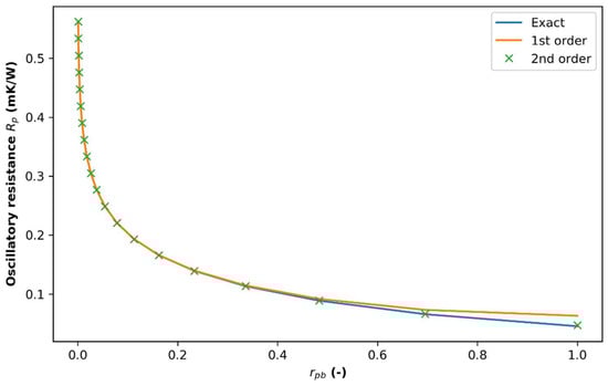
Figure A1.
Comparison of the Taylor series expansion of the Kelvin funcion (blue line) with first (orange line) and second-order (green stars) approximations for the oscillatory resistance as a function of . Equation (5) reported in the manuscript has been obtained by Eskilson with a first-order approximation.
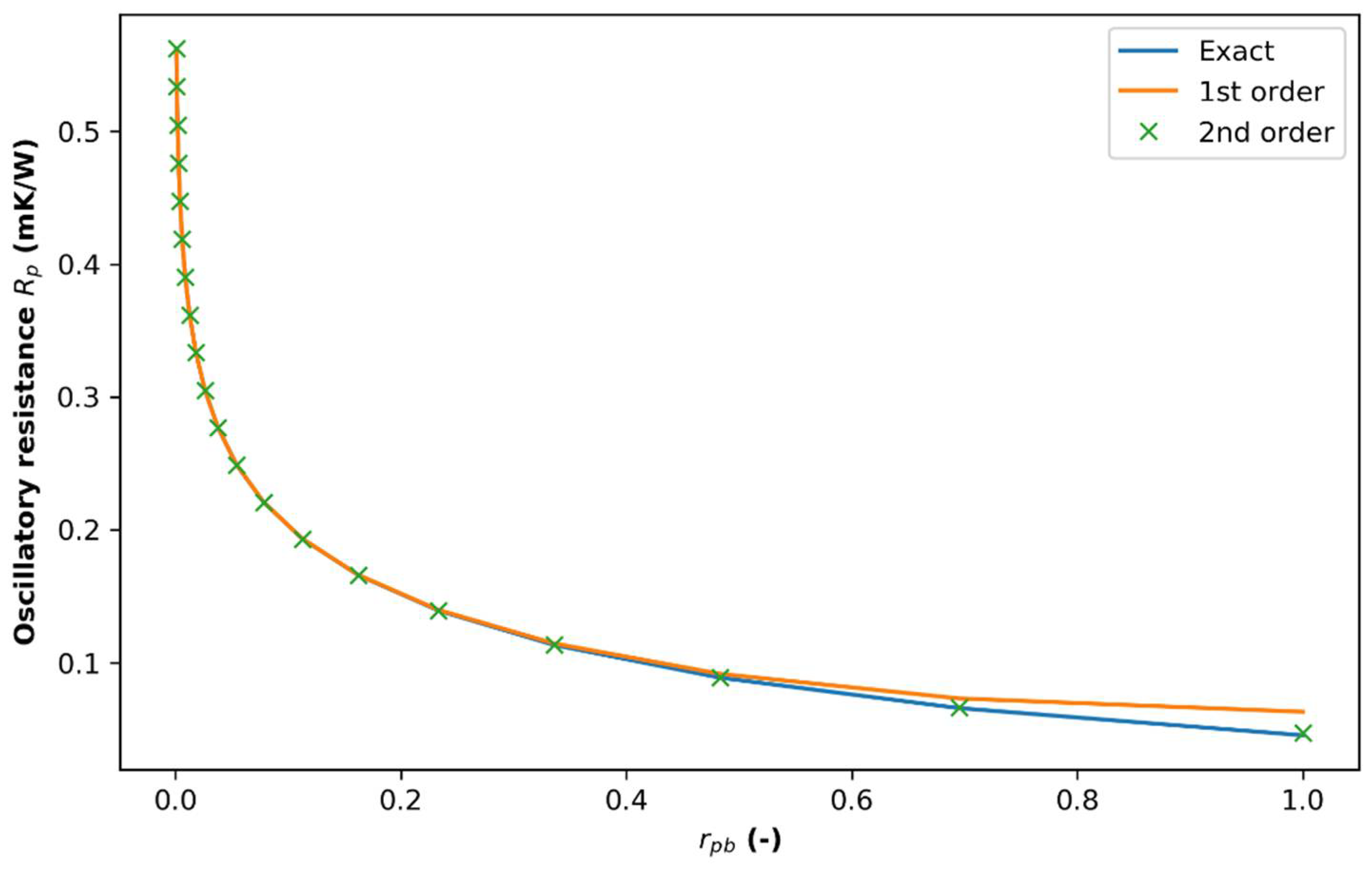
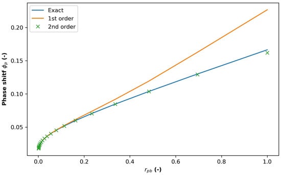
Figure A2.
Comparison of the Taylor series expansion of the Kelvin funcion (blue line) with first-order (orange line) and second-order (green stars) approximations for the phase shift as a function of . Equation (6) reported in the manuscript has been obtained by Eskilson with a first-order approximation.

Finally, it was found that the Eskilson approximation (first order) provides valid results until for when considering an equivalent BHE radius. Periods of oscillations in the order of 10–12 h for 4.5-inch BHE (0.114 m) and of 18–20 h for 6-inch BHE (0.152 m) are expected to provide valid results with the proposed methodology. This allows for carrying out OTRTs with duration similar to conventional TRTs (i.e., 48–72 h). However, the subsurface volume investigated is limited to the close vicinity of the BHE, with equal to 10–13 cm.
Appendix B. Assumptions and Simplifications
The use of an equivalent BHE radius (Equation (9)) is a simplification of the BHE geometry to a 1-D model. This has proved to be necessary because the Eskilson’s analytical solution refers to the borehole wall temperature (Equation (2)), while in the present study the fluid temperature is analyzed. Equation (9) can easily be derived by the well-know expression of the thermal resistance of a single pipe due to heat conduction ([37,38] and references therein), and where the outside and internal pipe radius are replaced by and , respectively:
Clearly, a 1-D model that simplifies the BHE to a heated line involves significant assumptions that, for instance, do not take into account the thermal short circuiting between the 2 (or 4) pipes of the BHE, e.g., [42,43,44,45]. As these authors highlighted, 1-D is inadequate when simulating the real operation of BHE fields, but for a TRT of short duration, where the purpose is to infer the underground thermal conductivity and the borehole thermal resistance, the simplification holds. Indeed, the infinite or finite line source models are still the conventional way to interpret TRT results since quasi steady-state conditions are reached inside the BHE after 10–15 h from the beginning of the test. In the present study, it has been found that the OTRT also reaches steady-state inside the BHE after 10–15 h. Therefore, it is in the authors’ opinion that a simplified 1-D model can be considered appropriate.
References
- Kavanaugh, S.P. Investigation of Methods for Determining Soil Formation Thermal Characteristics from Short Term Field Tests; ASHRAE: Atlanta, GA, USA, 2001. [Google Scholar]
- Spitler, J.D.; Gehlin, S.E.A. Thermal response testing for ground source heat pump systems—An historical review. Renew. Sustain. Energy Rev. 2015, 50, 1125–1137. [Google Scholar] [CrossRef]
- Raymond, J.; Lamarche, L.; Malo, M. Field demonstration of a first thermal response test with a low power source. Appl. Energy 2015, 147, 30–39. [Google Scholar] [CrossRef]
- Márquez, M.I.V.; Raymond, J.; Blessent, D.; Philippe, M.; Simon, N.; Bour, O.; Lamarche, L. Distributed thermal response tests using a heating cable and fiber optic temperature sensing. Energies 2018, 11, 3059. [Google Scholar] [CrossRef] [Green Version]
- Zhang, B.; Gu, K.; Shi, B.; Liu, C.; Bayer, P.; Wei, G.; Gong, X.; Yang, L. Actively heated fiber optics based thermal response test: A field demonstration. Renew. Sustain. Energy Rev. 2020, 134, 110336. [Google Scholar] [CrossRef]
- Kurevija, T.; Macenić, M.; Strpić, K. Steady-State Heat Rejection Rates for a Coaxial Borehole Heat Exchanger During Passive and Active Cooling Determined With the Novel Step Thermal Response Test Method. Mining-Geol.-Pet. Eng. Bull. 2018, 33, 61–71. [Google Scholar] [CrossRef] [Green Version]
- Aydin, M.; Onur, M.; Sisman, A. A new method for analysis of constant-temperature thermal response tests. Geothermics 2019, 78, 1–8. [Google Scholar] [CrossRef]
- Dalla Santa, G.; Galgaro, A.; Sassi, R.; Cultrera, M.; Scotton, P.; Mueller, J.; Bertermann, D.; Mendrinos, D.; Pasquali, R.; Perego, R.; et al. An updated ground thermal properties database for GSHP applications. Geothermics 2020, 85, 101758. [Google Scholar] [CrossRef]
- VDI Thermal Use of the Underground 2010. Available online: https://www.vdi.de/richtlinien/details/vdi-4640-blatt-1-thermal-use-of-the-underground-fundamentals-approvals-environmental-aspects (accessed on 9 September 2021).
- Kavanaugh, S.; Rafferty, K. Geothermal Heating and Cooling: Design of Ground-Source Heat Pump Systems; ASHRAE: Atlanta, GA, USA, 2014; ISBN 9781936504855. [Google Scholar]
- Skarphagen, H.; Banks, D.; Frengstad, B.S.; Gether, H. Design Considerations for Borehole Thermal Energy Storage (BTES): A Review with Emphasis on Convective Heat Transfer. Geofluids 2019, 2019, 4961781. [Google Scholar] [CrossRef]
- Giordano, N.; Raymond, J. Alternative and sustainable heat production for drinking water needs in a subarctic climate (Nunavik, Canada): Borehole thermal energy storage to reduce fossil fuel dependency in off-grid communities. Appl. Energy 2019, 252, 113463. [Google Scholar] [CrossRef]
- Raymond, J.; Comeau, F.; Malo, M.; Blessent, D.; Sánchez López, J.I. The Geothermal Open Laboratory: A free space to measure thermal and hydraulic properties of geological materials. In Proceedings of the IGCP636 Annual Meeting, Santiago, Chile, 21 November 2017; p. 4. [Google Scholar]
- Cardiff, M.; Bakhos, T.; Kitanidis, P.K.; Barrash, W. Aquifer heterogeneity characterization with oscillatory pumping: Sensitivity analysis and imaging potential. Water Resour. Res. 2013, 49, 5395–5410. [Google Scholar] [CrossRef] [Green Version]
- Guiltinan, E.; Becker, M.W. Measuring well hydraulic connectivity in fractured bedrock using periodic slug tests. J. Hydrol. 2015, 521, 100–107. [Google Scholar] [CrossRef] [Green Version]
- Raymond, J.; Lamarche, L. Simulation of thermal response tests in a layered subsurface. Appl. Energy 2013, 109, 293–301. [Google Scholar] [CrossRef]
- Oberdorfer, P. Heat Transport. Phenomena in Shallow Geothermal Boreholes—Development of a Numerical Model. and a Novel Extension for the Thermal Response Test. Method by Applying Oscillating Excitations; Georg-August University of Gottingen: Göttingen, Germany, 2014. [Google Scholar]
- Carslaw, H.S.; Jaeger, J.C. Conduction of Heat in Solids; Oxford University Press: Oxford, UK, 1947. [Google Scholar]
- Philippe, M.; Bernier, M.; Marchio, D. Validity ranges of three analytical solutions to heat transfer in the vicinity of single boreholes. Geothermics 2009, 38, 407–413. [Google Scholar] [CrossRef]
- Casasso, A.; Ferrantello, N.; Pescarmona, S.; Bianco, C.; Sethi, R. Can borehole heat exchangers trigger cross-contamination between aquifers? Water 2020, 12, 1174. [Google Scholar] [CrossRef]
- Eskilson, P. Thermal Analysis of Heat Extraction Boreholes; University of Lund: Lund, Sweden, 1987. [Google Scholar]
- Raymond, J.; Therrien, R.; Gosselin, L. Borehole temperature evolution during thermal response tests. Geothermics 2011, 40, 69–78. [Google Scholar] [CrossRef]
- Aydin, M.; Gultekin, A.; Sisman, A. The effects of test temperature and duration on the results of constant temperature thermal response test. In Proceedings of the 12th IEA Heat Pump Conference, Rotterdam, NL, USA, 29 May 2017; p. 9. [Google Scholar]
- Globensky, Y. Géologie des Basses Terres du Saint-Laurent; Bibliothèque Nationale du Québec: Quebec City, QC, Canada, 1987. [Google Scholar]
- Ballard, J.M.; Koubikana Pambou, C.H.; Raymond, J. Évaluation de la Performance D’un Forage Géothermique de Conception Améliorée; Institut National de la Recherche Scientifique: Quebec City, QC, Canada, 2019. [Google Scholar]
- Ballard, J.M.; Koubikana Pambou, C.H.; Raymond, J. Développement des Tests de Réponse Thermique Automatisés et Vérification de la Performance d’un Forage Géothermique d’un Diamètre de 4,5 po; Institut national de la Recherche Scientifique: Québec City, QC, Canada, 2016. [Google Scholar]
- Koubikana Pambou, C.H.; Raymond, J.; Lamarche, L. Improving thermal response tests with wireline temperature logs to evaluate ground thermal conductivity profiles and groundwater fluxes. Heat Mass Transf. Stoffuebertragung 2019, 55, 1829–1843. [Google Scholar] [CrossRef]
- Raymond, J.; Ballard, J.; Pambou Koubikana, C.H.; Kwemo, P. Field assessment of a ground heat exchanger performance with a reduced borehole diameter. In Proceedings of the 70th Canadian Geotechnical Conference and the 12th Joint CGS/IAH-CNC Groundwater Conference, Ottawa, ON, Canada, 1–4 October 2017; p. 6. [Google Scholar]
- Diersch, H.-J.G. FEFLOW Finite Element Modeling of Flow, Mass and Heat Transport in Porous and Fractured Media; Springer: Berlin/Heidelberg, Germany, 2014; ISBN 9783642387388. [Google Scholar]
- Diersch, H.-J.G.; Bauer, D.; Heidemann, W.; Ruhaak, W.; Schatzl, P. Finite element modeling of borehole heat exchanger systems Part 2. Numerical simulation. Comput. Geosci. 2011, 37, 1136–1147. [Google Scholar] [CrossRef]
- Eskilson, P.; Claesson, J. Simulation model for thermally interacting heat extraction boreholes. Numer. Heat Transf. 1988, 13, 149–165. [Google Scholar] [CrossRef]
- Al-Khoury, R.; Bonnier, P.G.; Brinkgreve, R.B.J. Efficient finite element formulation for geothermal heating systems. Part I: Steady state. Int. J. Numer. Methods Eng. 2005, 63, 988–1013. [Google Scholar] [CrossRef]
- Diersch, H.-J.G.; Bauer, D.; Heidemann, W.; Ruhaak, W.; Schatzl, P. Finite element modeling of borehole heat exchanger systems Part 1. Fundamentals. Comput. Geosci. 2011, 37, 1122–1135. [Google Scholar] [CrossRef]
- Bauer, D.; Heidemann, W.; Müller-Steinhagen, H.; Diersch, H.-J.G. Thermal resistance and capacity models for borehole heat exchangers. Int. J. Energy Res. 2011, 35, 312–320. [Google Scholar] [CrossRef]
- Bennet, J.; Claesson, J.; Hellström, G. Multipole Method to Compute the Conductive Heat Flows to and between Pipes in a Composite Cylinder. Ph.D. Thesis, Lund University, Lund, Sweden, 1987. [Google Scholar]
- Claesson, J.; Hellström, G. Multipole method to calculate borehole thermal resistances in a borehole heat exchanger. HVAC&R Res. 2011, 17, 895–911. [Google Scholar] [CrossRef]
- Lamarche, L.; Kajl, S.; Beauchamp, B. A review of methods to evaluate borehole thermal resistances in geothermal heat-pump systems. Geothermics 2010, 39, 187–200. [Google Scholar] [CrossRef]
- Hellström, G. Ground Heat Storage, Thermal Analyses of Duct Storage Systems, Part I: Theory. Ph.D. Thesis, University of Lund, Lund, Sweden, 1991. [Google Scholar]
- Witte, H.J.L. Error analysis of thermal response tests. Appl. Energy 2013, 109, 302–311. [Google Scholar] [CrossRef]
- Marcotte, D.; Pasquier, P. On the estimation of thermal resistance in borehole thermal conductivity test. Renew. Energy 2008, 33, 2407–2415. [Google Scholar] [CrossRef]
- Fokker, P.A.; Salina Borello, E.; Verga, F.; Viberti, D. Harmonic pulse testing for well performance monitoring. J. Pet. Sci. Eng. 2018, 162, 446–459. [Google Scholar] [CrossRef]
- Yang, H.; Cui, P.; Fang, Z. Vertical-borehole ground-coupled heat pumps: A review of models and systems. Appl. Energy 2010, 87, 16–27. [Google Scholar] [CrossRef]
- Zeng, H.; Diao, N.; Fang, Z. Efficiency of Vertical Geothermal Heat Exchangers in the Ground Source Heat Pump System. J. Therm. Sci. 2003, 12, 77–81. [Google Scholar] [CrossRef]
- Yavuzturk, C.; Spitler, J.D.; Rees, S.J. A Transient two-dimensional finite volume model for the simulation of vertical U-tube ground heat exchangers. ASHRAE Trans. 1999, 105, 465–474. [Google Scholar]
- Gu, Y.; O’Neal, D.L. Development of an equivalent diameter expression for vertical U-tubes used in ground-coupled heat pumps. ASHRAE Trans. 1998, 104, 347–355. [Google Scholar]


Publisher’s Note: MDPI stays neutral with regard to jurisdictional claims in published maps and institutional affiliations. |
© 2021 by the authors. Licensee MDPI, Basel, Switzerland. This article is an open access article distributed under the terms and conditions of the Creative Commons Attribution (CC BY) license (https://creativecommons.org/licenses/by/4.0/).