Article

The Problem of Non-Typical Objects in the Multidimensional Comparative Analysis of the Level of Renewable Energy Development

Department of Decision Support Methods and Cognitive Neuroscience, University of Szczecin, 71-004 Szczecin, Poland
*
Author to whom correspondence should be addressed.
Energies 2021, 14(18), 5803; https://doi.org/10.3390/en14185803
Submission received: 11 August 2021 / Revised: 7 September 2021 / Accepted: 8 September 2021 / Published: 14 September 2021
(This article belongs to the Special Issue Energy Decision Making: Problems, Methods, and Tools)

Abstract

:
The development of energy from renewable sources is one of the most important aspects of today’s energy industry. The level of this development (production of green energy) is determined by the use of a variety of methods, e.g., the methods of multicriteria and multivariate analysis. The effectiveness of these methods is affected by many factors, and one of them is the appearance of non-typical objects (outliers). This paper investigates the effectiveness of selected methods (TOPSIS, VIKOR, VMCM) in terms of computational robustness to outlier objects. The most effective method in this respect (VMCM) is then applied to study the level of development of renewable energy sources in European countries. The presented research provides the opportunity to carry out a dynamic analysis (for selected base years) of the level of energy generation from diverse renewable sources in reference to the adopted patterns and anti-patterns (European countries). The obtained results are discussed, thus confirming the effectiveness of the proposed methodological approach.

1. Introduction

For years, energy has been a key resource in human development. Its sustainable development includes the use of available energy resources so that this development can be long-lasting and environmentally friendly. Energy development is intertwined with other dimensions of sustainable development, e.g., with social, economic and environmental dimensions. Economic growth determines the increase in energy demand, and this in turn is connected with environmental impacts, e.g., directly aggravating global climate change (global warming) [1]. Therefore, the goal of sustainable energy policies is to achieve a satisfactory level of energy availability while maintaining appropriate levels of economic, social and environmental systems. Various international initiatives aim to serve this purpose. One of them is the 2030 Agenda for Sustainable Development. It is a document (adopted by UN countries), which is a comprehensive development plan for the world with a perspective of reaching its goals by 2030. [2]. One of the seventeen Sustainable Development Goals (SDGs) addresses the issue of energy. This goal (SDG 7) is aimed at ensuring that all people have access to affordable, reliable, sustainable and modern energy. One of the important actions embedded in this goal is increasing the share of renewable energy (RE) in the global energy mix [3]. In 2020, the leading countries in terms of renewable energy generated were China (895 GW), USA (292 GW) and Brazil (150 GW). In the same period, the biggest consumers of renewable energy were, respectively, China, the USA and Germany [4].
The energy transition towards renewable energy is evident in many countries around the world. In Europe, it is the European Union (EU), or rather its relevant institutions, that is responsible for such energy transformation. The adopted renewable energy policy system includes, among others things, strategies (short-, medium- and long-term), support mechanisms and development standards [5]. The essential legal basis for the EU energy policy comprises the EU Emissions Trading Scheme (EU ETS) [6], as well as a number of directives, such as the Directive on the promotion of the use of energy from renewable sources (RED II, 2018) [7], the Energy Efficiency Directive (2018) [8] or the Directive on common rules for the internal market in electricity (2019) [9]. Adopted in 2019, the European Green Deal for the European Union assumes that net zero greenhouse gas emissions will have been achieved by 2050 [10,11,12]. According to the forecast by the International Renewable Energy Agency (IRENA), the share of renewable energy could account for more than 33% of EU energy generation in 2030 and as much as 94% in 2050 [13,14]. Brazil, being at the forefront of countries using renewable energy (mainly biomass), is constantly developing and promoting the development of hydropower and wind energy [5]. In the adopted 10-year Energy Development Plan 2029, Brazil has decided to increase the energy efficiency of the Brazilian Power System (BPS) with emphasis put on the transition to energy sources ensuring lower greenhouse gas emissions [15,16]. The main development directions concern hydropower potential and wind power [17]. China has made a major contribution to energy transition in recent years. It is implementing structural reforms in the context of energy supply, its efficient use and the growth of renewable energy [18]. It has committed to achieving peak emissions by 2030 and emissions neutrality by 2060 [19]. In the US, renewable energy is the fastest-growing energy source. In 2020, it was also the only source of energy consumption to increase from 2019 [20]. Renewable energy is also expected to be the most rapidly growing source of electricity generated in the US by 2050. This growth is most evident in biofuels, solar and wind [21,22]. The American energy policy involves government actions at multiple administrative levels addressing the production, distribution, and consumption of various energy sources (including renewable energy). It is conducted at the local, state and federal levels. The EPA (Environmental Protection Agency) sets and enforces legal standards in consultation with state, local and tribal governments.
Despite the obvious advantages of renewable energy (e.g., reducing fossil fuel consumption, decreasing CO2 emissions) [23,24,25,26], its development faces a number of barriers. Some of them are related to the specifics of the region (e.g., ecological issues, availability of land), some of the limitations come from technology (e.g., lack of grid connections) and others are related to economic issues (e.g., lack of financial subsidies, credits) and even political issues (e.g., lack of RES policy) [27,28,29,30,31].
The development of renewable energy is an important part of the energy policy of almost every country. Various national and international institutions are being established to develop legal solutions favoring the development of renewable energy and to monitor their implementation [32]. Many other institutions (e.g., scientific, commercial) also conduct research examining the investments in RE or the degree of its development. Different methodological approaches are used for this, and different models are built [33]. Some of them are based on multicriteria decision-making (MCDM)/multicriteria decision analysis (MCDA) or multidimensional comparative analysis (MCA). Examples of the application of multicriteria and multidimensional analysis methods in the context of renewable energy decisions are numerous in the world literature. For instance, as regards its planning (i.e., selecting the RE sources), there are studies using AHP [34,35,36], ANP [37,38], ELECTREE [39], PROMETHEE [40], TOPSIS [41,42,43,44], VIKOR [45] and other methods [46,47,48]. The same methods find applications in renewable energy source site selection [36,37,38,39,40,41,42,43,44,45,46,47,48] as well as in sustainable energy planning assessment [49,50,51,52,53,54,55,56,57,58,59]. They are also employed in decision-making processes related to technology selection (materials, components, etc.) [60,61,62,63,64,65,66,67,68,69]. To assess the level of renewable energy development, researchers often use synthetic measures based on different sets of indicators) and methods such as TOPSIS, PCA, etc. in addition to econometric analyses [70,71,72,73]. The analyses using MCDM/MCDA and MCA methods are complex because they involve a multidimensional space of various indicators, targets and constraints. Different methods may produce different results, and the choice of a particular method should be tailored to the specific problem [74,75]. When applying a method, one should, among other things, know its limitations. One such limitation for benchmark methods (e.g., TOPSIS, VIKOR) may be the distribution of data in multidimensional space. In situations where some data (objects) are significantly distant from the adopted pattern, they may significantly affect the final results of the analysis. These are the so-called non-typical objects.
The purpose of this paper is to show the problem of non-typical objects in the selected methods of multicriteria/multidimensional analysis (TOPSIS, VIKOR) and then to propose a methodical approach (the original VMCM method) to solve this problem in the context of research into the level of renewable energy generation in European countries. The choice of these methods, TOPSIS, VIKOR and VMCM, was dictated by their similar properties and the fact that they can be used to analyze large data sets with minimal involvement of the decision maker. They are methods on the borderline between multivariate comparative analysis methods and multicriteria methods. TOPSIS and VMCM belong to the group of methods using patterns and anti-patterns for ranking. The VIKOR method was chosen as an example of a model-free method with a similar research procedure.
Expert knowledge was used as one way of selecting the indicators. The experts (four persons), on the basis of the available data, identified those that from their perspective could describe the level of development of renewable energy. There were indicators that were characterized by high variability. The article is methodological in nature and the real data adopted are intended to illustrate the possibility of solving the specific problem. Section 2 presents the problem of non-typical objects in multivariate analysis and the results of testing the robustness of three methods (TOPSIS, VIKOR and VMCM) to the occurrence of these types of objects. Section 3 contains the description of the data used and the research method employed. Section 4 presents the results of the study on the degree of utilization (in dynamic terms) of energy from renewable sources by European countries. A discussion of the results is also included.

2. The Problem of Non-Typical Objects in Multivariate Analysis

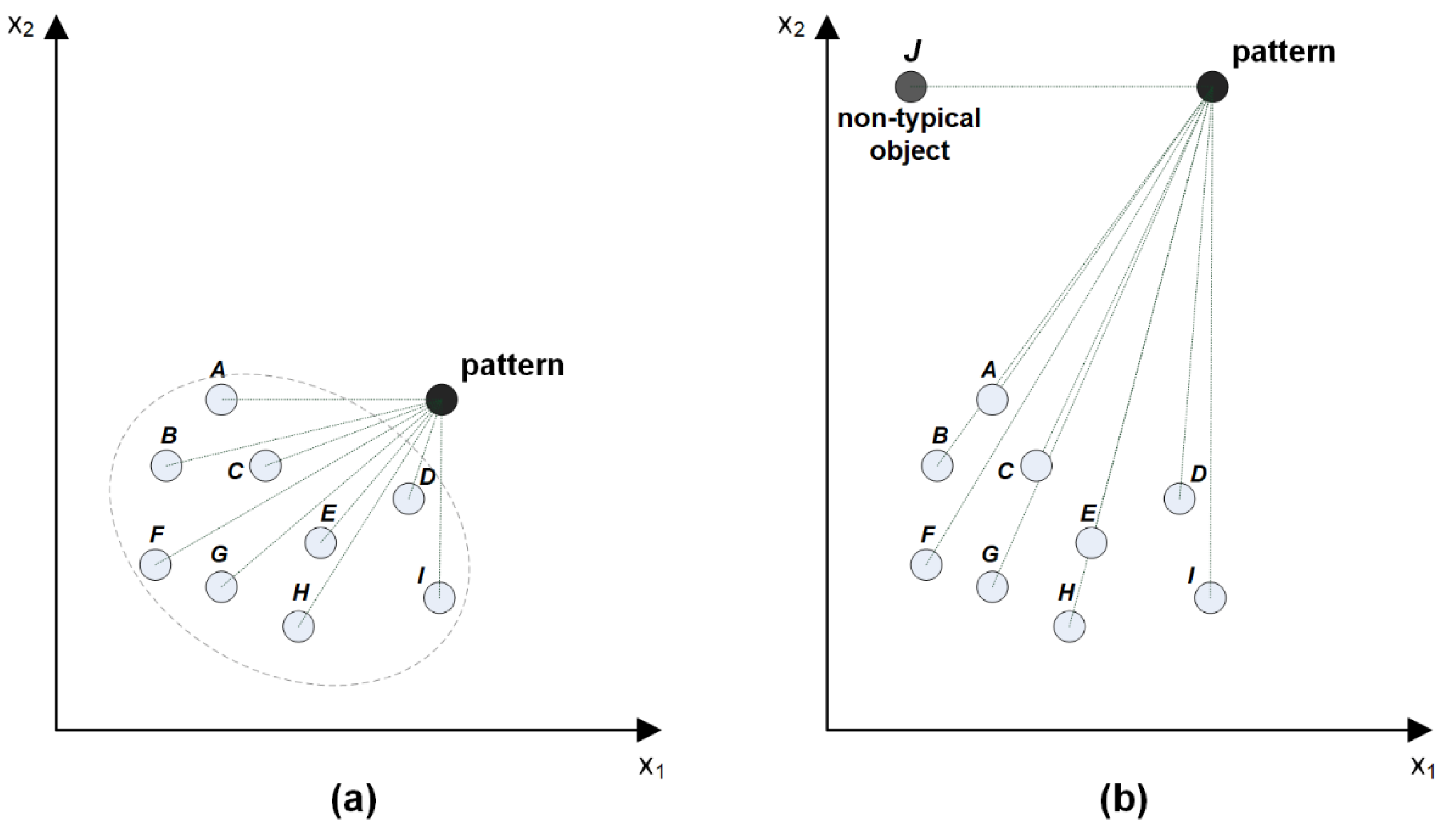
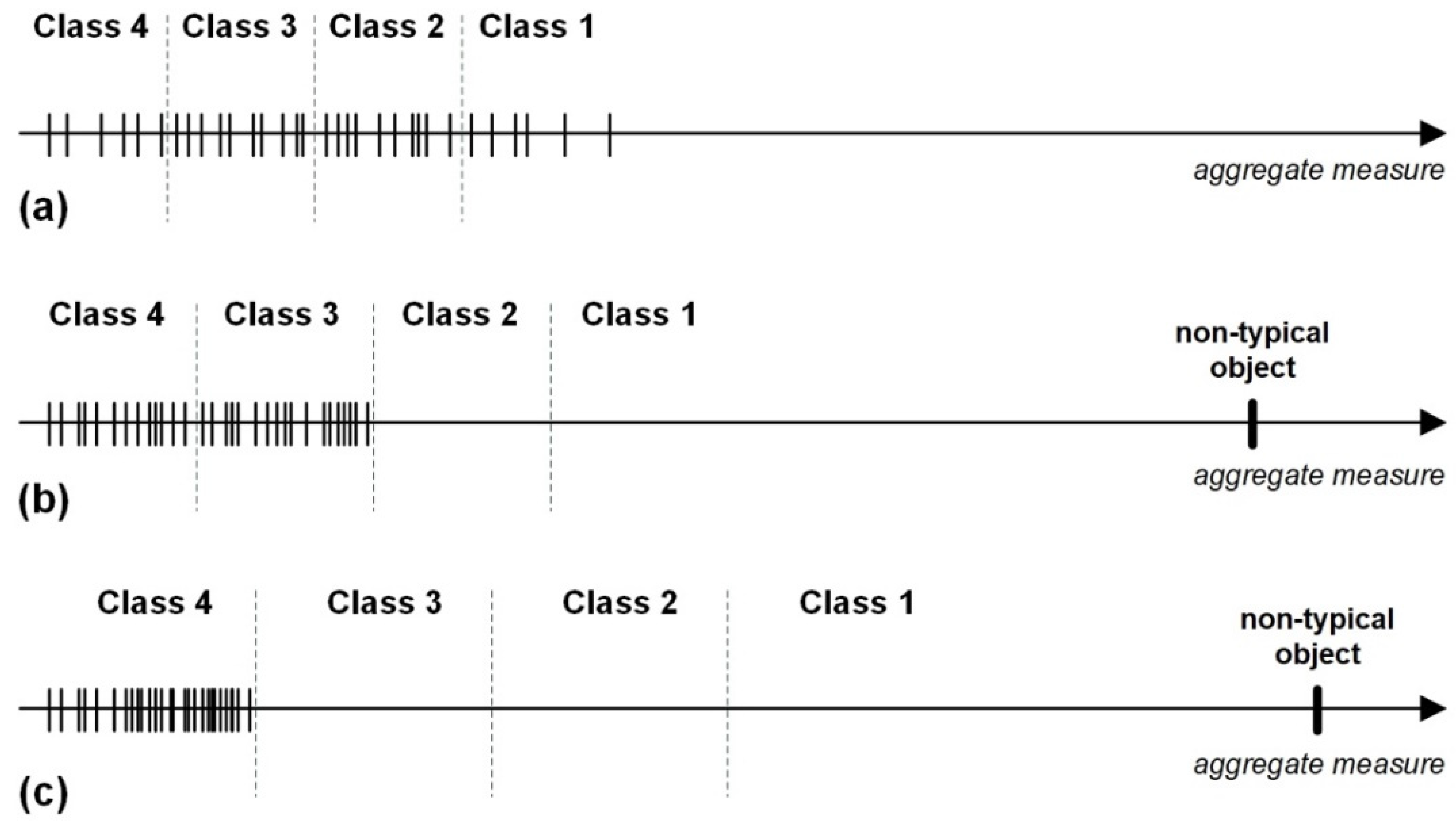
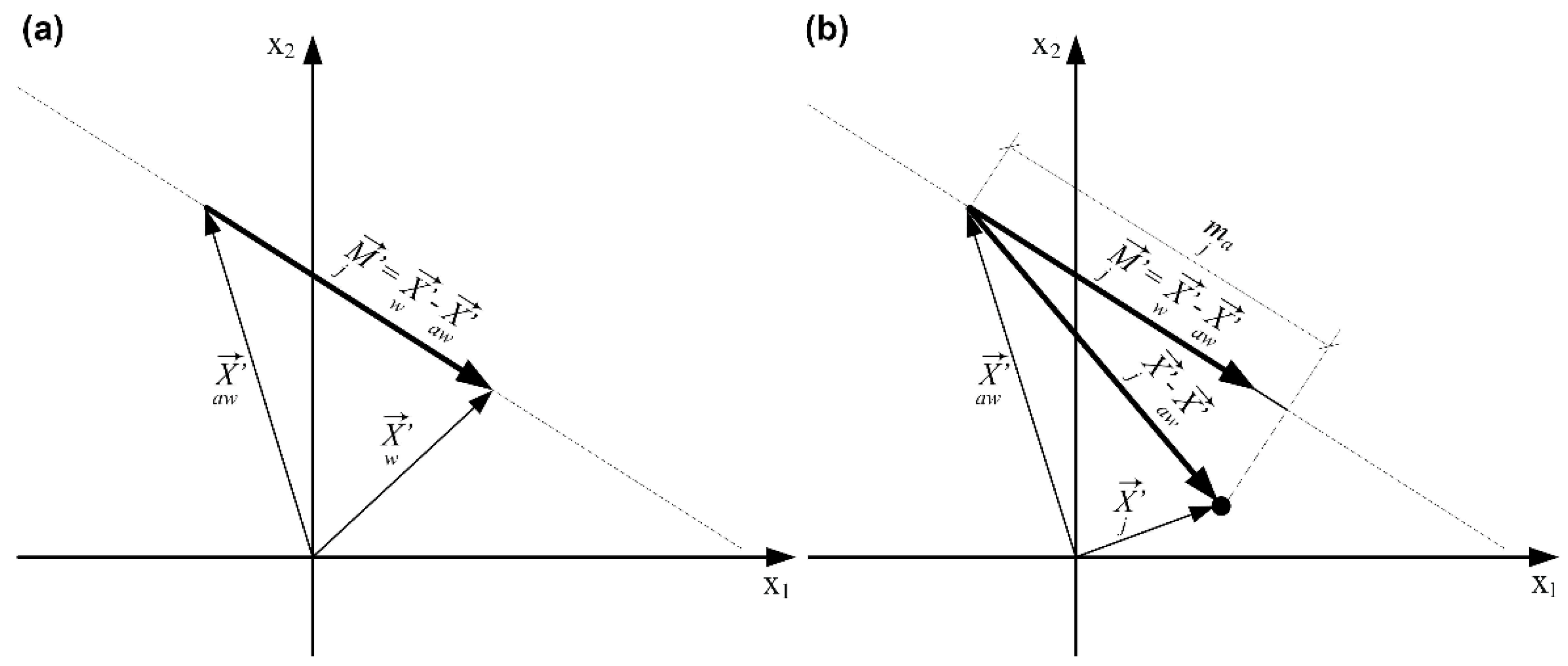
2.1. Theoretical Analysis of the Problem

Sustainable development of energy is one of the most important points of interest in the modern world. It covers many aspects ranging from economic to technological and environmental ones. The complexity of this issue makes this development difficult to assess clearly and objectively [76,77,78,79]. The comparison of the degree of renewable energy development in individual countries requires the construction of appropriate measures to specify its level. To do this, sometimes the existing metrics are used [80], different approaches are combined [81], and different analytic methods are employed, e.g., MCDM/MCDA or MCA. What supports the idea of building new, more customized metrics is the diversity of conditions in which energy development is taking place [82,83]. They are a function of several attributes by which the position of an object relative to other objects can be determined [84,85]. Such metrics are called synthetic measures [86]. They can be represented in a relative or an absolute form [87]. The methods of constructing synthetic measures can be divided into pattern- and anti-pattern-based methods. The concept of the so-called taxonomic measure of development [88,89] is associated with pattern-based methods. It concerns the ordering of the objects under study by their distance from the pattern. This pattern can be an artificially constructed point or a real point. It is usually constructed on the basis of maximum values of variables (stimulants) and minimum (destimulants). The location of the pattern in such a case depends on the location of the extreme elements [89,90,91].
The problem of non-typical objects and their influence on the object classification results are presented in the example of a theoretical analysis. In Figure 1a, an exemplary set of objects (A, B, …, I), which are located near one another (not far apart), is shown. Based on these objects, a pattern was determined. For simplicity, it was assumed that all variables are stimulants, and Euclidean distance was used as a measure of similarity. As it can be seen, the object that is most similar to the pattern (closest) is D, then E, C, I and A. Other objects are slightly further from the pattern, although these disparities are not large. It may also happen that one of the objects is far away from the others. It is known as a non-typical object [86,92]. By adding the non-typical object J to the objects in Figure 1a, we cause the pattern to shift significantly (Figure 1b). This has a considerable effect on ranking the objects according to their similarity to the pattern. In this case, the object most similar to the pattern is J, followed by A, D, C, and B. The presence of non-typical objects can thus significantly affect the ranking of objects in their entire set.
After changing the position of an object with respect to the coordinates, its place in the row may change (to a varying extent). For example, (Figure 2a), when object A moves along the x1 axis, its ranking will not change (A”) or the change will be small (A’). However, when object A is moved along the other axis (x2), the changes in ranking will be significant (Figure 2b). Object A’ has moved away from the pattern by a significant distance and has become ranked the last. Thus, it can be seen that the weights of the variable associated with one axis vary from the weights when the variable is related to the other axis. This is also true for non-typical objects.
The variables involved in creating synthetic measures are often expressed in different measurement units. Thus, they become incomparable. They may also be incomparable due to the different range of values (with the measurement units remaining the same). Then, the procedure of variables normalization is carried out [93,94]. The purpose is to bring the variables to a more or less similar range of values. In the literature, we can find different methods of normalization [94,95,96,97]. These methods are grouped differently [98]. Regardless of the normalization method applied, both the scale of the variables and the position of the objects (value shift) are changed. In general, the aim is to change the scale of variables in such a way that the influence of all the variables on the result of comparison with the pattern is identical.
Similarly, as shown in Figure 1 and Figure 2, the appearance of non-typical objects in the set also affects the normalization result. Normalization methods react differently to non-typical objects. Adding a non-typical value can affect the normalization result in either insignificant or significant way [99]. Some normalization methods reduce values to a preset numerical interval, such as <0–1>, where 0 is the lowest value of the variable and 1 is the highest [80]. The appearance of a value significantly different from the others will increase the weight of this variable. There will also be a further shift of the remaining values. In the case of similarity measures, whose values do not depend on the location of objects in space, this will not have an effect.
Non-typical objects also affect classification. The synthetic measure value of a non-typical object will be significantly different from other objects. On the axis of the synthetic measure value, it will be at a considerable distance from the others. For example, when performing the classification on the basis of standard deviation, we will obtain the extension of the class interval (Class 1, 2, 3, 4) in relation to the absence of a non-typical object (Figure 3).
The classification results in the division into three classes: Class 1 with a non-typical object and Class 3 and Class 4 with objects shifted towards them. In this case, Class 2 is without objects (Figure 3b). As shown in Figure 3c, a situation can occur when there are only two classes: Class 1 with a non-typical object and Class 4 with the remaining objects. In this type of case, more sophisticated classification methods should be used.
The appearance of non-typical objects and their influence on the obtained results (rankings, classifications) is of great practical importance. Although non-typical objects do not appear very often in the analyzed sets, their presence may distort the final results. The world literature describes ways how this issue is addressed [86]. The research conducted by the authors of this paper [99] is one of the examples. In their research, they examined the problem of sustainable development using selected indicators from the defined Sustainable Development Goals (SDGs) [100]. The interpretation of the results obtained in the case of the emerging non-typical objects is very difficult. The weights of the variables depend on the remoteness of the object from other objects. The more the value of a variable describing an object deviates from others, the greater the weight of this variable.

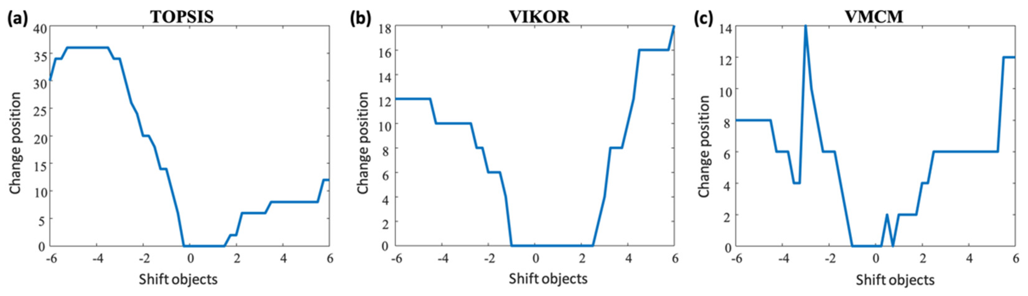
2.2. Practical Verification of the Non-Typical Objects Problem

In order to confirm the problem of non-typical objects in the context of the study on the level of renewable energy generation, experimental research was conducted. The research applied selected real indicators describing the development of renewable energy sources. They were obtained from the IRENA database [101]: X1—Electricity generation (GWh)—Total renewable energy; X2—Electricity generation (GWh)—Hydropower; X3—Electricity generation (GWh)—Renewable hydropower; X4—Electricity generation (GWh)—Wind; X5—Electricity generation (GWh)—Onshore wind energy; X6—Electricity generation (GWh)—Solar; X7—Electricity generation (GWh)—Solar photovoltaic; X8—Electricity generation (GWh)—Bioenergy; X9—Electricity generation (GWh)—Solid biofuels; X10—Electricity generation (GWh)—Other solid biofuels; X11—Electricity generation (GWh)—Biogas. The actual data from the IRENA database on the basis of which the X1–X11 indicators were developed have been shared in the data repository (doi.org/10.6084/m9.figshare.16574855.v1).
Data are for 29 European countries and are from 2018, which to ensure completeness of data for different indicators: Austria (AT), Belgium (BE), Bulgaria (BG), Croatia (HR), Czechia (CZ), Denmark (DK), Estonia (EE), Finland (FI), France (FR), Germany (DE), Greece (EL), Hungary (HU), Ireland (IE), Italy (IT), Latvia (LV), Lithuania (LT), Luxembourg (LU), The Netherlands (NL), Norway (NO), Poland (PL), Portugal (PT), Romania (RO), Slovakia (SK), Slovenia (SI), Spain (ES), Sweden (SE), United Kingdom (UK), Ukraine (UA). The European Union was also added to the pool of objects. A total of 30 objects were obtained.
In this study, the robustness of three MCDM/MCA methods (TOPSIS, VIKOR and VMCM) to the presence of non-typical objects was tested. The TOPSIS and VIKOR are widely used methods (also with regard to RE). The TOPSIS method (Technique for Order Preference by Similarity to Ideal Solution) is dedicated to ordering decision variants, taking into account their similarity to the template (most desirable variant). This is achieved by minimizing the distance from the template (ideal reference solution) and maximizing this distance from the anti-pattern (anti-ideal reference solution). Between each considered variant and the ideal and anti-ideal benchmark distances are determined. They are the determinant of the measure, which takes values from 0 to 1 (0 means the worst object and 1 means the best object). In this way the final order (ranking) is created [102,103]. The VIKOR (serb. VIsekrzterijumska Optimizacija i Kompromisno Resenje) method is used to rank decision-making alternatives and to select a compromise solution when considering conflicting evaluation criteria. For subsequent solutions (variants) the weighted average distance from the best solution is calculated. Next, the maximum weighted distance from this point is determined, and then the comprehensive index is calculated. The obtained values are used to rank the variants (three rankings are created). The variant with the smallest value of the comprehensive index is a proposal for a compromise solution. The compromise solution can also be a set of variants [104,105]. The VMCM (its general assumptions are discussed later in this paper) is an original authors’ method whose applicability has already been proven in many studies [99,106,107,108].
In the first stage of the study, variables were aggregated using three methods: TOPSIS, VIKOR and VMCM. The ranking position of each object was determined. In the second stage, in order to simulate the appearance of a non-typical object in the sample, the values of the variables for subsequent objects were changed (from −6σ to + 6σ—of standard deviations of the original value). The standard deviations were counted for all values of variables for all objects. As a result of the simulation, one object (Finland) and one variable (X6, Electricity generation (GWh), Solar photovoltaic) were selected. The values of standard deviation were changed with a step of 0.25. For each case, the variable was aggregated for the selected methods. The rankings were made on the basis of the value of the aggregate measure developed, as a result of aggregating indicators X1–X11. The higher the values of the measure for a given country, the higher this country is in the ranking created. This means that a given country is closer to the adopted benchmark object and further from the anti-benchmark. The stability of classification was examined by checking how many objects changed their position in the ranking and by how much they changed in comparison to the result obtained in the first stage.
The results for the TOPSIS, VIKOR and VMCM are illustrated in Figure 4. The ordinate shows by how far all the objects were shifted from their ranking position. This was calculated by summing the differences in positions of all the objects from their original ranking. For example, in Figure 4a, in the case of the TOPSIS method, the change in one coordinate (X6, Electricity generation (GWh), Solar photovoltaic) of the object Finland by −2σ results in shifting of all the objects (described in Table 1) by 20 positions. In contrast, in the case of the VIKOR method all the objects are shifted by six positions, similarly to the VMCM.
With regard to the TOSPSIS method (Table 1), after the change of values by −6 of standard deviations, Bulgaria went up by five positions (from 19 to 14) while Greece went up by four positions (from 12 to 8). Six other objects were shifted by two positions: Sweden (from 7 to 9), Italy (from 9 to 11), Croatia (from 13 to 15), Ireland (from 14 to 16), Spain (from 15 to 13) and Czechia (from 17 to 19). The other nine objects moved up by one position: Norway (from 3 to 4), Germany (from 4 to 3), Estonia (from 8 to 7), Europe (from 11 to 12), Romania (from 16 to 17), Lithuania (from 23 to 24), France (from 24 to 23), Hungary (from 25 to 26) and Luxembourg (from 26 to 25).
As far as the VIKOR method is concerned (Table 2), after the change in values by −6 standard deviations, Romania was shifted upwards by three positions (from 20 to 17). None other objects moved by one position: Germany (from 4 to 5), Denmark (from 5 to 4), Czechia (from 14 to 15), Estonia (from 15 to 14), Greece (from 17 to 18), Lithuania (from 18 to 19), Ireland (from 19 to 20), The Netherlands (from 24 to 25) and Slovenia (from 25 to 24). The remaining objects remained at their previous positions.
As regards the VMCM (Table 3), after the change of values by −6 standard deviations, two objects went up by two positions: Spain (from 13 to 11) and Romania (from 12 to 14). The other four objects moved by one position: Sweden (from 8 to 7), Italy (from 7 to 8), Croatia (from 11 to 12), and Greece (from 14 to 13). The remaining sites did not change their position.
The above research results demonstrate that the appearance of a non-typical object in the research sample can significantly affect the final results. As a consequence, the picture of reality may be distorted and wrong conclusions may be drawn, thus leading to incorrect interpretation. Referring to the scope of the analysis based on selected indicators, it may turn out that the obtained ranking does not represent the actual level of development of renewable energy sources in particular countries. Therefore, it should be kept in mind that the choice of a proper research method (even from the popular ones) is very important. The research shows that the proposed VMCM copes with non-typical objects much better than the two other methods under scrutiny.
Therefore, the authors suggest the use of the VMCM in studies on the level of development (generation) of renewable energy in individual countries (these can also be regions or other areas resulting from administrative divisions). With such complex multivariate analyses (many objects and variables), outliers are bound to appear in the source data. In addition to the robustness of the VMCM to non-typical objects, it permits examination of the dynamics of change as well as comparison of results from year to year. It also offers the possibility to relate changes of objects to real objects that are reference points. Details of the study on the development dynamics and a detailed mathematical description of the VMCM, including the comparability of rankings across years, were presented by the authors in their previous works [99,106,107].

3. Materials and Methods

The authors applied the VMCM to study the level of energy production from renewable sources in selected European countries. This method meets the requirements that have been set out in the section concerning the purpose of the paper. What is more, it offers the opportunity to study changes from a dynamic perspective.
The study used the same indicators as in the (previous) study on the robustness of the methods to non-typical objects, namely X1—Electricity generation (GWh)—Total renewable energy; X2—Electricity generation (GWh)—Hydropower; X3—Electricity generation (GWh)—Renewable hydropower; X4—Electricity generation (GWh)—Wind; X5—Electricity generation (GWh)—Onshore wind energy; X6—Electricity generation (GWh)—Solar; X7—Electricity generation (GWh)—Solar photovoltaic; X8—Electricity generation (GWh)—Bioenergy; X9—Electricity generation (GWh)—Solid biofuels; X10—Electricity generation (GWh)—Other solid biofuels; X11—Electricity generation (GWh)—Biogas. These indicators were selected with the use of the expert method. The data were obtained from the IRENA database [101] and they the period 2001–2018 (due to the completeness of data concerning the selected indicators). The data referred to renewable energy generation in 29 European countries: Austria (AT), Belgium (BE), Bulgaria (BG), Croatia (HR), Czechia (CZ), Denmark (DK), Estonia (EE), Finland (FI), France (FR), Germany (DE), Greece (EL), Hungary (HU), Ireland (IE), Italy (IT), Latvia (LV), Lithuania (LT), Luxembourg (LU), The Netherlands (NL), Norway (NO), Poland (PL), Portugal (PT), Romania (RO), Slovakia (SK), Slovenia (SI), Spain (ES), Sweden (SE), United Kingdom (UK) and Ukraine (UA).
In the study, the Vector Measure Construction Method (VMCM) was employed. The effectiveness of this method with regard to non-typical objects has been confirmed by previous studies. The VMCM uses the properties of vector calculus to construct a synthetic measure in dynamic terms. Moreover, it allows ranking with respect to artificial or real reference points. A detailed description of the method can be found, e.g., in the work [106], while the main stages of the procedure are discussed below. The computational procedure of the VMCM is as follows:
  • Stage 1. Selection of diagnostic variables.
  • Stage 2. Elimination of indicators.
  • Stage 3. Identification of the nature of diagnostic variables.
  • Stage 4. Assigning weights to the diagnostic variables.
  • Stage 5. Normalization of variables.
  • Stage 6. Determination of pattern and anti-pattern.
  • Stage 7. Building a synthetic measure.
  • Stage 8. Classification of objects.
In the first stage, 11 indicators describing types of renewable energy generation sources in 29 selected European countries were selected. In the second stage, indicators characterized by a sufficiently high coefficient of variation were chosen. Variables with too low a coefficient of variation were eliminated. In the next step, the character of variables was determined, which concerns assigning diagnostic variables to one of three groups, namely stimulants, destimulants and nominants. The stimulants were such variables whose higher values indicated a higher level of development of the analyzed phenomenon (renewable energy). The destimulants were variables whose lower values indicated a higher level of development, for example, due to the type of energy source. The nominants were variables whose desired values were within a certain numerical range. In the analyzed example, high values of the considered indicators positively affected the level of development of alternative energy sources. Therefore, all indicators were stimulants. All variables were assigned equal weights. Standardization was used as a method of normalization. At the same time, the mean value and standard deviation were counted for indicators from all considered years. In order to reduce the number of non-typical objects affecting the ranking results, the pattern was calculated on the basis of quartiles. Such a pattern is less sensitive to non-typical objects and thus more representative of objects with typical indicator values. The pattern has coordinate values that are the first quartile for indicators that are destimulants and the third quartile for indicators that are stimulants. The coordinate values of the anti-pattern were counted based on the first quartile for indicators having the nature of stimulants and the third quartile for indicators having the nature of destimulants. The most important step of the VMCM method is the construction of a synthetic measure to assess the level of renewable energy generation. The VMCM synthetic measure is characterized by transparency and simplicity of interpretation when comparing the pattern and anti-pattern to all the objects in the research sample. This is due to the use of vector calculus properties. The measure is expressed as a component of a vector representing the object along a differential vector M j , which is the difference between the vector-pattern and X w vector-anti-pattern ( X a w  Figure 5a). The vector M j determines a one-dimensional coordinate system with origin in the point determined by the end of the vector X a w . The synthetic measure is m a j the value of the projection of the vector X j X a w onto the vector M j (Figure 5b). It allows us to tell how much longer (better) or shorter (worse) the vector representing the object is than the differential vector.
Due to using the properties of vector calculus, the VMCM offers more possibilities than distance measures. Distance measures are more difficult to interpret, and objects cannot be better than a pattern. The last stage of the VMCM method is the division of objects into classes with similar measure values. This makes the results more clear to read and facilitates graphical presentation. A good solution for spatial object ranking is a map-like solution that is easier to present. Objects are visualized using colors that reflect the classes. The division of objects into classes can be made on the basis of, for instance, the mean value and standard deviation of the m ¯ m a 0 synthetic measure σ m a 0 . Four classes are then formed and specific objects are assigned [109]:
{ 1   for   m a j m ¯ m a 0 + σ m a 0 ;   )   ,   2   for   m a j m ¯ m a 0 ; m ¯ m a 0 +   σ m a 0 )   , 3   for   m a j m ¯ m a 0 σ m a 0 ;   m ¯ m a 0 )   ,   4   for   m a j ( ; m ¯ m a 0 σ m a 0 )   .  
Using quantiles, objects can be divided into any number of classes.

4. Results and Discussion

Firstly, the level of renewable energy generation by European countries from 2001 to 2018 was investigated in dynamic terms. The base year was chosen to be 2009, because in 2001–2007, the values of two diagnostic variables (X6—Electricity generation (GWh)—Solar; X7—Electricity generation (GWh)—Solar photovoltaic) were very low compared to 2014–2018. Large differences in the values of these variables could blur the picture of reality for the obtained ranking. At the stage of the diagnostic variables normalization, their values would have been artificially increased. This would have resulted in their impact on the measure being greater than desired. Therefore, due to their small values, they should be eliminated at the second stage of the research procedure performed with the VMCM (variable elimination). Nevertheless, year by year, solar technology is becoming more and more important among renewable energy sources. It is difficult to compare its share in 2001 and, for example, several years later. In order to be able to investigate in the research the whole period of 2001–2018, the base year was changed from 2001 to 2009. In that year, the values of the above-mentioned variables (X6, X7) reached much higher values. Since 2009, an increase in solar energy generation could be seen very clearly in the majority of the European countries. Next, the mean values and standard deviations were calculated from the 2009 data and used to normalize the indicator values for the following years. An artificial pattern and anti-pattern were constructed according to stage six of the VMCM. The pattern and anti-pattern were established on the basis of quartiles calculated for the base year 2009. All objects in subsequent years were ranked in relation to that pattern and anti-pattern. In the next stage, objects were divided into classes. The division into four classes (very good, good, medium, poor) was introduced in order to present the level of development of individual countries more clearly. It is easier to compare the positions of countries with a similar level of renewable energy development. The creation of four classes was also dictated by the fact that, in this type of research (MCA methods), it is often this number that is distinguished. Class ranges were determined according to formula (1), with the mean and standard deviation calculated for the base year. Based on these, the class ranges adopted for the classification for all subsequent years were determined. Table 4 shows the results of the rankings of the European countries of 2001, 2009 and 2018 made with the use of the VMCM with respect to the artificial pattern constructed on the basis of the values of the 2009 indicators.
In 2001, Finland (FI) was assigned to Class 1. Class 2 contained Austria (AT), Norway (NO), Sweden (SE) and Denmark (DK), while Class 3 included Latvia (LV), Croatia (HR), Portugal (PT), the UK (UK), Slovenia (SI), Spain (ES), Romania (RO), Slovakia (SK), The Netherlands (NL), Italy (IT) and France (FR). Class 4 consisted of Germany (DE), Czechia (CZ), Poland (PL), Ireland (IE), Greece (EL), Luxembourg (LU), Belgium (BE), Bulgaria (BG), Lithuania (LT), Ukraine (UA), Estonia (EE) and Hungary (HU). In 2009, Class 1 contained Austria (AT), Spain (SE), Denmark (DK), Finland (FI), and Norway (NO). In Class 2, there were the UK (UK), Germany (DE), Spain (ES), Hungary (HU), Portugal (PT) and The Netherlands (NL), while Class 3 included Latvia (LV), Estonia (EE), Slovenia (SI), Belgium (BE), Italy (IT), Croatia (HR), Czechia (CZ), Ireland (IE), Slovakia (SK), Poland (PL), Romania (RO), France (FR), Greece (EL), Lithuania (LT) and Luxembourg (LU). In Class 4, there were Bulgaria (BG) and Ukraine (UA). In 2018, the UK (UK), Denmark (DK), Germany (DE), Estonia (EE), Finland (FI), Latvia (LV), Austria (AT), Sweden (SE), Italy (IT), Norway (NO), Portugal (PT), Czechia (CZ), Spain (ES), Belgium (BE) and Bulgaria (BG) entered Class 1, while Class 2 consisted of Croatia (HR), Greece (EL), Ireland (IE), Slovakia (SK), Romania (RO), Lithuania (LT), The Netherlands (NL), Hungary (HU), Slovenia (SI) and France (FR), Class 3 consisted of of Luxembourg (LU) and Poland (PL), and Class 4 consisted of Ukraine (UA).
In the UK, since 2001 there was a 1376% increase in the capacity for renewable-energy-generating facilities, which shifted the country from ninth place in the ranking to first place in 2018. In 2001, hydroelectricity provided most of the green energy in the UK and other countries. Investments in other renewable energy sources led to a situation where the proportion of the British hydroelectric capacity to the capacity of all the power-generating facilities in the country dropped to just 10%. The most striking increase in the UK was seen in the number of solar power facilities. Between 2001 and 2018, the increase in their capacity amounted to 437,278%, and its share in the total power generated by renewables rose from 0.09% to about 30%. The capacity share of wind power facilities increased from 15% to about 50% (4416% increase in their capacity). The smallest rise in capacity was seen in biofuels and biogas, where, despite significant increases in the facility capacity, their share remained marginal.
Finland, after being a ranking leader in 2001, fell to the 5th position in 2018. This was mainly due to poor conditions for solar energy production. The capacity for renewable-energy-generation facilities rose only by 166%. Energy from hydroelectric power still played a dominant role there, even though its share in the total power generated by renewable sources fell from 63% to 42%. The share of solar energy was still small as it rose from 0.06% to 1.85%. The most noticeable increase took place in the capacity of wind-energy-generating facilities, rising from 0.84% to 26%.
Germany was ranked 17th in 2001 and jumped to the 3rd position in 2018. The capacity of renewable energy production facilities soared to 805%. In 2001, wind and hydroelectric-generating facilities were dominant. In 2018, the share of hydroelectric capacity in all renewables fell below 10%, while wind (50% share) and solar (38% share) power-generating facilities play a dominant role, with their 50% and 38% shares, respectively.
Estonia moved upwards from penultimate place in 2001 to fourth in 2018. Over that period, the country saw an 8693% increase in the capacity of renewable energy generation facilities. Bioenergy was dominant in 2001 (capacity share at 71%). The second most popular power facilities were hydroelectric power plants (with capacity share at 29%). Other energy sources were not exploited. By 2018, the largest investments were made in wind energy facilities. As a result, in 2018, these wind farms prevailed with their capacity share at 51%. The proportion of bioenergy capacity fell to 43%, while hydroelectricity dropped to 1.2%. Some investment was made in solar power generation, but its capacity was still relatively small (5.2%).
The Netherlands dropped in the ranking from 14th position in 2001 to 22nd position in 2018. The increase in the facilities’ capacity was 1244%. The low ranking was due to the low ratio of renewable energy facility capacity to the energy consumed. The ratio in 2018 was only 18% for the top ranking country, i.e., the UK. Due to the lack of suitable conditions, the share of the capacity of hydroelectric facilities was only 4.7% in 2001, and in 2018 it dropped even further to 0.38% (in renewable energy sources). In 2001, wind and bioenergy-generating facilities were dominant, while in 2018 the leading sectors were wind (45%) and solar (46%) generating facilities.
In France, the increase in power capacity was relatively small (210%), which resulted in a drop from 16th (2001) to 25th place (2018). Hydroelectric plants were dominant in 2001 with a capacity share close to 100%. The share of wind and solar power capacity was 0.16% and 0.03%, respectively. The proportion of bioenergy did not exceed 2%. In 2018, investment in wind and solar power generation facilities brought their capacity share to 30% and 19%, respectively, in 2018. Hydroelectric plants retained their dominant position (48%).
Poland fell from its 19th position (2001) in the ranking to the penultimate position in 2018. This was due to a very low ratio of the capacity of renewable energy generation facilities to the energy consumed. That ratio was 16.19% in relation to the best ranked UK. In 2001, hydroelectric plants played a dominant role. Their capacity accounted for 95% of the capacity of all the renewable energy generating facilities in the country. The share of wind and bioenergy capacity was marginal (2% and 3%, respectively). There were no solar-power-generation facilities. In the following years, significant investments were made in wind power generation, making it a dominant source of renewable energy with a capacity share at 69% in 2018. Investments in solar power generation facilities were insignificant compared to other countries (capacity share in 2018 was at 6.7%).
Figure 6a shows that in 2001 there was a clear division into the northern, western and eastern European countries. In 2001, the northern European countries generated energy from renewable sources at high and medium levels. In the western European countries, that level was low and very low (with the exception of Austria) while in the eastern European countries the renewable energy generation level was very low. This indicates that environmental awareness was higher in northern and western European countries than in the east of Europe. The investments made between 2001 and 2018 changed that situation (Figure 6a and Figure 7a,b). The western European countries gradually caught up with the northern European countries to outpace them later. This was partly due to the unfavorable conditions regarding solar energy generation in the north of Europe.
The difference between the pattern and the anti-pattern determines the ranking order of the objects. The greater the difference is for a given variable, the more this variable affects the ranking result. Table 5 shows the values of variables after normalization for the pattern (UK) and the anti-pattern (Ukraine). The values of the variables for Ukraine are very small, close to zero, so they do not have much influence on the ranking result. The main influence comes from the values of the UK variables.
The difference between the values of the pattern and the anti-pattern shows that the variable X1—Electricity generation (GWh)—Total renewable energy had the greatest impact on the ranking and was the determining factor for the ranking position. The second most important factor was the amount of wind energy produced, represented by the variable X4—Electricity generation (GWh)—Wind. This is due to the specific geographical location of the UK on the island, so that the country has very good access to sites favorable for wind energy production. A little less important, but still quite significant, was the production of bioenergy, whereas the production of hydroelectric power could be considered of marginal importance. Its share in the mix was gradually decreasing, which was due to the low availability of places where such energy could be generated as well as to the negative environmental impact of large investments of this kind. The unquestionable advantage of hydroelectric power plants is the constant and uninterrupted access to energy independent of environmental factors. The low values for the variables related to solar energy were due to a rather uniform situation when regarding solar energy installations. Technological breakthroughs, easy installation and the possibility of mounting small systems for individual households mean that there is a boom in the market for solar installations almost all over Europe. This results in a fairly similar situation across Europe with some exceptions. This again made the variables related to solar energy production poorly differentiated between countries, which translated into an automatic decrease in its importance.
Table 6 shows the ranking made with the use of the real pattern (UK) and anti-pattern (AU) from 2018. The top-ranking countries did not change their positions. This was because the pattern of investment in renewable energy generation facilities in the UK was in line with the overall European trend. All countries in the top tier that can be considered leaders are making investments in a similar way. Due to huge changes in renewable energy generation and investments, resulting in capacity being boosted by hundreds of percent, older installations constructed in line with the approach to renewables prevalent in the late 20th century have a small share of the total energy mix.
An example of a country that changed its position in the new ranking is Italy. In 2018, it moved from position 9 to position 7. This was due to the very high rate of capacity of renewable energy production facilities to energy consumed. As regards Italy, this variable had the highest value, and at the same time, in the new ranking, this variable gained the highest importance. In the previous ranking, it was a variable equivalent to the variable representing wind energy production, and it was less significant than bioenergy production.
Norway is one of the countries whose position in the ranking dropped. It fell from 10th to 18th place. In Norway, hydroelectric power plants are the dominant source of renewable energy. In 2018, their capacity share was 96% of total renewables. This was due to the country’s specific geographical conditions, but it did not fit into the pan-European trend. Investment in other renewables was very low compared to other countries, but thanks to hydroelectricity, Norway enjoyed the highest ratio of power generating facilities capacity to energy consumption.
Figure 8 and Figure 9 show the result of the classification with the use of the real pattern and the anti-pattern. It can be seen that in 2018, a group of countries from southeastern Europe emerged, where investments in renewable energy were lower than in other European countries. The worst situation was seen in Ukraine, Poland and Slovenia. In Western European countries, however, the clear outlier is France.
Figure 10 shows the spread of measure values between 2001 and 2018. The large increase in the value of resources was due to a large increase in the number of renewable energy sources. This resulted in a very significant increase in the share of renewable energy in energy consumption. This increase was mainly in wind, solar and to a slightly lesser extent bioenergy. The increase in the number of hydropower plants was small compared to other facilities.
The largest increase in renewables was in Germany and the smallest in Ukraine. The effect of the growth in Germany can be seen in the graph showing the situation in 2013, but growth also occurred in earlier years. There are only two countries above the mean curve in the graph, namely Germany and the UK. These are the countries that were assigned to Class 1 in 2018. Several Class 2 countries were also above average, but not shown in the graph.

5. Conclusions

The MCDM/MCDA multicriteria analysis and MCA multivariate comparative analysis methods are excellent tools for decision support in the context of evaluating and studying the sustainability of renewable energy. The MCA methods take into account the complexity, multidimensionality and long-term nature of renewable energy development and support decision-making processes. They are based on a variety of measures (existing and newly developed), which, when appropriately selected, helps to include in considerations the whole range of conditions for the development of renewable energy sources. However, the data included in the analyses can be characterized by diversity, i.e., the same variables can adopt small and large values. The so-called non-typical objects appearing in this way may affect the correctness of the results obtained with the use of the methods of multivariate analysis.
The methodological solution proposed by the authors should be considered as innovative. The author’s VMCM method effectively solves the problem of atypical objects (it performs much better than the analyzed TOPSIS and VIKOR methods). Moreover, thanks to the unique approach to pattern construction, it allows one to study the dynamics of changes over time. The used aggregate measure is not limited in the multidimensional space (from below and above), so there is a possibility to take into account objects better than the adopted pattern. It also allows the construction of aggregate measures using arbitrary indicator configurations.
The research presented here on the level of development of renewable energy sources in European countries has shown the effectiveness of the proposed method in this regard. When assuming different patterns and anti-patterns (artificial and real) and different base (reference) years, interesting results were obtained for the countries (objects) under consideration. They allow for detailed analyses of development trends over a number of years. This gives a fairly complete picture of the phenomenon of renewable energy development in the adopted scope. The measures included in the study can be freely modified (extended or narrowed) by changing the sets of diagnostic variables, e.g., the ones describing the levels of renewable energy consumption in relation to the level of its generation. This, in turn, will make it possible to look at this phenomenon from yet another angle. The VMCM has also proven to be sensitive to changes in data values and more effective in different situations when, for example, the analysis needs to be completed with new variables or new sources of energy need to be considered, as well as when changes are necessary due to new legislation.
The proposed solution can be used to support decision-making at different levels, e.g., regional, national or European (as presented in the paper). The results can be used by decision makers (e.g., at the European level) when planning subsidies for the sustainable development of renewable energies. The resulting rankings (based on a developed aggregate measure for selected indicators) make it possible to determine the level of renewable energy development in individual countries (in different time periods). The division of countries into classes allows the grouping of countries with a similar level of development, comparing possibilities in relation to, for example, the most developed ones and making decisions about possible support for specific forms of renewable energy development.
MCA methods (TOPSIS, VMCM) are dedicated to the analysis of large numbers of data, covering a large number of objects and evaluation criteria. They do not require the active participation of the decision maker in the calculation procedure. The main limitation of this type of research may be the partial lack of data. Available databases, such as IRENA, EUROSTAT, etc. sometimes contain data gaps. Some data for some indicators or particular years are missing. Another limitation may be the low variability of values of criteria, taken into account while constructing the aggregate measure.

Author Contributions

Conceptualization, M.P., M.B. and K.N.; methodology, M.P., M.B. and K.N.; software, M.B.; validation, K.N.; formal analysis, M.P., M.B. and K.N.; investigation, M.P., M.B. and K.N.; resources, M.P. and K.N.; data curation, M.P., M.B. and K.N.; writing—original draft preparation, M.P., M.B. and K.N.; writing—review and editing, M.P., M.B. and K.N.; visualization, M.B. and K.N.; supervision, M.P., M.B. and K.N.; project administration, M.P., M.B. and K.N. All authors have read and agreed to the published version of the manuscript.

Funding

This research was funded by Institute of Management, University of Szczecin.

Institutional Review Board Statement

Not applicable.

Informed Consent Statement

Not applicable.

Data Availability Statement

The source data relative to the study could be obtained at: doi.org/10.6084/m9.figshare.16574855.v1.

Conflicts of Interest

The authors declare no conflict of interest. The funders had no role in the design of the study; in the collection, analyses, or interpretation of data; in the writing of the manuscript; or in the decision to publish the results.

References

  1. Munasinghe, M. Sustainable Development: Basic Concepts and Application to Energy. In Encyclopedia of Energy; Cleveland, C.J., Ed.; Elsevier: New York, NY, USA, 2004; pp. 789–808. ISBN 978-0-12-176480-7. [Google Scholar]
  2. UN General Assembly. Transforming Our World: The 2030 Agenda for Sustainable Development. Available online: https://www.refworld.org/docid/57b6e3e44.html (accessed on 28 June 2021).
  3. McCollum, D.; Gomez Echeverri, L.; Riahi, K.; Parkinson, S. Sdg7: Ensure access to affordable, reliable, sustainable and modern energy for all. In A Guide to SDG Interactions: From Science to Implementation; Griggs, D.J., Nilsson, M., Stevance, A., McCollum, D., Eds.; International Council for Science: Paris, France, 2017; pp. 127–173. [Google Scholar]
  4. Statista. Leading Countries in Installed Renewable Energy Capacity Worldwide in 2020. Available online: https://www.statista.com/statistics/267233/renewable-energy-capacity-worldwide-by-country (accessed on 20 July 2021).
  5. Li, L.; Lin, J.; Wu, N.; Xie, S.; Meng, C.; Zheng, Y.; Wang, X.; Zhao, Y. Review and Outlook on the International Renewable Energy Development. Energy Built Environ. 2020. [Google Scholar] [CrossRef]
  6. European Commission. EU ETS Handbook. Available online: https://ec.europa.eu/clima/sites/default/files/docs/ets_handbook_en.pdf (accessed on 16 July 2021).
  7. European Commission. Directive (EU) 2018/2001 of the European Parliament and of the Council of 11 December 2018 on the Promotion of the Use of Energy from Renewable Sources (Recast) (Text with EEA Relevance). Available online: https://eur-lex.europa.eu/eli/dir/2018/2001/2018-12-21 (accessed on 16 July 2021).
  8. European Commission. Directive (EU) 2018/2002 of the European Parliament and of the Council of 11 December 2018 Amending Directive 2012/27/EU on Energy Efficiency (Text with EEA Relevance). Available online: https://eur-lex.europa.eu/eli/dir/2018/2002/oj (accessed on 16 July 2021).
  9. European Commission. Directive (EU) 2019/944 of the European Parliament and of the Council of 5 June 2019 on Common Rules for the Internal Market for Electricity and Amending Directive 2012/27/EU (PE/10/2019/REV/1). Available online: https://eur-lex.europa.eu/eli/dir/2019/944/oj (accessed on 16 July 2021).
  10. European Commission. Communication from the Commission to the European Parliament, the European Council, the Council, the European Economic and Social Committee and the Committee of the Regions. The European Green Deal. Available online: https://eur-lex.europa.eu/legal-content/EN/TXT/?qid=1576150542719&uri=COM%3A2019%3A640%3AFIN (accessed on 16 July 2021).
  11. Komarnicka, A.; Murawska, A. Comparison of Consumption and Renewable Sources of Energy in European Union Countries—Sectoral Indicators, Economic Conditions and Environmental Impacts. Energies 2021, 14, 3714. [Google Scholar] [CrossRef]
  12. Štreimikienė, D. Externalities of Power Generation in Visegrad Countries and Their Integration through Support of Renewables. Econ. Sociol. 2021, 14, 89–102. [Google Scholar] [CrossRef]
  13. European Commission. Commission Delegated Regulation (EU) 2021/340. Available online: https://eur-lex.europa.eu/eli/reg_del/2021/340/oj (accessed on 29 August 2021).
  14. International Renewable Energy Agency; European Commission. Global Energy Transformation: A Roadmap to 2050; International Renewable Energy Agency (IRENA): Masdar City/Abu Dhabi, United Arab Emirates, 2019; ISBN 978-92-9260-121-8. [Google Scholar]
  15. Santos, A.Q.O.; da Silva, A.R.; Ledesma, J.J.G.; de Almeida, A.B.; Cavallari, M.R.; Junior, O.H.A. Electricity Market in Brazil: A Critical Review on the Ongoing Reform. Energies 2021, 14, 2873. [Google Scholar] [CrossRef]
  16. das Minas, B.M.; Energia; da Infra-Estrutura, B.M.; de Energia, B.S. Balanço Energético Nacional. Ministério das Minas e Energia. 2003. Available online: http://www.agg.ufba.br/ben2003/BEN2003_port.pdf (accessed on 13 September 2021).
  17. Empresa de Pesquisa Energética (EPE). Plano Nacional de Energia 2030. Available online: http://antigo.mme.gov.br/documents/36208/468569/Plano+Nacional+de+Energia+2030+%28PDF%29.pdf/b22cf6a2-8d5f-5c5b-dd3a-414381890002 (accessed on 16 July 2021).
  18. Guo, X.; Guo, X. China’s Photovoltaic Power Development under Policy Incentives: A System Dynamics Analysis. Energy 2015, 93, 589–598. [Google Scholar] [CrossRef]
  19. Ministry of Foreign Affairs, PRC. Statement by Xi Jinping President of the People’s Republic of China at the General Debate of the 75th Session of the United Nations General Assembly. Available online: https://www.fmprc.gov.cn/mfa_eng/zxxx_662805/t1817098.shtml (accessed on 20 July 2021).
  20. US Energy Information Administration. Monthly Energy Review. Available online: https://www.eia.gov/totalenergy/data/monthly (accessed on 19 July 2021).
  21. US Energy Information Administration. Annual Energy Outlook 2021. Available online: https://www.eia.gov/outlooks/aeo/pdf/AEO_Narrative_2021.pdf (accessed on 21 July 2021).
  22. Vo, D.H. Sustainable Agriculture & Energy in the U.S.: A Link between Ethanol Production and the Acreage for Corn. Econ. Sociol. 2020, 13, 259–268. [Google Scholar] [CrossRef]
  23. Menyah, K.; Wolde-Rufael, Y. CO2 Emissions, Nuclear Energy, Renewable Energy and Economic Growth in the US. Energy Policy 2010, 38, 2911–2915. [Google Scholar] [CrossRef]
  24. Ellabban, O.; Abu-Rub, H.; Blaabjerg, F. Renewable Energy Resources: Current Status, Future Prospects and Their Enabling Technology. Renew. Sustain. Energy Rev. 2014, 39, 748–764. [Google Scholar] [CrossRef]
  25. Kaygusuz, K. Wind Power for a Clean and Sustainable Energy Future. Energy Sources Part B Econ. Plan. Policy 2009, 4, 122–133. [Google Scholar] [CrossRef]
  26. Adekoya, O.B.; Olabode, J.K.; Rafi, S.K. Renewable Energy Consumption, Carbon Emissions and Human Development: Empirical Comparison of the Trajectories of World Regions. Renew. Energy 2021, 179, 1836–1848. [Google Scholar] [CrossRef]
  27. Solangi, Y.A.; Longsheng, C.; Shah, S.A.A. Assessing and Overcoming the Renewable Energy Barriers for Sustainable Development in Pakistan: An Integrated AHP and Fuzzy TOPSIS Approach. Renew. Energy 2021, 173, 209–222. [Google Scholar] [CrossRef]
  28. Richards, G.; Noble, B.; Belcher, K. Barriers to Renewable Energy Development: A Case Study of Large-Scale Wind Energy in Saskatchewan, Canada. Energy Policy 2012, 42, 691–698. [Google Scholar] [CrossRef]
  29. Adhikari, S.; Mithulananthan, N.; Dutta, A.; Mathias, A.J. Potential of Sustainable Energy Technologies under CDM in Thailand: Opportunities and Barriers. Renew. Energy 2008, 33, 2122–2133. [Google Scholar] [CrossRef]
  30. Painuly, J.P. Barriers to Renewable Energy Penetration; a Framework for Analysis. Renew. Energy 2001, 24, 73–89. [Google Scholar] [CrossRef]
  31. Eleftheriadis, I.M.; Anagnostopoulou, E.G. Identifying Barriers in the Diffusion of Renewable Energy Sources. Energy Policy 2015, 80, 153–164. [Google Scholar] [CrossRef]
  32. Tvaronavičienė, M.; Prakapienė, D.; Garškaitė-Milvydienė, K.; Prakapas, R.; Nawrot, Ł. Energy Efficiency in the Long-Run in the Selected European Countries. Econ. Sociol. 2018, 11, 245–254. [Google Scholar] [CrossRef] [PubMed] [Green Version]
  33. Streimikiene, D. Ranking of Baltic States on Progress towards the Main Energy Security Goals of European Energy Union Strategy. J. Int. Stud. 2020, 13, 24–37. [Google Scholar] [CrossRef] [PubMed]
  34. Kablan, M. Decision Support for Energy Conservation Promotion: An Analytic Hierarchy Process Approach. Energy Policy 2004, 32, 1151–1158. [Google Scholar] [CrossRef]
  35. Lee, S.K.; Mogi, G.; Kim, J.W. The Competitiveness of Korea as a Developer of Hydrogen Energy Technology: The AHP Approach. Energy Policy 2008, 36, 1284–1291. [Google Scholar] [CrossRef]
  36. Shaaban, M.; Scheffran, J.; Böhner, J.; Elsobki, M.S. Sustainability Assessment of Electricity Generation Technologies in Egypt Using Multi-Criteria Decision Analysis. Energies 2018, 11, 1117. [Google Scholar] [CrossRef] [Green Version]
  37. Köne, A.Ç.; Büke, T. An Analytical Network Process (ANP) Evaluation of Alternative Fuels for Electricity Generation in Turkey. Energy Policy 2007, 35, 5220–5228. [Google Scholar] [CrossRef]
  38. Ulutaş, B.H. Determination of the Appropriate Energy Policy for Turkey. Energy 2005, 30, 1146–1161. [Google Scholar] [CrossRef]
  39. Beccali, M.; Cellura, M.; Ardente, D. Decision Making in Energy Planning: The ELECTRE Multicriteria Analysis Approach Compared to a FUZZY-SETS Methodology. Energy Convers. Manag. 1998, 39, 1869–1881. [Google Scholar] [CrossRef]
  40. Kowalski, K.; Stagl, S.; Madlener, R.; Omann, I. Sustainable Energy Futures: Methodological Challenges in Combining Scenarios and Participatory Multi-Criteria Analysis. Eur. J. Oper. Res. 2009, 197, 1063–1074. [Google Scholar] [CrossRef]
  41. Şengül, Ü.; Eren, M.; Eslamian Shiraz, S.; Gezder, V.; Şengül, A.B. Fuzzy TOPSIS Method for Ranking Renewable Energy Supply Systems in Turkey. Renew. Energy 2015, 75, 617–625. [Google Scholar] [CrossRef]
  42. Karunathilake, H.; Hewage, K.; Mérida, W.; Sadiq, R. Renewable Energy Selection for Net-Zero Energy Communities: Life Cycle Based Decision Making under Uncertainty. Renew. Energy 2019, 130, 558–573. [Google Scholar] [CrossRef]
  43. Li, Y.; Shao, S.; Zhang, F. An Analysis of the Multi-Criteria Decision-Making Problem for Distributed Energy Systems. Energies 2018, 11, 2453. [Google Scholar] [CrossRef] [Green Version]
  44. Omrani, H.; Alizadeh, A.; Emrouznejad, A. Finding the Optimal Combination of Power Plants Alternatives: A Multi Response Taguchi-Neural Network Using TOPSIS and Fuzzy Best-Worst Method. J. Clean. Prod. 2018, 203, 210–223. [Google Scholar] [CrossRef] [Green Version]
  45. San Cristóbal, J.R. Multi-Criteria Decision-Making in the Selection of a Renewable Energy Project in Spain: The Vikor Method. Renew. Energy 2011, 36, 498–502. [Google Scholar] [CrossRef]
  46. Topcu, I.; Ülengin, F.; Kabak, Ö.; Isik, M.; Unver, B.; Onsel Ekici, S. The Evaluation of Electricity Generation Resources: The Case of Turkey. Energy 2019, 167, 417–427. [Google Scholar] [CrossRef]
  47. Zhang, L.; Zhou, P.; Newton, S.; Fang, J.; Zhou, D.; Zhang, L. Evaluating Clean Energy Alternatives for Jiangsu, China: An Improved Multi-Criteria Decision Making Method. Energy 2015, 90, 953–964. [Google Scholar] [CrossRef]
  48. Volkart, K.; Bauer, C.; Burgherr, P.; Hirschberg, S.; Schenler, W.; Spada, M. Interdisciplinary Assessment of Renewable, Nuclear and Fossil Power Generation with and without Carbon Capture and Storage in View of the New Swiss Energy Policy. Int. J. Greenh. Gas Control 2016, 54, 1–14. [Google Scholar] [CrossRef]
  49. Nazari, M.A.; Haj Assad, M.E.; Haghighat, S.; Maleki, A. Applying TOPSIS Method for Wind Farm Site Selection in Iran. In Proceedings of the 2020 Advances in Science and Engineering Technology International Conferences (ASET), Dubai, United Arab Emirates, 4 February–9 April 2020. [Google Scholar] [CrossRef]
  50. Ifaei, P.; Farid, A.; Yoo, C. An Optimal Renewable Energy Management Strategy with and without Hydropower Using a Factor Weighted Multi-Criteria Decision Making Analysis and Nation-Wide Big Data—Case Study in Iran. Energy 2018, 158, 357–372. [Google Scholar] [CrossRef]
  51. Asakereh, A.; Soleymani, M.; Sheikhdavoodi, M.J. A GIS-Based Fuzzy-AHP Method for the Evaluation of Solar Farms Locations: Case Study in Khuzestan Province, Iran. Sol. Energy 2017, 155, 342–353. [Google Scholar] [CrossRef]
  52. Wang, C.-N.; Nguyen, V.T.; Thai, H.T.N.; Duong, D.H. Multi-Criteria Decision Making (MCDM) Approaches for Solar Power Plant Location Selection in Viet Nam. Energies 2018, 11, 1504. [Google Scholar] [CrossRef] [Green Version]
  53. Wątróbski, J.; Ziemba, P.; Wolski, W. Methodological Aspects of Decision Support System for the Location of Renewable Energy Sources. Ann. Comput. Sci. Inf. Syst. 2015, 5, 1451–1459. [Google Scholar] [CrossRef] [Green Version]
  54. Ziemba, P.; Wątróbski, J.; Zioło, M.; Karczmarczyk, A. Using the PROSA Method in Offshore Wind Farm Location Problems. Energies 2017, 10, 1755. [Google Scholar] [CrossRef] [Green Version]
  55. Ziemba, P. Inter-Criteria Dependencies-Based Decision Support in the Sustainable Wind Energy Management. Energies 2019, 12, 749. [Google Scholar] [CrossRef] [Green Version]
  56. Sánchez-Lozano, J.M.; García-Cascales, M.S.; Lamata, M.T. Evaluation of Suitable Locations for the Installation of Solar Thermoelectric Power Plants. Comput. Ind. Eng. 2015, 87, 343–355. [Google Scholar] [CrossRef]
  57. Dinmohammadi, A.; Shafiee, M. Determination of the Most Suitable Technology Transfer Strategy for Wind Turbines Using an Integrated AHP-TOPSIS Decision Model. Energies 2017, 10, 642. [Google Scholar] [CrossRef] [Green Version]
  58. Mahdy, M.; Bahaj, A.S. Multi Criteria Decision Analysis for Offshore Wind Energy Potential in Egypt. Renew. Energy 2018, 118, 278–289. [Google Scholar] [CrossRef]
  59. Fetanat, A.; Khorasaninejad, E. A Novel Hybrid MCDM Approach for Offshore Wind Farm Site Selection: A Case Study of Iran. Ocean Coast. Manag. 2015, 109, 17–28. [Google Scholar] [CrossRef]
  60. Rigo, P.D.; Rediske, G.; Rosa, C.B.; Gastaldo, N.G.; Michels, L.; Neuenfeldt Júnior, A.L.; Siluk, J.C.M. Renewable Energy Problems: Exploring the Methods to Support the Decision-Making Process. Sustainability 2020, 12, 10195. [Google Scholar] [CrossRef]
  61. Vučijak, B.; Kupusović, T.; Midžić-Kurtagić, S.; Ćerić, A. Applicability of Multicriteria Decision Aid to Sustainable Hydropower. Appl. Energy 2013, 101, 261–267. [Google Scholar] [CrossRef]
  62. Okioga, I.T.; Wu, J.; Sireli, Y.; Hendren, H. Renewable Energy Policy Formulation for Electricity Generation in the United States. Energy Strategy Rev. 2018, 22, 365–384. [Google Scholar] [CrossRef]
  63. Karakosta, C.; Doukas, H.; Psarras, J. Directing Clean Development Mechanism towards Developing Countries’ Sustainable Development Priorities. Energy Sustain. Dev. 2009, 13, 77–84. [Google Scholar] [CrossRef]
  64. Hussain Mirjat, N.; Uqaili, M.A.; Harijan, K.; Mustafa, M.W.; Rahman, M.M.; Khan, M.W.A. Multi-Criteria Analysis of Electricity Generation Scenarios for Sustainable Energy Planning in Pakistan. Energies 2018, 11, 757. [Google Scholar] [CrossRef] [Green Version]
  65. Yuan, X.-C.; Lyu, Y.-J.; Wang, B.; Liu, Q.-H.; Wu, Q. China’s Energy Transition Strategy at the City Level: The Role of Renewable Energy. J. Clean. Prod. 2018, 205, 980–986. [Google Scholar] [CrossRef]
  66. Cartelle Barros, J.J.; Lara Coira, M.; de la Cruz López, M.P.; del Caño Gochi, A. Assessing the Global Sustainability of Different Electricity Generation Systems. Energy 2015, 89, 473–489. [Google Scholar] [CrossRef]
  67. Medina-González, S.; Espuña, A.; Puigjaner, L. An Efficient Uncertainty Representation for the Design of Sustainable Energy Generation Systems. Chem. Eng. Res. Des. 2018, 131, 144–159. [Google Scholar] [CrossRef]
  68. Spyridaki, N.-A.; Banaka, S.; Flamos, A. Evaluating Public Policy Instruments in the Greek Building Sector. Energy Policy 2016, 88, 528–543. [Google Scholar] [CrossRef]
  69. Hadian, S.; Madani, K. A System of Systems Approach to Energy Sustainability Assessment: Are All Renewables Really Green? Ecol. Indic. 2015, 52, 194–206. [Google Scholar] [CrossRef]
  70. Brodny, J.; Tutak, M.; Bindzár, P. Assessing the Level of Renewable Energy Development in the European Union Member States. A 10-Year Perspective. Energies 2021, 14, 3765. [Google Scholar] [CrossRef]
  71. Čeryová, D.; Bullová, T.; Turčeková, N.; Adamičková, I.; Moravčíková, D.; Bielik, P. Assessment of the Renewable Energy Sector Performance Using Selected Indicators in European Union Countries. Resources 2020, 9, 102. [Google Scholar] [CrossRef]
  72. Chudy-Laskowska, K.; Pisula, T.; Liana, M.; Vasa, L. Taxonomic Analysis of the Diversity in the Level of Wind Energy Development in European Union Countries. Energies 2020, 13, 4371. [Google Scholar] [CrossRef]
  73. Simionescu, M.; Strielkowski, W.; Tvaronavičienė, M. Renewable Energy in Final Energy Consumption and Income in the EU-28 Countries. Energies 2020, 13, 2280. [Google Scholar] [CrossRef]
  74. Skica, T.; Rodzinka, J.; Zaremba, U. The Application of a Synthetic Measure in the Assessment of the Financial Condition of LGUs in Poland Using the TOPSIS Method Approach. Econ. Sociol. 2020, 13, 297–317. [Google Scholar] [CrossRef]
  75. Abu Taha, R.; Daim, T. Multi-Criteria Applications in Renewable Energy Analysis, a Literature Review. In Research and Technology Management in the Electricity Industry; Daim, T., Oliver, T., Kim, J., Eds.; Springer: London, UK, 2013; pp. 17–30. ISBN 978-1-4471-5096-1. [Google Scholar]
  76. Gunnarsdottir, I.; Davidsdottir, B.; Worrell, E.; Sigurgeirsdottir, S. Sustainable Energy Development: History of the Concept and Emerging Themes. Renew. Sustain. Energy Rev. 2021, 141, 110770. [Google Scholar] [CrossRef]
  77. Shindina, T.; Streimikis, J.; Sukhareva, Y.; Nawrot, Ł. Social and Economic Properties of the Energy Markets. Econ. Sociol. 2018, 11, 334–344. [Google Scholar] [CrossRef]
  78. Hnatyshyn, M. Decomposition Analysis of the Impact of Economic Growth on Ammonia and Nitrogen Oxides Emissions in the European Union. J. Int. Stud. 2018, 11, 201–209. [Google Scholar] [CrossRef] [Green Version]
  79. Svazas, M.; Navickas, V.; Krajnakova, E.; Nakonieczny, J. Sustainable Supply Chain of the Biomass Cluster as a Factor for Preservation and Enhancement of Forests. J. Int. Stud. 2019, 12, 309–321. [Google Scholar] [CrossRef]
  80. Foa, R.; Tanner, J. Methodology of the Indices of Social Development; ISD Working Paper Series; Institute of Social Studies: Rotterdam, The Netherlands, 2012. [Google Scholar]
  81. Sainz, P. An Index of Social Welfare. In Proceedings of the Towards a New Way to Measure Development, Report on the International Meeting on More Effective Development Indicators, Caracas, Venezuela, 31 July–3 August 1989; pp. 156–160. [Google Scholar]
  82. Wilson, R.K.; Woods, C.S. Patterns of World Economic Development; Addison-Wesley Educational Publishers Inc.: Boston, MA, USA, 1983. [Google Scholar]
  83. Stavytskyy, A.; Kharlamova, G.; Giedraitis, V.; Šumskis, V. Estimating the Interrelation between Energy Security and Macroeconomic Factors in European Countries. J. Int. Stud. 2018, 11, 217–238. [Google Scholar] [CrossRef]
  84. Saisana, M.; Saltelli, A. Rankings and Ratings: Instructions for Use. Hague J. Rule Law 2011, 3, 247–268. [Google Scholar] [CrossRef]
  85. Nardo, M.; Saisana, M.; Saltelli, A.; Tarantola, S. Tools for Composite Indicators Building; European Comission: Ispra, Italy, 2005; Volume 15, pp. 19–20. [Google Scholar]
  86. Borkowski, B.; Binderman, Z.; Kozera, R.; Prokopenya, A.; Szczesny, W. On Mathematical Modelling of Synthetic Measures. Math. Model. Anal. 2018, 23, 699–711. [Google Scholar] [CrossRef]
  87. Müller-Frączek, I. Dynamic Measure of Development. In Socio-Economic Modelling and Forecasting, Proceedings of the 12th Professor Aleksander Zelias International Conference on Modelling and Forecasting of Socio-Economic Phenomena, Zakopane, Polska, 8–11 May 2018; Wydawnictwo Uniwersytetu Ekonomicznego w Krakowie: Zakopane, Poland, 2018; pp. 326–334. [Google Scholar] [CrossRef]
  88. Pietrzak, M.B. Taxonomic Measure of Development (TMD) with the Inclusion of Spatial Dependence; Institute of Economic Research: Toruń, Poland, 2014. [Google Scholar]
  89. Nermend, K. Taxonomic Vector Measure of Region Development (TWMRR). Pol. J. Environ. Stud. 2007, 16, 195–198. [Google Scholar]
  90. Hellwig, Z. Procedure of evaluating high-level manpower data and typology of countries by means of the taxonomic method. In Towards a System of Human Re-sources Indicators for Less Developed Countries; Polish Academy of Sciences Press: Wrocław, Poland, 1972; pp. 115–134. [Google Scholar]
  91. Nermend, K. A Synthetic Measure of Sea Environment Pollution. Pol. J. Environ. Stud. 2006, 15, 127–129. [Google Scholar]
  92. Booysen, F. An Overview and Evaluation of Composite Indices of Development. Soc. Indic. Res. 2002, 59, 115–151. [Google Scholar] [CrossRef]
  93. Walesiak, M. The Choice of Normalization Method and Rankings of the Set of Objects Based on Composite Indicator Values. Stat. Transit. New Ser. 2019, 19, 693–710. [Google Scholar] [CrossRef]
  94. Talukder, B.; W. Hipel, K.; W. vanLoon, G. Developing Composite Indicators for Agricultural Sustainability Assessment: Effect of Normalization and Aggregation Techniques. Resources 2017, 6, 66. [Google Scholar] [CrossRef] [Green Version]
  95. Joint Research Centre-European Commission. Handbook on Constructing Composite Indicators: Methodology and User Guide; OECD Publishing: Paris, France, 2005. [Google Scholar]
  96. Pomerol, J.-C.; Barba-Romero, S. Multicriterion Decision in Management: Principles and Practice; Springer Science & Business Media: Berlin/Heidelberg, Germany, 2012; Volume 25. [Google Scholar]
  97. Jahan, A.; Edwards, K.L. A State-of-the-Art Survey on the Influence of Normalization Techniques in Ranking: Improving the Materials Selection Process in Engineering Design. Mater. Des. 2015, 65, 335–342. [Google Scholar] [CrossRef]
  98. Nermend, K. Metody Analizy Wielokryterialnej i Wielowymiarowej we Wspomaganiu Decyzji; Wydawnictwo Naukowe PWN: Warszawa, Poland, 2017; ISBN 978-83-01-19660-8. (In Polish) [Google Scholar]
  99. Piwowarski, M.; Miłaszewicz, D.; Łatuszyńska, M.; Borawski, M.; Nermend, K. TOPSIS and VIKOR Methods in Study of Sustainable Development in the EU Countries. Procedia Comput. Sci. 2018, 126, 1683–1692. [Google Scholar] [CrossRef]
  100. International Council for Science (ICSU). A Guide to SDG Interactions: From Science to Implementation; International Council for Science (ICSU): Paris, France, 2017. [Google Scholar]
  101. International Renewable Energy Agency (IRENA). Data & Statistics. Available online: https://www.irena.org/statistics (accessed on 15 June 2021).
  102. Jahanshahloo, G.R.; Lotfi, F.H.; Izadikhah, M. An Algorithmic Method to Extend TOPSIS for Decision-Making Problems with Interval Data. Appl. Math. Comput. 2006, 175, 1375–1384. [Google Scholar] [CrossRef]
  103. Hwang, C.-L.; Yoon, K. Multiple Attribute Decision Making; Springer: Berlin/Heidelberg, Germany, 1981; ISBN 978-3-540-10558-9. [Google Scholar]
  104. Opricovic, S. Multicriteria Optimization of Civil Engineering Systems; Faculty of Civil Engineering: Belgrade, Serbia, 1998. [Google Scholar]
  105. Opricovic, S.; Tzeng, G.-H. Compromise Solution by MCDM Methods: A Comparative Analysis of VIKOR and TOPSIS. Eur. J. Oper. Res. 2004, 156, 445–455. [Google Scholar] [CrossRef]
  106. Piwowarski, M.; Miłaszewicz, D.; Łatuszyńska, M.; Borawski, M.; Nermend, K. Application of the Vector Measure Construction Method and Technique for Order Preference by Similarity Ideal Solution for the Analysis of the Dynamics of Changes in the Poverty Levels in the European Union Countries. Sustainability 2018, 10, 2858. [Google Scholar] [CrossRef] [Green Version]
  107. Piwowarski, M.; Maison, D.; Wątróbski, J. Application of VMCM Method (Vector Measure Construction Methods) to Estimate Consumer’s Quality of Life in EU Countries—Dynamic Perspective. Procedia Comput. Sci. 2019, 159, 2404–2413. [Google Scholar] [CrossRef]
  108. Miłaszewicz, D.; Piwowarski, M.; Nermend, K. Application of Vector Measure Construction Methods to Estimate Growth Factors of Fundamental Importance for the Economy on the Example of Nations in Transition. Procedia Comput. Sci. 2020, 176, 2913–2922. [Google Scholar] [CrossRef]
  109. Nermend, K. Vector Calculus in Regional Development Analysis. Comarative Regional Analysis Using the Example of Poland; Springer: Berlin/Heidelberg, Germany, 2009; ISBN 978-3-7908-2178-9. [Google Scholar]
Figure 1. Effect of object location on the pattern: (a) without a non-typical object; (b) with an additional non-typical object.
Energies 14 05803 g001
Figure 2. Effect of object displacement on its ranking with respect to the pattern: (a) relative to the x1 axis; (b) relative to the x2 axis.
Energies 14 05803 g002
Figure 3. Object classification: (a) without non-typical object; (b) with non-typical object; (c) with non-typical object with even larger value difference.
Energies 14 05803 g003
Figure 4. Shifts in the ranking position of objects for the methods: (a) TOPSIS; (b) VIKOR; (c) VMCM.
Energies 14 05803 g004
Figure 5. Measure values dependent on object location: (a) measurement vector M j ; (b) synthetic measure m a j .
Energies 14 05803 g005
Figure 6. Results of the VMCM classification of European countries regarding renewable energy production with reference to the 2009 artificial pattern: (a) year 2001; (b) year 2009.
Energies 14 05803 g006
Figure 7. Results of the VMCM classification of European countries regarding renewable energy production with reference to the 2009 artificial pattern: (a) 2014; (b) 2018.
Energies 14 05803 g007
Figure 8. Classification results (VMCM) of European countries for real pattern (UK) and anti-pattern (UA) of 2018: (a) 2001; (b) 2009.
Energies 14 05803 g008
Figure 9. Classification results (VMCM) of European countries for real pattern (UK) and anti-pattern (UA) of 2018: (a) 2014; (b) 2018.
Energies 14 05803 g009
Figure 10. Changes in measure values for selected European countries (2018 real pattern).
Energies 14 05803 g010
Table 1. Ranking of objects for TOPSIS method after changing value by −6 of standard deviations.
ObjectsRanking—The First Stage of the StudyRanking—Value Change by
−6 Standard Deviations
Measure ValueRanking PositionMeasure ValueRanking Position
United Kingdom (UK)0.60510.6431
Denmark (DK)0.45420.5112
Norway (NO)0.44130.4834
Germany (DE)0.41240.4913
Austria (AT)0.36550.4545
Latvia (LV)0.36260.4346
Sweden (SE)0.33770.4219
Estonia (EE)0.32280.3977
Italy (IT)0.30690.42711
Portugal (PT)0.303100.40210
Europe (E)0.279110.41112
Greece (EL)0.275120.4028
Croatia (HR)0.273130.37715
Ireland (IE)0.271140.35716
Spain (ES)0.266150.39613
Romania (RO)0.256160.38417
Czechia (CZ)0.250170.37719
Belgium (BE)0.216180.36818
Bulgaria (BG)0.212190.37014
Slovenia (SI)0.191200.33920
Slovakia (SK)0.175210.33721
Netherlands (NL)0.155220.33222
Lithuania (LT)0.152230.31524
France (FR)0.142240.32523
Hungary (HU)0.130250.30926
Luxembourg (LU)0.128260.31425
Poland (PL)0.109270.28827
Ukraine (UA)0.026280.26928
Table 2. Ranking of objects for VIKOR method after changing value by −6 standard deviations.
ObjectsRanking—The First Stage of the StudyRanking—Value Change by
−6 Standard Deviations
Measure ValueRanking PositionMeasure ValueRanking Position
United Kingdom (UK)0.91610.9151
Europe (E)0.67720.6832
Austria (AT)0.31130.3113
Germany (DE)0.73940.7275
Denmark (DK)0.62650.6414
Italy (IT)0.79860.8026
Bulgaria (BG)0.41470.4037
Spain (ES)0.89780.8968
Portugal (PT)0.84390.8509
Croatia (HR)0.602100.61410
Norway (NO)0.831110.81711
Latvia (LV)0.801120.78612
Sweden (SE)0.912130.90613
Czechia (CZ)0.617140.60015
Estonia (EE)0.649150.65414
France (FR)0.707160.69816
Greece (EL)0.749170.72918
Lithuania (LT)0.806180.80719
Ireland (IE)0.771190.75320
Romania (RO) 0.887200.88617
Belgium (BE)0.381210.38321
Slovakia (SK)0.892220.89222
Luxembourg (LU)0.8190230.83623
Netherlands (NL)0.8191240.81325
Slovenia (SI)0.897250.90224
Poland (PL)0.832260.83326
Hungary (HU)0.764270.74527
Ukraine (UA)1.000281.00028
Table 3. Ranking of objects for VMCM after changing value by −6 of standard deviations.
ObjectsRanking—The First Stage of the StudyRanking—Value Change by
−6 Standard Deviations
Measure ValueRanking PositionMeasure ValueRanking Position
United Kingdom (UK)2.49712.4991
Denmark (DK)1.39221.4182
Germany (DE)1.38731.3633
Norway (NO)1.18541.2294
Austria (AT)1.08251.1045
Latvia (LV)0.93160.9676
Sweden (SE)0.88380.9147
Italy (IT)0.92770.8978
Europe (E)0.86390.8569
Portugal (PT)0.802100.81510
Spain (ES)0.712130.69411
Croatia (HR)0.666110.68812
Greece (EL)0.718140.68113
Romania (RO)0.672120.66714
Estonia (EE)0.586150.60515
Czechia (CZ)0.560160.54716
Bulgaria (BG)0.560170.54417
Belgium (BE)0.514180.49418
Ireland (IE)0.422190.43819
Slovenia (SI)0.379200.37720
Slovakia (SK)0.368210.36321
France (FR)0.288220.27922
Netherlands (NL)0.283230.26623
Lithuania (LT)0.254240.25824
Luxembourg (LU)0.203250.19525
Hungary (HU)0.131260.12326
Poland (PL)0.055270.05627
Ukraine (UA)−0.18428−0.19528
Table 4. Ranking of selected European countries in 2001, 2009 and 2018 (VMCM) with respect to the 2009 artificial pattern.
200120092018
CountryMeasure ValueClassCountryMeasure ValueClassCountryMeasure ValueClass
FI1.491AT1.701UK5.491
AT1.112SE1.671DK3.591
NO1.082DK1.671DE2.521
SE0.902FI1.551EE2.341
DK0.762NO1.521FI2.301
LV0.563UK1.102LV2.201
HR0.513DE0.982AT1.981
PT0.433ES0.852SE1.961
UK0.383HU0.792IT1.631
SI0.333PT0.762NO1.571
ES0.293NL0.672PT1.531
RO0.263LV0.623CZ1.371
SK0.183EE0.563ES1.351
NL0.163SI0.553BE1.341
IT0.153BE0.543BG1.241
FR0.143IT0.423HR1.182
DE0.084HR0.413EL1.162
CZ0.044CZ0.403IE1.152
PL0.024IE0.383SK1.032
IE0.014SK0.373RO1.032
EL−0.014PL0.283LT0.922
LU−0.014RO0.273NL0.862
BE−0.034FR0.173HU0.812
BG−0.054EL0.163SI0.692
LT−0.064LT0.153FR0.682
UA−0.094LU0.143LU0.663
EE−0.104BG0.044PL0.573
HU−0.104UA−0.084UA−0.014
Table 5. Values of variables for the UK and Ukraine (2018).
CountryVariables
X1X2X3X4X5X6X7X8X9X10X11
UK0.880.070.040.460.250.100.100.270.220.190.05
Ukraine0.040.040.030.000.000.010.010.000.000.000.00
Difference0.840.030.010.460.240.100.100.270.220.190.05
Table 6. Ranking of selected European countries in 2001, 2009 and 2018 (VMCM) with respect to the United Kingdom (UK) pattern and Ukraine (UA) anti-pattern—base year 2018.
200120092018
CountryMeasure ValueClassCountryMeasure ValueClassCountryMeasure ValueClass
FI 0.213DK0.292UK1.001
DK0.143AT0.223DK0.651
AT 0.133SE0.223DE0.511
NO 0.113FI0.223EE0.362
SE 0.103UK0.183FI0.352
UK0.064DE0.183LV0.322
LV0.054ES0.183IT0.322
PT 0.054NO0.173AT0.302
HR0.054PT0.143SE0.302
ES0.044HU0.123PT0.292
SI 0.034NL0.113ES0.282
NL0.024EE0.093EL0.263
RO 0.024BE0.083BE0.263
SK0.014IE0.083CZ0.253
IT0.014LV0.074IE0.243
DE0.014SI0.064BG0.223
FR 0.014IT0.064RO0.203
CZ0.004CZ0.064NO0.183
IE0.004SK0.044HR0.183
PL0.004PL0.044NL0.173
EL0.004HR0.044SK0.173
BE−0.014EL0.034LT0.163
LU−0.014FR0.024HU0.143
BG−0.014RO0.024FR0.133
LT−0.024LU0.024LU0.113
UA −0.024LT0.024PL0.113
EE−0.024BG0.004SI0.103
HU −0.024UA−0.024UA0.004
Publisher’s Note: MDPI stays neutral with regard to jurisdictional claims in published maps and institutional affiliations.

