On the Mathematical Modelling of a Moving-Bed Counter-Current Gasifier Fuelled with Wood-Pellets

Abstract

The subject of this work is the mathematical modelling of a counter-current moving-bed gasifier fuelled by wood-pellets. Two versions of the model have been developed: the one-dimensional (1D) version-solving a set of Ordinary Differential Equations along the gasifier height-and the three-dimensional (3D) version where the balanced equations are solved using Computational Fluid Dynamics. Unique procedures have been developed to provide unconditionally stable solutions and remove difficulties occurring by using conventional numerical methods for modelling counter-current reactors.The procedures reduce the uncertainties introduced by other mathematical approaches, and they open up the possibility of straightforward application to more complex software, including commercial CFD packages. Previous models of Hobbs et al., Di Blasi and Mandl et al. used a correction factor to tune calculated temperatures to measured values. In this work, the factor is not required. Using the 1D model, the Mandl et al. 16.6 kW gasifier was scaled to 9.5 MW input; the 89% cold-gas efficiency, observed at 16.6 kW input, decreases only slightly to 84% at the 9.5 MW scale.

1. Introduction and Objectives

Combustion and gasification of biomass has become considerably important in the current energy scenario due to both resource protection and climate precaution (CO₂ neutrality). Biomass importance strongly varies from country to country depending on the financial incentives instituted. For example, co-firing of coals with biomass [1,2,3] became commonplace in the Nordic countries, in the UK and in the Netherlands, while it is hardly used in Germany. Denmark is certainly the leading country in producing electricity in full-scale boilers fired with biomass [4,5,6,7].

The conversion of biomass in a number of thermal and chemical processes has also being promoted [8,9]; however, wide large-scale commercialization has not yet occurred. Biomass gasification is typically carried out in fluidized-beds, entrained-flow reactors or in fixed- or moving-beds. Gomez-Barea and Leckner [10] reviewed the fluidized-bed technology, Higman [11] reviewed the entrained-flow gasifiers, while Chopra and Jain [12] reviewed fixed-bed technology. The most recent developments in Germany include bioliq${}^{\circledR }$ entrained-flow technology [13,14] and TU Freiberg entrained-flow gasifier [15].

1.1. Counter-Current Gasification of Solid Materials

In moving-bed counter-current gasification, a gasifiable solid material is fed into the top of a reactor, as shown in Figure 1. Typical feedstocks are low-quality coals, wood, wood-waste, Refuse Derived Fuel (RDF) or RDF with C_aO (Ecoloop) [16]. A gasification agent, usually air or an air-water vapour mixture, enters at the reactor bottom and flows through the bed upwards. The process is typically divided into four zones: drying, pyrolysis, gasification and combustion, as shown in Figure 1. The moist input material first undergoes drying at approximately 100 °C. The material then flows through the pyrolysis zone and is pyrolysed at 200–500 °C temperatures. After the volatile components are given off, the solid-bed contains char and ash. Part of the char then reacts with the gasification agent (H₂O, CO₂ and H₂) in the gasification zone. The remaining char burns in the lower part of the reactor (combustion zone) and releases the energy necessary for the zones above. Ash is discharged at the bottom of the gasifier. There is no sharp separation between these four regions, as there is inevitably some overlap between them [17,18]. The continuously fed feedstock moves slowly downwards so that the bed-height remains approximately constant. Such a gasifier we regard as a moving-bed reactor as opposed to fixed-bed reactors realising batch processes.

1.2. Objectives

Over the last two decades, mathematical modelling of biomass gasification in fixed-beds has become commonplace. Although a detailed literature review is beyond the scope of this paper, the models can be simplistically classified into thermodynamic equilibrium modelling [21,22], models based on balance equations written separately for gas and solid-phases with over-simplified fluid-flow [17,18,23,24], CFD-modelling based on porous media approach or neural networks [25]. It is perhaps fair to say that the CFD-modelling approach, initially developed for grate-fired stockers and waste-incinerators [26,27], has nowadays become widely applied to biomass gasification in fixed-beds.

Most of the mathematical modelling work has been concerned with performance predictions of co-current gasifiers where a biomass and a gasifying agent are supplied at the top (down-draft) and both move downwards. The most recent developments concerning co-current steady-state gasification include the home-made models of Sharma [28] and Jaojaruek [29] and the CFD-models (based on the ANSYS-FLUENT package) of Janejreh and Al Shrah [30]. There are numerous numerical simulations of batch processes of biomass combustion [31] and gasification [32] where a gasification agent or combustion air is blown (typically from the bottom) through a biomass bed that remains stationary. Biomass gasification with high-temperature air [33] has also being modelled [34], confirming an increased gasification rate and a higher producer-gas yield. In the above cited works, either the Newton-Raphson method (home-made software) was used, or the CFD solver was used. Although, in the latter case, under-relaxation was required, generally, there were no difficulties in obtaining converged solutions.

The situation is different in the counter-current configuration shown in Figure 1, where inlet conditions for gas-phase balance equations are specified at the bottom, which is also an outlet for the solid-phase. Similarly, inlet conditions for the solid-phase are specified at the top, which is an outlet for the gas-phase. Thus, an integration along the z-coordinate (Figure 1), from bottom to top, requires guessed values of the solid-phase at z = 0 so as to match the solid-phase inlet conditions at z = L. If CFD-solvers were to be used, the same problem surfaces; however, in a different way-the inlet (numerical) cells for the air, entering the gasifier at the bottom, cannot be used for outlet conditions of the solid-phase. The existence of this difficulty has been recognized for a long time [18,23], and ad hoc adjustments were proposed [17,24]; none of them were general enough to be successful. Not surprisingly, while mathematical modelling of co-current combustion and gasification has progressed well over the last two decades, modelling of counter-current reactors has become a stumbling block. The objective of this paper is to close this gap and equip a one-dimensional mathematical model of Mandl et al. [24] with a new numerical procedure that unconditionally provides stable and accurate simulations for counter-current gasification. In order to remain consistent with Mandl et al.’s [24] modelling work, whose experiments are used as validation, we use here kinetics (Section 3), which is almost identical to the one used by Mandl et al. [24]. We also demonstrate how to perform three-dimensional, CFD-based, simulations of counter-current gasification without any need for ad hoc corrections.

2. Experiments

The experimental investigations, which we use for validation, were carried out at TU Graz (Mandl [24]) using a laboratory-scale gasifier shown in Figure 2. (In Mandl et al. [24], the gasifier is described as a fixed-bed reactor. In this paper, we call it a moving-bed reactor, see Section 1) The aim of the experiment was to investigate the thermal-chemical conversion of wood-pellets. The pellets (quality standards DIN plus or ÖNORM M 7135), see

Table 1. Chemical characterisation of wood-pellets [24].

Pellets (Softwood)
Moisture content	6 wt.%
C	48.7 wt.% dry
H	6.2 wt.% dry
N	0.06 wt.% dry
ash content	0.4 wt.% dry
GCV	19,676 kJ/kg dry
LCV	17,060 kJ/kg wet

, were continuously fed into the gasifier from above at a rate of 3.5 kg/h so as to keep a 0.42 m bed height. Air was supplied from below as a gasification agent. The reactor cylindrical tube (height: 0.6 m; diameter: 0.125 m) was insulated to minimise heat loses. During the experiments, the temperature profile over the height was measured (T1–T7 in Figure 2); the producer-gas composition (CO₂, CO, H₂O, H₂, CH₄, tar) was recorded at the reactor head only [24].

3. Mathematical Modelling

This section contains a detailed description of the mathematical model. The equations are presented in a coordinate-independent form as in our previous publication [35]. One-dimensional (1D) and three-dimensional (3D) versions of the model and their predictions are going to be discussed in Section 5. Throughout this paper, the subscript g stands for the gas-phase while the subscript s for the solid-phase. Sinks/sources in the mass-balance equations are designated using the letter G $(\mathrm{kg}/\left({\mathrm{m}}^3\mathrm{s}\right))$, while sinks/sources in energy-balance equations are marked using the letter S $(\mathrm{J}/\left({\mathrm{m}}^3\mathrm{s}\right))$. The values of the kinetic parameters and reaction enthalpies are listed in

Table 2. Kinetic data and heats of reaction for drying, pyrolysis, heterogeneous and homogeneous reactions.

	Reaction	A[$\frac{1}{\mathit{s}}$]	E[$\frac{\mathbf{J}}{\mathbf{kmol}}$]	$\mathbf{\Delta }\mathbf{H}$[$\frac{\mathbf{kJ}}{\mathbf{kg}}$]	Source
Drying	(10)	5.56 × ${10}^6$	$8.79\times {10}^7$	2250	[24]
Pyrolysis	(13)	$2.0\times {10}^8$	$1.331\times {10}^8$	350	[36]
Heterogeneous reactions		A[$\frac{m}{s}$]	E[$\frac{\mathrm{J}}{\mathrm{kmol}}$]	$\Delta \mathrm{H}$[$\frac{\mathrm{kJ}}{\mathrm{kg}}$]	source
$\mathrm{C}{\mathrm{O}}_2$-gasification	(17)	${10}^7$	$2.223\times {10}^8$	3922	[37]
${\mathrm{H}}_2\mathrm{O}$-gasification	(18)	${10}^7$	$2.223\times {10}^8$	7300	[37]
${\mathrm{H}}_2$-gasification	(19)	${10}^4$	$2.223\times {10}^8$	37,500	[24,37]
$\mathrm{C}{\mathrm{H}}_{0.2526}{\mathrm{O}}_{0.0237}$-combustion	(14)	$5.67\times {10}^7$	$1.6\times {10}^8$	−31,175.3 $·(1-\chi )$	[38]
				$+8755.68·\chi$
Homogeneous reactions		A* []	E[$\frac{\mathrm{J}}{\mathrm{kmol}}$]	$\Delta \mathrm{H}$[$\frac{\mathrm{kJ}}{\mathrm{kg}}$]	source
$\mathrm{CO}$-combustion	(24)	$1.3\times {10}^{11}$	$1.256\times {10}^8$	−10,107	[39]
${\mathrm{H}}_2$-combustion	(25)	$1.0\times {10}^{11}$	$8.31\times {10}^7$	−120,850	[17]
$\mathrm{C}{\mathrm{H}}_4$-combustion	(26)	$9.2\times {10}^6$	$8.02\times {10}^7$	−50,531	[40]
WGSR	(33)	$2.78\times {10}^3$	$1.256\times {10}^7$	−1471	[41]
Tar cracking	(37)	$1.5\times {10}^6$	$1.143\times {10}^8$	0	[36]

A* is chosen so that the source G is in [$\frac{\mathrm{kg}}{{\mathrm{m}}^3\mathrm{s}}$].

, which is presented before the model equations to facilitate easy reading.

3.1. Conservation Equations for the Gas-Phase

The energy balance equation for the gas-phase takes the form

$$\nabla ·\left[ϵ·{\rho }_g·u_g·h_{Gas}\right]=\nabla ·(ϵ·k_g\nabla T_g)+S_{konv}+S_i+S_{fg}-S_{V,g,W}$$

(1)

where $ϵ$ is the moving-bed porosity; ${\rho }_g$ stands for the gas density; $u_g$ is the gas velocity; $h_{Gas}$ is the physical enthalpy of the gas; $k_g$ is the thermal conductivity; $S_{konv}$ is the source term representing the convective heat transfer between the gas and the solid-phase (see Equation (45)); $S_i$ is the source term due to chemical and physical processes (see Reactions (24)–(26), (34) and (37)); $S_{fg}$ represents the source term associated with the energy exchange between the gas- and solid-phases, see Equation (44); and $S_{V,g,W}$ stands for the heat loses through the reactor walls.

The momentum balance equation takes the form

$$\nabla ·\left[ϵ·{\rho }_g·u_g·u_g\right]=-ϵ\nabla p+\nabla \left(ϵ\tau \right)+ϵ·{\rho }_g·g+S_{solid}$$

(2)

where p stands for the static pressure, g is the gravity, $\tau$ stands for a Newtonian fluid tensor for a laminar flow, and $S_{solid}$ is the pressure drop in the moving-bed. Equation (2) is accompanied by the continuity equation for the gas-phase:

$$\nabla ·\left[ϵ·{\rho }_g·u_g\right]=G_{drying}+G_{pyrolysis}+G_{gasification}+G_{combustion}$$

(3)

For each of the components (N₂, O₂, CO₂, CO, H₂O, H₂, CH₂ and tar), a mass conservation equation is solved, which reads:

$$\nabla ·\left[ϵ·{\rho }_g·u_g·Y_i\right]=\nabla ·\left[ϵ·{\rho }_g·u_g·D_{i,eff}\nabla Y_i\right]+G_i^g$$

(4)

where $G_i^g$ stands for six source terms as follows

$$G_i^g=G_{i,drying}+G_{i,pyrolysis}+G_{i,gasification}+G_{i,combustion}+G_{i,WGSR,g}+G_{i,tarcracking}$$

(5)

where $Y_i$ is the mass fraction of the ith component, and $D_{i,eff}$ stands for the effective diffusion coefficient.

3.2. Conservation Equations for the Solid-Phase

The energy balance equation for the solid-phase takes the form

$$\begin{array}{cc}\hfill \nabla ·\left[(1-ϵ){\rho }_s·u_s·h_{solid}\right]& =\nabla ·(k_{eff}\nabla T_{solid})+S_{konv}+S_{combustion}-S_{drying}\\ & -S_{pyrolysis}-S_{gasification}-S_{fs}-S_{V,s,W}\end{array}$$

(6)

where $S_{konv}$ stands for the convective heat transfer between the two phases, and $S_{drying}$, $S_{pyrolysis}$, $S_{gasification}$ and $S_{combustion}$ represent the sources due to drying, pyrolysis, gasification and combustion. $S_{V,s,W}$ stands for the heat loss through the reactor walls, and $S_{fs}$ is the source term due to the phase change (see Equation (43)). In the 1D model, the radiative heat transfer within the solid-bed is accounted for through an effective thermal conductivity, following the work of Goldman et al. [42], while in the 3D-model, it is accounted for through a Discrete Ordinates (DO) radiation model [43]. The continuity equation for the solid-phase reads:

$$\nabla ·\left[(1-ϵ){\rho }_s{u}_s\right]=-G_{drying}-G_{pyrolysis}-G_{gasification}-G_{combustion}$$

(7)

and is accompanied by the mass conservation equation for the i-th component:

$$\nabla ·\left[(1-ϵ){\rho }_s{u}_s·Y_i\right]=-G_i^s$$

(8)

where $G_i^s$ is an appropriate sink or source term ($G_{drying},G_{pyrolysis},G_{gasification},G_{combustion}$).

Ash is considered as inert, and its mass fraction is calculated as:

$$Y_{ash}=1-Y_{Moisture}-Y_{Volatiles}-Y_{char}$$

(9)

3.3. Sinks and Sources in the Conservation Equations

3.3.1. Solid-Phase

Rate of Drying

The rate of drying, represented by a simplified scheme,

$$\mathrm{moistly}\mathrm{feedstock}\stackrel{k_{\left(10\right)}}{⟶}\mathrm{dry}\mathrm{feedstock}+{\mathrm{H}}_2\mathrm{O}\left(\mathrm{g}\right)$$

(10)

is modelled according to the following Arrhenius expression [17,24]:

$$r_{drying}={\rho }_s·Y_{Moisture}·A_{drying}·e^{\left(-\frac{E_{drying}}{R·T_s}\right)}$$

(11)

with

$$G_{drying}=(1-ϵ)·r_{drying}$$

(12)

where R is the universal gas constant.

Rate of Pyrolysis

The dried pellets are pyrolysed into components using the following reaction

$$\begin{array}{cc}\hfill & \mathrm{dry}\mathrm{feedstock}\stackrel{k_{\left(13\right)}}{⟶}\\ & 0.1342\mathrm{C}{\mathrm{O}}_2+0.0604\mathrm{C}\mathrm{O}+0.1543{\mathrm{H}}_2\mathrm{O}+\\ & 0.00268{\mathrm{H}}_2+0.00402\mathrm{C}{\mathrm{H}}_4+0.644{\mathrm{C}}_6{\mathrm{H}}_8\mathrm{O}+\mathrm{char}\end{array}$$

(13)

and the tar is represented by the C₆H₈O formula while char by CH_0.2526 O_0.0237 [17,24]. The pyrolysis rate is described by the following relationship [17,24].

$$\begin{array}{c}\hfill r_{pyrolysis}={\rho }_s·Y_{Volatiles}·A_{pyrolysis}·e^{\left(-\frac{E_{pyrolysis}}{R·T_s}\right)}\end{array}$$

(14)

with

$$\begin{array}{c}\hfill G_{pyrolysis}=(1-ϵ)·r_{pyrolysis}\end{array}$$

(15)

After the bound water and the volatile components are given off, the feedstock consists of ash and char CH_0.2526 O_0.0237only

Heterogeneous Char Combustion Reaction

The char is oxidised following the reaction

$$\begin{array}{cc}\hfill & {\mathrm{CH}}_{0.2526}{\mathrm{O}}_{0.0237}+\left(1-\left(0.5\chi \right)+\frac{0.2526}{4}-\frac{0.0237}{2}\right){\mathrm{O}}_2\stackrel{k_{\left(16\right)}}{⟶}\\ & \chi \mathrm{CO}+(1-\chi )\mathrm{C}{\mathrm{O}}_2+\frac{0.2526}{2}{\mathrm{H}}_2\mathrm{O}\end{array}$$

(16)

with the temperature-dependent $\chi =$CO/CO2 ratio calculated as [44]:

$$\begin{array}{c}\hfill \chi =\frac{\mathrm{C}\mathrm{O}}{\mathrm{C}{\mathrm{O}}_2}=\left(\frac{k_c}{1+k_c}\right)\end{array}$$

(17)

with

$$\begin{array}{c}\hfill k_c=2500·e^{\left(-\frac{-6420}{T_s}\right)}\end{array}$$

(18)

and the mass transfer coefficient:

$$\begin{array}{c}\hfill k_m=\frac{2.06·u_g}{ϵ}·R{e}^{(-0.575)}·S{c}^{(-\frac{2}{3})}\end{array}$$

(19)

The kinetic rate constant of Equation (16) is calculated as (see Table 2)

$$\begin{array}{c}\hfill k_{\left(16\right)}=5.67·{10}^7·e^{\left(-\frac{1.6·{10}^8}{R·T_s}\right)}\end{array}$$

(20)

The overall rate of reaction (16) takes into account both the mass transfer and kinetics so that

$$r_{\left(16\right)}=\frac{A_p·C_{{\mathrm{O}}_2}}{\left(\frac{1}{k_m}+\frac{1}{k_{\left(16\right)}}\right)}$$

(21)

where $A_p$ is the activated specific surface in square meter per cubic meter, and ${\mathrm{C}}_{{\mathrm{O}}_2}$ stands for the concentration of oxygen in the gas-phase. The rate of consumption of oxygen in reaction (16) is:

$$G^{{\mathrm{O}}_2}=r_{\left(16\right)}·M_{{\mathrm{O}}_2}$$

(22)

Heterogeneous Char Gasification Reactions

Char gasification is described by the following scheme:

$${\mathrm{CH}}_{0.2526}{\mathrm{O}}_{0.0237}+\mathrm{C}{\mathrm{O}}_2\stackrel{k_{\left(23\right)}}{⟶}2\mathrm{C}\mathrm{O}+0.1026{\mathrm{H}}_2\mathrm{O}+0.0237{\mathrm{H}}_2$$

(23)

$${\mathrm{CH}}_{0.2526}{\mathrm{O}}_{0.0237}+0.9763{\mathrm{H}}_2\mathrm{O}\stackrel{k_{\left(24\right)}}{⟶}\mathrm{C}\mathrm{O}+1.1026{\mathrm{H}}_2$$

(24)

$${\mathrm{CH}}_{0.2526}{\mathrm{O}}_{0.0237}+1.8974{\mathrm{H}}_2\stackrel{k_{\left(25\right)}}{⟶}0.0237{\mathrm{H}}_2\mathrm{O}+\mathrm{C}{\mathrm{H}}_4$$

(25)

with the overall reaction rates

$$r_j=\frac{A_p·C_i}{\left(\frac{1}{k_m}+\frac{1}{k_j}\right)}$$

(26)

$$k_j=A_j·e^{\left(-\frac{E_j}{R·T_s}\right)}$$

(27)

for

$$\mathrm{species}\mathrm{index}\mathrm{i}={\mathrm{CO}}_2,{\mathrm{H}}_2\mathrm{O},{\mathrm{H}}_2$$

$$\mathrm{reactions}\mathrm{index}\mathrm{j}=\left(23\right),\left(24\right),\left(25\right)$$

$$\mathrm{with}\mathrm{the}\mathrm{mass}\mathrm{transfer}\mathrm{coefficient}:k_m=\frac{2.06·u_g}{ϵ}·R{e}^{(-0.575)}·S{c}^{(-\frac{2}{3})}$$

(28)

Overall Char Consumption Rate

The following term is the sink/source term, which describes the overall char consumption rate due to both combustion and gasification:

$$\begin{array}{cc}\hfill & G^{{\mathrm{CH}}_{0.2526}{\mathrm{O}}_{0.0237}}=\frac{1}{\left(1-\left(0.5\chi \right)+\frac{0.2526}{4}-\frac{0.0237}{2}\right)}·\frac{M_{{\mathrm{CH}}_{0.2526}{\mathrm{O}}_{0.0237}}}{M_{{\mathrm{O}}_2}}·G^{{\mathrm{O}}_2}\\ & +\frac{1}{1}·\frac{M_{{\mathrm{CH}}_{0.2526}{\mathrm{O}}_{0.0237}}}{M_{\mathrm{C}{\mathrm{O}}_2}}·G^{\mathrm{C}{\mathrm{O}}_2}\\ & +\frac{1}{0.9763}·\frac{M_{{\mathrm{CH}}_{0.2526}{\mathrm{O}}_{0.0237}}}{M_{{\mathrm{H}}_2\mathrm{O}}}·G^{{\mathrm{H}}_2\mathrm{O}}\\ & +\frac{1}{1.8974}·\frac{M_{{\mathrm{CH}}_{0.2526}{\mathrm{O}}_{0.0237}}}{M_{{\mathrm{H}}_2}}·G^{{\mathrm{H}}_2}\end{array}$$

(29)

3.3.2. Gas-Phase

Combustion Reactions

The following three combustion reactions are considered

$$\mathrm{C}\mathrm{O}+0.5{\mathrm{O}}_2\stackrel{k_{\left(30\right)}}{⟶}\mathrm{C}{\mathrm{O}}_2$$

(30)

$${\mathrm{H}}_2+{\mathrm{O}}_2\stackrel{k_{\left(31\right)}}{⟶}{\mathrm{H}}_2\mathrm{O}$$

(31)

$$\mathrm{C}{\mathrm{H}}_4+2{\mathrm{O}}_2\stackrel{k_{\left(32\right)}}{⟶}\mathrm{C}{\mathrm{O}}_2+2{\mathrm{H}}_2\mathrm{O}$$

(32)

with their rates calculated as follows [17]

$$r_{\mathrm{C}\mathrm{O}-combustion}=M_{\mathrm{C}\mathrm{O}}·C_{\mathrm{C}\mathrm{O}}·C_{{\mathrm{O}}_2}^{(1/2)}·C_{{\mathrm{H}}_2\mathrm{O}}^{(1/2)}·A_{\mathrm{C}\mathrm{O}}·e^{\left(-\frac{E_{\mathrm{C}\mathrm{O}}}{R·T_g}\right)}$$

(33)

$$r_{{\mathrm{H}}_2-combustion}=M_{{\mathrm{H}}_2}·C_{{\mathrm{H}}_2}·C_{{\mathrm{O}}_2}·A_{{\mathrm{H}}_2}·e^{\left(-\frac{E_{{\mathrm{H}}_2}}{R·T_g}\right)}$$

(34)

$$r_{\mathrm{C}{\mathrm{H}}_4-combustion}=M_{\mathrm{C}{\mathrm{H}}_4}·T_g·C_{\mathrm{C}{\mathrm{H}}_4}·C_{{\mathrm{O}}_2}·A_{\mathrm{C}{\mathrm{H}}_4}·e^{\left(-\frac{E_{\mathrm{C}{\mathrm{H}}_4}}{R·T_g}\right)}$$

(35)

where $M_i$ is the Molecular Mass of (CO, H₂ and CH₄) and $C_i$ are the concentrations of CO, O₂, H₂ and CH₂. The appropriate sinks in the gas-phase balances are given by

$$G_{\mathrm{C}\mathrm{O}-combustion}=ϵ·r_{\mathrm{C}\mathrm{O}-combustion}$$

(36)

$$G_{{\mathrm{H}}_2-combustion}=ϵ·r_{{\mathrm{H}}_2-combustion}$$

(37)

$$G_{\mathrm{C}{\mathrm{H}}_4-combustion}=ϵ·r_{\mathrm{C}{\mathrm{H}}_4-combustion}$$

(38)

Water Gas-Shift Reaction

The rate of the homogeneous water gas-shift reaction is calculated as [17,41]:

$$\mathrm{C}\mathrm{O}+{\mathrm{H}}_2\mathrm{O}\stackrel{k_{\left(39\right)}}{⟷}\mathrm{C}{\mathrm{O}}_2+{\mathrm{H}}_2$$

(39)

$$r_{WGSR}=M_{\mathrm{C}\mathrm{O}}·\left(C_{\mathrm{C}\mathrm{O}}·C_{{\mathrm{H}}_2\mathrm{O}}-\left(\frac{C_{\mathrm{C}\mathrm{O}}·C_{{\mathrm{H}}_2\mathrm{O}}}{K_{eq}}\right)\right)·A_{\mathrm{C}\mathrm{O}}·e^{\left(-\frac{E_{\mathrm{C}\mathrm{O}}}{R·T_g}\right)}$$

(40)

where the equilibrium constant $K_{eq}$ is [45]:

$$K_{eq}=0.0265·e^{\left(\frac{3966}{T_g}\right)}$$

(41)

The source is then

$$G_{WGSR,g}=ϵ·r_{WGSR}$$

(42)

Tar Cracking

The tar, produced during pyrolysis, cracks in the gas-phase as follows [17,24]:

$${\mathrm{C}}_6{\mathrm{H}}_8\mathrm{O}\stackrel{k_{\left(43\right)}}{⟶}0.085\mathrm{C}{\mathrm{O}}_2+0.534\mathrm{C}\mathrm{O}+0.17{\mathrm{H}}_2\mathrm{O}+0.211\mathrm{C}{\mathrm{H}}_4$$

(43)

with the rate

$$r_{tarcracking}={\rho }_{tar}·A_{tar}·e^{\left(-\frac{E_{tar}}{R·T_g}\right)}$$

(44)

where ${\rho }_{tar}$ stands for the tar density. Thus,

$$G_{tarcracking}=ϵ·r_{tarcracking}$$

(45)

3.3.3. Sinks and Sources in Energy Balances

Sources and sinks occuring in the Energy Balances are calculated as follows:

$$S_{drying}=G_{drying}·\left[\Delta H_{drying}+c_{p,w,g}·(T_s-T_0)\right]$$

(46)

where $c_{p,w,g}$ stands for the mean specific heat of the gaseous water, and $T_0$ is the reference temperature of 298 K,

$$S_{pyrolysis}=G_{pyrolysis}·\left[\Delta H_{pyrolysis}+c_{p,Volatiles}·(T_s-T_0)\right]$$

(47)

where $c_{p,Volatiles}$ is the mean specific heat of the volatiles.

The source/sink terms for the heterogeneous char combustion and gasification are

$$\begin{array}{cc}\hfill & S^{{\mathrm{CH}}_{0.2526}{\mathrm{O}}_{0.0237}}=\Delta H_{\mathrm{C}{\mathrm{O}}_2}^{combustion}·(1-\chi )·\frac{1}{\left(1-\left(0.5\chi \right)+\frac{0.2526}{4}-\frac{0.0237}{2}\right)}·\frac{M_C}{M_{{\mathrm{O}}_2}}·G^{{\mathrm{O}}_2}+\\ & \Delta H_{\mathrm{C}\mathrm{O}}^{combustion}·\left(\chi \right)·\frac{1}{\left(1-\left(0.5\chi \right)+\frac{0.2526}{4}-\frac{0.0237}{2}\right)}·\frac{M_C}{M_{{\mathrm{O}}_2}}·G^{{\mathrm{O}}_2}+\\ & \Delta H_{\mathrm{C}{\mathrm{O}}_2}^{gasification}·\frac{1}{1}·\frac{M_C}{M_{\mathrm{C}{\mathrm{O}}_2}}·G^{C{\mathrm{O}}_2}+\\ & \Delta H_{{\mathrm{H}}_2\mathrm{O}}^{gasification}·\frac{1}{0.9763}·\frac{M_C}{M_{{\mathrm{H}}_2\mathrm{O}}}·G^{{\mathrm{H}}_2\mathrm{O}}+\\ & \Delta H_{{\mathrm{H}}_2}^{gasification}·\frac{1}{1.8974}·\frac{M_C}{M_{{\mathrm{H}}_2}}·G^{{\mathrm{H}}_2}\end{array}$$

(48)

$$\begin{array}{cc}\hfill & S_{fs}=G^{{\mathrm{O}}_2}·c_{p,{\mathrm{O}}_2}·(T_g-T_0)\\ & -(1-\chi )·\frac{1}{\left(1-\left(0.5\chi \right)+\frac{0.2526}{4}-\frac{0.0237}{2}\right)}\frac{M_{\mathrm{C}{\mathrm{O}}_2}}{M_{{\mathrm{O}}_2}}·G^{{\mathrm{O}}_2}·c_{p,\mathrm{C}{\mathrm{O}}_2}·(T_s-T_0)\\ & -\chi ·\frac{1}{\left(1-\left(0.5\chi \right)+\frac{0.2526}{4}-\frac{0.0237}{2}\right)}\frac{M_{\mathrm{C}\mathrm{O}}}{M_{{\mathrm{O}}_2}}·G^{{\mathrm{O}}_2}·c_{p,\mathrm{C}\mathrm{O}}·(T_s-T_0)\\ & -\frac{0.2526}{2}·\frac{1}{\left(1-\left(0.5\chi \right)+\frac{0.2526}{4}-\frac{0.0237}{2}\right)}\frac{M_{{\mathrm{H}}_2\mathrm{O}}}{M_{{\mathrm{O}}_2}}·G^{{\mathrm{O}}_2}·c_{p,{\mathrm{H}}_2\mathrm{O}}·(T_s-T_0)\\ & +G^{\mathrm{C}{\mathrm{O}}_2}·c_{p,C{\mathrm{O}}_2}·(T_g-T_0)\\ & +G^{{\mathrm{H}}_2\mathrm{O}}·c_{p,{\mathrm{H}}_2\mathrm{O}}·(T_g-T_0)\\ & +G^{{\mathrm{H}}_2}·c_{p,{\mathrm{H}}_2}·(T_g-T_0)\end{array}$$

(49)

while the source term ($S_{fg}$), which appears in Equation (1), is calculated as follows

$$\begin{array}{cc}\hfill & S_{fg}=-G^{{\mathrm{O}}_2}·c_{p,{\mathrm{O}}_2}·(T_g-T_0)\\ & +(1-\chi )·\frac{1}{\left(1-\left(0.5\chi \right)+\frac{0.2526}{4}-\frac{0.0237}{2}\right)}\frac{M_{\mathrm{C}{\mathrm{O}}_2}}{M_{{\mathrm{O}}_2}}·G^{{\mathrm{O}}_2}·c_{p,\mathrm{C}{\mathrm{O}}_2}·(T_s-T_0)\\ & +\chi ·\frac{1}{\left(1-\left(0.5\chi \right)+\frac{0.2526}{4}-\frac{0.0237}{2}\right)}\frac{M_{\mathrm{C}\mathrm{O}}}{M_{{\mathrm{O}}_2}}·G^{{\mathrm{O}}_2}·c_{p,\mathrm{C}\mathrm{O}}·(T_s-T_0)\\ & +\frac{0.2526}{2}·\frac{1}{\left(1-\left(0.5\chi \right)+\frac{0.2526}{4}-\frac{0.0237}{2}\right)}\frac{M_{{\mathrm{H}}_2\mathrm{O}}}{M_{{\mathrm{O}}_2}}·G^{{\mathrm{O}}_2}·c_{p,{\mathrm{H}}_2\mathrm{O}}·(T_s-T_0)\\ & -G^{\mathrm{C}{\mathrm{O}}_2}·c_{p,\mathrm{C}{\mathrm{O}}_2}·(T_g-T_0)-G^{{\mathrm{H}}_2\mathrm{O}}·c_{p,{\mathrm{H}}_2\mathrm{O}}·(T_g-T_0)\\ & -G^{{\mathrm{H}}_2}·c_{p,{\mathrm{H}}_2}·(T_g-T_0)+G_{\mathrm{C}\mathrm{O}-combustion}·c_{p,\mathrm{C}\mathrm{O}}·(T_g-T_0)\\ & +G_{{\mathrm{H}}_2-combustion}·c_{p,{\mathrm{H}}_2}·(T_g-T_0)+G_{\mathrm{C}{\mathrm{H}}_4-combustion}·c_{p,\mathrm{C}{\mathrm{H}}_4}·(T_g-T_0)\\ & +G^{drying}·c_{p,Moisture}·(T_s-T_0)+G^{pyrolysis}·c_{p,FB}·(T_s-T_0)\end{array}$$

(50)

3.4. Heat and Mass Transfer, Bed Structure and Bed Thermal Properties

The heat transfer between the gas-phase and the solid-phase is accounted for through the source-terms appearing in the energy balance equation of the solid-phase (Equation (6)) and the gas-phase (Equation (1))

$$S_{konv}=h_{sg}·A_p·\left(T_s-T_g\right)$$

(51)

where the convective heat transfer coefficient is calculated as

$$h_{sg}=\xi ·\frac{2.06·c_{p,g}·{\rho }_g·u_g}{ϵ}·{\mathrm{Re}}^{-0.575}·{\mathrm{Pr}}^{\left(-\frac{2}{3}\right)}$$

(52)

In the above equation, a correction factor $\xi$ occurs [17,24,46], and its value varies between 0.02 and 1 [46], see Section 5.1.

The heat losses occurring through the reactor walls (see (Equations (1) and (6)) are calculated as:

$$S_{V,i,W}=\frac{4·{\alpha }_{w,i}}{d_r}·\left(T_w-T_i\right)$$

(53)

where $T_w$ stands for the wall temperature of 300 K with $i=g,s$ and

$${\alpha }_{w,g}=1.256\frac{\mathrm{J}}{{\mathrm{m}}^2\mathrm{sK}}$$

$${\alpha }_{w,s}=6.658\frac{\mathrm{J}}{{\mathrm{m}}^2\mathrm{sK}}$$

In the present work, the assumption was made that the feedstock in the reactor neither disintegrates, accumulates nor rubs off, and thus, the original shape of the pellets is retained. Therefore, the moving-bed porosity ($ϵ$ = 0.5) remains constant for the entire reactor. Mandl et al. [24] demonstrated that the wood-pellets remained stable in all zones. Consequently, the specific surface area of the particle $A_p$ is calculated as [24,39]

$$A_p=\frac{6·(1-ϵ)}{d_p}$$

(54)

with

$$d_p=\sqrt[3]{\frac{3}{2}·d_{cylinder}^2·l_{cylinder}}·\sqrt{\left(1-Y_{ash}\right)·\frac{u_s}{u_{s,0}}+Y_{ash}}$$

(55)

Thus, the initial equivalent diameter ($d_p$) of the fed material (standardized wood-pellets) is $d_p$ = 0.010259 $\mathrm{m}$ for pellets diameter ${\mathrm{d}}_{\mathrm{cylinder}}$ = $0.006$ $\mathrm{m}$ and length ${\mathrm{l}}_{\mathrm{cylinder}}=0.02\mathrm{m}$; $u_s$ stands for the solid velocity, while $u_{s,0}$ represents its initial value.

The thermal conductivity and the gas dynamic viscosity are calculated as [47]

$${\lambda }_g=ϵ·4.8·{10}^{-4}·T_g^{0.717}$$

(56)

$${\mu }_g=1.98·{10}^{-5}·{\left(\frac{T_g}{300}\right)}^{\frac{2}{3}}$$

(57)

The effective thermal conductivity of the solid-bed is calculated as

$${\lambda }_s=k_{s0}·({\rho }_s+{\rho }_{moisture})·\frac{1}{{\rho }_s+{\rho }_{moisture}+{\rho }_{char}}+k_{char}·\frac{{\rho }_{char}}{{\rho }_s+{\rho }_{moisture}+{\rho }_{char}}$$

(58)

and consists of the thermal conductivities of moisture and char [17,18,23,24], where $k_{s0}$ is the thermal conductivity of the moist feedstock [47]:

$$k_{s0}=0.144·\left((1.39+2.8·0.08+0.165)·\frac{{\rho }_{solid,0}}{1000}\right)$$

(59)

while $k_{char}$ is the thermal conductivity of the char [42]:

$$k_{char}=0.5·k_{radiation,g}+\frac{ϵ·0.1046}{\left[\frac{0.1046}{\left(d_p·k_{radiation,s}\right)}\right]+1.43·(1-1.2·ϵ)}$$

(60)

The influence of thermal radiation is accounted for through the two terms $k_{radiation,g}$ and $k_{radiation,s}$ [42,48]

$$k_{radiation,g}=4·\sigma ·0.05·T_g^3$$

(61)

$$k_{radiation,s}=4·\sigma ·0.85·T_s^3$$

(62)

The mean specific heat-capacity of the gas-phase components is calculated using a 4th order polynomial. The temperature interval is divided into low (300–1000 K) and high (1000–5000 K) temperature regions. The mean specific heat capacities of the solids are listed in

Table 3. The specific mean heat capacity of the solid-phase components.

	${\mathbf{c}}_{{\mathit{p}}_{\mathit{i}}}$ in $\frac{\mathbf{kJ}}{\mathbf{kgK}}$	Source
solid fuel (biomass)	1.38	[36]
char	0.42 + 2.09 × ${10}^{-3}T+6.85\times {10}^{-7}{T}^2$	[36,49]
liquid water	4.2	[36]

.

4. Differences in the Mathematical Modelling

It is perhaps fair to say that the basis for mathematical modelling of fixed- and moving-bed reactors was formulated by the work of Brigham Young University [18,23], where emphasis was placed on coal gasification. Di Blasi [17] extended and adapted the mathematical framework to handle gasification of 5 mm wood particles in a 50-centimetre long and 10-centimetre diameter fixed-bed. Mandl’s et al. [24] work is based on Di Blasi’s one-dimensional equations [17], while our model presented above, although developed in one-dimensional and three-dimensional versions, is essentially based on the work of Di Blasi [17] and Mandl et al. [24]. Thus, all the three models considered here-namely Napoli’s [17], Graz’s [24] and our model-have the same mathematical framework. The models include very similar mathematical descriptions of drying, pyrolysis, char gasification and char oxidation. For example, for drying and pyrolysis, a shrinking-density sub-model is used, while for char combustion and gasification, a shrinking-core sub-model is used. The bed-structure is described by an identical set of relationships with the assumption of constant bed-porosity. Reaction schemes for the gas-phase are identical with the same tar cracking scheme, oxidation reactions of CO, H₂ and CH₄, including the water gas-shift reaction. The essential differences are in: (a) the correction factor, see Equation (52), and (b) the numerical solver.

4.1. The Kinetics

In the experimental work of Di Blasi [17], beech wood was gasified, while in the work of Mandl et al. [24], wood-pellets (see Section 2) were used. Neither for the beach wood nor for the wood-pellets fuel-characterization experiments/measurements were carried out to determine the pyrolysis-products yields and the pyrolysis rate. Neither rates of char heterogeneous reactions were measured nor rates of gas-phase reactions, including tar cracking, were experimentally determined. Instead, in the mathematical modelling [17,24], the kinetic data were taken from the literature (see Table 1 in Di Blasi [17] and Table 2 in Mandl et al. [24]). For example, the stoichiometric coefficients that appear in Equation (13) were determined by Di Blasi [17] from the work of Roberts and Clough [50], where a different wood was examined. The coefficients were retained in Mandl et al. [24] and in this work. A detailed analysis of all the kinetic data used is beyond the scope of this paper.

Table 4. Kinetic rates expressions used in the modelling; the rates in 1/s.

Sub-Model	This Work (see Table 2)	Mandl et al. [24]	Di Blasi [17]
Pyrolysis Equation (13)	$2\times {10}^8·$	$1.1\times {10}^4·$	$1.5\times {10}^3·$
	exp($-1.6\times {10}^4$/$T_s$)	exp($-9.36\times {10}^3$/$T_s$) ${}^2$	exp($-7.6\times {10}^3$/$T_s$) ${}^3$
Tar Cracking Equation (43)	$1.5\times {10}^6·$	$2.1\times {10}^3·$	$4.3\times {10}^6$
	exp($-1.4\times {10}^4$/$T_g$)	exp($-8.0\times {10}^3$/$T_g$)	exp($-1.2\times {10}^4$/$T_g$)

² In Table 2 of Mandl et al. [24], 77,800 J/kmol is listed as pyrolysis activation energy-it should be $77.8\times {10}^6$ J/kmol. ³ In Table 1 of Di Blasi [17], 75,549 K is listed as the activation temperature. The original work of Reynolds and Clough [50] lists the activation energy of 15,000 cal/mol, which results in $7.6\times {10}^3$ K activation temperature.

and Figure 3 are produced to show the kinetic rates for wood pyrolysis and tar cracking only. In our work, the pre-exponential factor and the activation temperature for both pyrolysis and cracking are taken from Glaister [51], as cited in Grønli [36] (see Table 4.5 in Grønli [36]). Di Blasi [17] derived the pyrolysis rate from Roberts and Clough [50] and the cracking rate from Liden et al. [52]. Mandl et al. [24] derived them from Grønli [36] and Liden et al. [52], respectively (see the footnote to Table 4). Figure 3 shows that the rates are similar.

Most of the data concerning heterogeneous kinetics, listed in Table 2 and used in Di Blasi [17] and Mandl et al. [24], as well as in their work, were generated in the 1980s and 1990s of the last century using thermogravimetry. In this period, thermogravimetry was regarded as the (perfect) tool for heterogeneous kinetics, and the mass and heat transfer limitations of the technique were not fully realized. Furthermore, difficulties in obtaining reliable values of both the pre-exponential factor and the activation temperature (energy) were unknown [53]. In the light of the current knowledge [53,54,55,56], the accuracy of the data is questionable. In other words, modern thermogravimetry would likely produce different figures [57]. Currently, one observes a proliferation of publications, as exemplified by Refs. [58,59], containing more comprehensive kinetic data on biomass devolatilization, combustion and gasification.

4.2. Numerical Solution

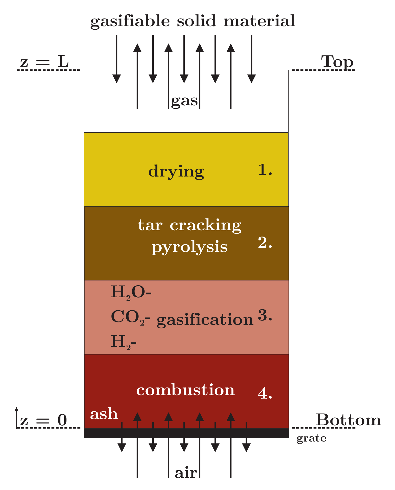
For stationary one-dimensional (1D) problems, the equations presented in Section 3 simplify to a set of ordinary differential equations (ODE) describing temperature, the mass fraction of N₂, O₂, CO₂, CO, H₂O, H₂ and CH₄ and tar for the gas-phase and temperature, wood, wood-char and ash for the solid-phase. The spatial z-coordinate (Figure 1) is then the independent variable. The gas-phase equations are coupled with the solid-phase equations by the source terms described in Section 3; additional coupling is provided by the relationships describing the bed-structure. Since the gaseous gasification agent enters the gasifier at the bottom, while the wood-pellets are supplied at the top, that gasifier operates in a counter-current mode. Thus, the inlet conditions for the gasification agent are known at the bottom, while the inlet conditions for the wood-pellets are specified at the top. When ODEs are required to satisfy boundary (inlet) conditions at more than one value of the independent variable (z-coordinate), the resulting mathematical problem is called a two-point boundary value problem. Hobbs et al. [23] named such a situation as “a split boundary value problem” and developed an elaborative iterative procedure to satisfy the temperature boundary conditions at the top and bottom of the gasifier. Di Blasi [17] used a first-order Euler method to solve the ODEs; no information was given on how the boundary conditions were handled. Mandl et al. [24] used a two-step iterative method; in the first step, guessed values were used for the unknown boundary conditions at the top where the integration begun and proceeded downwards using an explicit Runge-Kutta [60] procedure. In the second step, the unknown (guessed) boundary conditions were varied using the secant method [60] to match the boundary conditions at the bottom. The method, often called shooting, is inherently unstable, and good initial guesses are the secret to convergence.

In this paper, we present a novel method of handling the 1D two-point boundary value problem of counter-current gasification. The method is simple and eliminates mathematical difficulties associated with conventional solvers. Figure 4 shows an organigram of the method. In the first initialization step, the gas-phase temperature and mass fractions of N₂, O₂, CO₂, CO, H₂O, H₂and CH₄ are given values (for all values of z-coordinate) determined by the inlet (bottom) conditions; the solid-phase temperature and mass fractions of water-vapour, volatiles, char and ash are initialized with the top inlet values. After initialization, the gas-phase ODEs are solved upwards, beginning at the bottom, using the multi-step solver (MATLAB^®, ode15s) for stiff equations. During the integration of the gas-phase equations, the solid-phase variables remain frozen. Now all the source terms are evaluated (step 4 in Figure 4); no linearization is required. Then the solid-phase ODEs are solved downwards, from the top to the bottom, using the same solver (MATLAB^®, ode15s). During this integration, the gas-phase variables remain frozen. Then, again, the source-terms are evaluated (step 6 in Figure 4). The procedure is terminated when the following convergence criteria are satisfied:

-

for the mass fraction of all gas-phase and solid-phase components

$$|w_i^k-w_i^{k+1}|<0.0001$$

-

for gas-phase and solid-phase temperatures

$$|T^k-T^{k+1}|<0.01K$$

where indices k and $k+1$ indicate two consecutive iterations (an iteration includes a solution of the gas-phase ODEs upwards and subsequent solution of the solid-phase ODEs downwards). The above criteria have to be satisfied at all numerical divisions (grid points) in the z-coordinate. After a converged solution is found, both the overall mass and energy balances are checked. In all calculations presented here, the mass and energy balances are closed with an accuracy of ${10}^{-2}$–${10}^{-4}$ of the inlet values.

For the 3D version of the model described in Section 3, the CFD solver ANSYS^® FLUENT (version 17.1) for porous-beds is used. The problem of how to impose appropriate boundary conditions, at the bottom and at the top, still remains. Figure 5 shows the organigram of the solution procedure; the essence is the use of two instances of the CFD solver run in parallel. The first instance solves the gas-phase equations only, after which the sources are evaluated and passed on to the second instance, which solves the solid-phase equations. The communication between the two instances, facilitated every 25 iterations, is provided by the User-Defined Functions. The same 3D numerical grid is used for both instances. The procedure is terminated when the above convergence criteria are satisfied.

We wish to finish this Section with a remark. The above-described 1D and 3D procedures for computing of the counter-current reactor are used for steady-state calculations. We are sure that the same procedures can be used in time-dependent computing.

5. Results

Predictions of both the 1D and 3D versions of the mathematical model described in Section 3 are considered here. The predictions correspond to the experimental run of Mandl et al. [24] so that the boundary and inlet conditions listed in

Table 5. Boundary conditions for the 1D- and 3D-simulations.

	1D-Model	3D-Model
solid-phase inlet
wood-pellets
mass flow rate (kg/h)	3.5	3.5
${\rho }_{\mathrm{solid}}$ (kg/m³)	598	598
${\rho }_{\mathrm{char}}$ (kg/m³)	152.5	152.5
wood-pellets	moisture: 8%, ash: 0.4%,	moisture: 8%, ash: 0.4%,
composition (wt%)	char: 23.36%, volatiles: 68.24%	char: 23.36%, volatiles: 68.24%
temperature (K)	293	293
solid-phase outlet	-	pressure outlet
		(static pressure p = const)
gas-phase inlet
air-to-fuel ratio ($\frac{\mathrm{kg}}{\mathrm{kg}}$)	1.45	1.45
air composition (vol%)	${\mathrm{O}}_2$: 21%, $N_2$: 78.5%, ${\mathrm{H}}_2\mathrm{O}$: 0.5%	${\mathrm{O}}_2$: 21%, $N_2$: 78.5%, ${\mathrm{H}}_2\mathrm{O}$: 0.5%
temperature (K)	293	293
gas-phase outlet	-	pressure outlet
		(static pressure p = const)
wall temperature (K)	293	293
correction factor $\xi$ Equation (52)	1	1

are identical to Table 4 of Mandl et al. [24]. The gasifier’s diameter and height are 0.125 m and 0.42 m, respectively. Wood-pellets of a 0.0103 m equivalent diameter are gasified in a counter-current, steady-state operation. With a 3.5 kg/h wood-pellets supply rate and 17 MJ/kg Lower Calorific Value of the wood, the gasifier operates at 16.5 kW thermal input. The reactor was ignited introducing an ignition energy source in the middle of the reactor; the source ceased after 10 iterations.

Since the energy balances for the solid- and gas-phases are second-order differential equations, two additional boundary conditions must be specified for the upper and lower part of the counter-current gasifier, which are as follows [17,39]:

$$\frac{\partial T_g}{\partial z}=\frac{\partial T_s}{\partial z}=0$$

(63)

Extensive studies have been performed to obtain grid-independent numerical solutions. In 1D computing, 100, 1000, 2000 and 3000 divisions (along 0.42 m gasifier height) were tested, while in 3D computing, 63,360, 214,900 and 1,235,600 nodes were used. The 1D grid-independent results were obtained using 2000 nodes, while in the 3D grid-independent results, 214,900 nodes were used. Details of the sensitivity studies can be found in Schwabauer [20], see also Sosnowski et al. [61].

5.1. Comparison with the Measured Data

Figure 6 (Top) shows the measured and predicted temperatures of both the gas-phase and the solid-phase. The 1D and 3D predictions, both obtained with $\xi$ = 1, match each other very well, demonstrating the correctness of the method used for gas-phase/solid-phase coupling. In the 3D simulations, the heat-loss through the reactor walls is the only element that may bring 3D effects. Since the heat-loss is small, amounting to 4% of the fuel input (=16.58 kW), all dependent variables vary marginally with the gasifier radius. Thus, it is not too surprising that 1D and 3D predictions match well.

Differences between the predicted gas-phase and solid-phase temperatures are typically not larger than 50 K. The predicted temperatures match the measurements well, and the differences are typically not larger than 75 K; slightly larger values than measured are predicted at elevations above 0.1 m. The four zones, namely drying, pyrolysis, gasification and combustion, are also shown in Figure 6 (Top). Arbitrarily chosen criteria for their boundaries are as follows. The drying zone, beginning at z = 0.42 m, ends up when the moisture content of pellets is smaller than ${10}^{-4}$, while the pyrolysis zone ends when the mass fraction of the volatiles remaining in pellets is smaller than ${10}^{-5}$. The thickness of the oxidation zone corresponds to the z-coordinate at which the oxygen mass fraction in the gas-phase is smaller than ${10}^{-4}$. Indeed, the gasification zone is the largest, as one would expect, with gasification reactions proceeding with appreciable rates in the region where temperatures are larger than around 1000 K. The model predicts a rather thin pyrolysis zone as a consequence of the very fast pyrolysis rate.

Figure 6 (Bottom) shows TU Graz’s predictions (see Figure 5 in Mandl et al. [24]), which generally are of the same quality. It is important to realize that TU Graz’s predictions were obtained using different numerics and with a 0.5 value of the correction factor.

Figure 7 shows gas composition predictions using both 1D and 3D model versions. Again, both versions provide very similar values with the largest deviations occurring in CO predictions. This is attributed to slight differences in the gas-phase temperature predictions; carbon monoxide concentration-being temperature-dependent through the water gas-shift reaction-is then slightly altered. Both versions provide good predictions of the gas composition at the gasifier outlet, as shown in

Table 6. The producer-gas composition at the gasifier outlet.

Component	Measurements of Mandl et al. [24]	This Work	Model of Mandl et al. [24] without Adjustments	Model of Mandl et al. [24] with Adjustments
$\mathrm{C}\mathrm{O}$ vol%	22.6	21.8	21.4	22.9
$\mathrm{C}{\mathrm{O}}_2$ vol%	4.8	6.6	5.6	5.8
${\mathrm{H}}_2\mathrm{O}$ vol%	15.5	13.4	14.0	14.6
${\mathrm{H}}_2$ vol%	4.3	5.8	3.0	3.1
$\mathrm{C}{\mathrm{H}}_4$ vol%	2.7	1.6	0.8	2.1
$tar$ vol%	4.3	4.4	6.1	4.2
LCV MJ/Nm³	8.6	8.5	9.3	8.2
LCV MJ/kg	6.7	6.6	6.7	6.3
cold-gas efficiency $\eta$	89.1	87.3	90.3	83.6

. Cold-gas efficiency, listed in Table 6, is calculated as [19,62]

$${\eta }_{coldgasefficiency}=\frac{{\dot{m}}_{producergas}·{LCV}_{producergas}}{{\dot{m}}_{wood-pellets}·{LCV}_{wood-pellets}}$$

(64)

Table 6 also contains predictions of Mandl et al. [24] where under-predicted CO, H₂ and CH₄ $\mathrm{C}{\mathrm{H}}_4$ concentrations at the gasifier outlet (see Figure 6 in Mandl et al. [24]) are to be noticed. To remedy this shortcoming, the yield of the pyrolysis reaction was modified [24], and the improved predictions are shown in the fifth column of Table 6. No such adjustments were made in our simulations.

5.2. The Correction Factor

The correction factor $\xi$, appearing in Equation (46), was already introduced into the modelling in the 1980s and 1990s [18], so it is around forty years old. As shown in Equation (46), the factor governs the energy transfer between the gas- and solid-phases; for $\xi$ = 1, the rate is maximum, while for $\xi$ = 0, there is no energy transfer between the phases. Thus, with $\xi$ approaching 1, the differences between gas-phase and solid-phase temperatures are minimized. In all the previous works [17,18,24], the factor was used for tuning the temperature predictions to the measured values, and, due to imperfections of the numerical solvers (Section 4.2), obtaining stable and converged solutions was possible for some (selected) values of $\xi$ only. On the contrary, the solvers presented in Section 4.2 provide unconditionally stable and converged solutions for any $\xi$ values in the range zero to one.

Figure 8 demonstrates importance of $\xi$, showing both gas-phase and solid-phase temperatures for $\xi$= 1, $\xi$ = 0.5 (Mandl et al. [24]) and $\xi$ = 0.2 (Di Blasi [17]). The onset of the pyrolysis zone is a strong function of $\xi$, as shown in Figure 8.

Table 7. The influence of the correction factor $\xi$ on the predicted composition and LCV of the producer-gas as well as on cold-gas efficiency.

Producer Gas	Measurements of Mandl et al. [24]	This Work Equation (52) $\mathit{\xi }$ = 1	This Work Equation (52) $\mathit{\xi }$ = 0.5	This Work Equation (52) $\mathit{\xi }$ = 0.2
$\mathrm{C}{\mathrm{O}}_2$ vol%	4.8	6.6	6.24	7.6
$\mathrm{C}\mathrm{O}$ vol%	22.6	21.8	22.8	23.2
${\mathrm{H}}_2\mathrm{O}$ vol%	15.5	13.4	13.1	12.9
${\mathrm{H}}_2$ vol%	4.3	5.8	6.1	7.9
$\mathrm{C}{\mathrm{H}}_4$ vol%	2.7	1.6	2.0	4.2
$tar$ vol%	4.3	4.4	3.9	2.3
LCV MJ/Nm³	8.6	8.5	8.1	7.6
LCV MJ/kg	6.7	6.5	6.4	6.3
cold-gas efficiency	89.1	87.3	85.7	85.3

shows the dependence of $\xi$ on the predicted composition and LCV of the producer-gas.

5.3. Scaling

The small-scale (16.6 kW) gasifier of Mandl et al. [24] produced a low-BTU gas of 6.7 kJ/kg (LCV) with 89% cold gas efficiency (Table 6), which was indeed a good performance. Thus, the question of scaling the design to industrial-size is relevant.

Combustion system scaling is generally a complex procedure, particularly when flames are to be scaled [63]. However, for moving-bed reactors, the procedure is straight forward; the key parameters are the residence time of the solid-phase and the air-to-fuel ratio. According to the 1D predictions, the solid-phase remained in the reactor for 0.88 h.

Table 8. Parameters of the reactor series.

	Standard Case 1x	10x	25x	50x	100x	571x
Model Inputs
reactor height ( $\mathrm{m}$)	0.45	0.948	1.287	1.62	2.041	3.697
reactor diameter ( $\mathrm{m}$)	0.125	0.263	0.357	0.45	0.567	1.026
thermal power ( $\mathrm{k}$$\mathrm{W}$)	16.6	165.8	414	829	1658.6	9477
reactor height/	3.6	3.6	3.6	3.6	3.6	3.6
reactor diameter
reactor volume ( ${\mathrm{m}}^3$)	0.00515	0.0515	0.1288	0.2576	0.5153	2.945
side surface area ( $\mathrm{m}$)	0.57	1.6	2.56	3.70	5.42	15.14
residence time $\tau$ ( $\mathrm{h}$)	0.88	0.88	0.88	0.88	0.88	0.88
mass flow of	3.5	35	87.5	175	350	2000
the feedstock ( $\mathrm{k}$$\mathrm{g}$/ $\mathrm{h}$)
density of	598	598	598	598	598	598
the feedstock ( $\mathrm{k}$$\mathrm{g}$/ ${\mathrm{m}}^3$)
air volume flow	0.00585	0.0585	0.1463	0.2926	0.5853	3.344
in ( ${\mathrm{m}}^3$/ $\mathrm{h}$)
Predictions
outlet solid-phase	1360	1389	1653	1700	1744	1833
temperature ( $\mathrm{K}$)
outlet gas-phase	441	557	598	605	633	645
temperature ( $\mathrm{K}$)
producer-gas	6.6	6.4	6.4	6.4	6.4	6.3
calorific value ( $\mathrm{k}$$\mathrm{J}$/ $\mathrm{k}$$\mathrm{g}$)
cold-gas	87	85	85	85	85	84
efficiency (%)
heat losses ( $\mathrm{k}$$\mathrm{W}$)	0.65	2.5	4.5	7.7	12.6	50

shows a series of gasifiers for which the solid-phase residence time is kept at 0.88 h, and the air-to-fuel ratio is 1.45. The smallest thermal input of 16.6 kW (standard case in Table 8) corresponds to Mandl et al. [24] experiments, while the largest input is 9.5 MW with four scales between. All the gasifiers remain in geometrical proportions since the height-to-diameter ratio remains at 3.6 so that the velocity of gasification air remains the same. At each scale, wood-pellets of the same composition and size are used.

It is seen in Table 8 that the calorific value of the producer-gas tends to decrease with increasing input, while the cold-gas efficiency decreases from 87% for 16.6 kW input to 84% for the 9.5 MW scale [20]. Figure 9 shows a substantial increase of both solid-phase and gas-phase temperatures with the reactor size. This is attributed to the reduction of heat loss with the increased size. The heat loss amounts to around 4% of 16.6 kW thermal input, while at 9.5 MW, 0.5% heat loss is applicable. In other words, the effect of the surface/volume ratio of the reactor is clearly visible. Since the exit temperatures increase with thermal input, the cold-gas efficiency decreases accordingly. The predictions show that only ash leaves the reactor bottom so that the full conversion of the wood-pellets is observed at all scales.

Table 9. Producer-gas composition for different gasifier sizes.

	1x	10x	25x	50x	100x	571x
gas-phase
$\mathrm{C}{\mathrm{O}}_2$ (mol%)	6.6	5.0	4.8	4.7	4.6	4.5
$\mathrm{C}\mathrm{O}$ (mol%)	21.8	24.0	24.6	24.8	25.1	25.3
${\mathrm{H}}_2\mathrm{O}$ (mol%)	13.4	14.2	14.3	14.4	14.5	14.6
${\mathrm{H}}_2$ (mol%)	5.4	4.4	4.3	4.2	4.1	4.10
$\mathrm{C}{\mathrm{H}}_4$ (mol%)	1.6	1.8	2.0	2.1	2.2	2.4
tars (mol%)	4.4	4.1	4.0	3.9	3.8	3.7
solid-phase
volatiles (mass%)	0	0	0	0	0	0
char (mass%)	0	0	0	0	0	0
water (mass%)	0	0	0	0	0	0

and Figure 10 show the influence of scale on the gas composition. At all scales, CO, CO₂ and H₂O are formed in the combustion zone; CO₂, H₂O and H₂ are then consumed in the gasification reactions. The 6.5% CO₂ concentration in the producer-gas, observed at the 16.6 kW scale, drops to approximately 4.5% at 9.5 MW, while CO increases from 21.8% to 25.3%. The tar concentration is reduced from 4.4% to approximately 3.7% with increasing the scale, which is desirable. As described above, the calorific value of the producer-gas decreases slightly with scale [20].

In the above-described gasifier scaling, we have computed both the gas-phase and solid-phase temperatures as well as gas-phase composition along with the gasifier height. Table 8 lists the predicted gas-phase temperature and the calorific value of the producer-gas at the gasifier outlet for the six scales considered. A question is which of these two gasifier exit parameters (gas temperature or calorific value) has been predicted with a larger confidence? In light of the relatively close agreement (shown in Figure 6) between the measured and predicted temperatures, one may expect that the local heat-release rates have been correctly predicted for all the scales considered. Since the heat losses constitute a rather small fraction (see above) of the thermal input, we place a larger confidence on the temperature predictions than on the calorific value predictions.

6. Conclusions

The essence of this paper is the steady-state mathematical model of a moving-bed reactor for gasification of wood-pellets in air. Two versions of the model have been developed to simulate counter-current operation: the one-dimensional (1D) version-solving a set of Ordinary Differential Equations along the gasifier height-and the three-dimensional (3D) version where the balanced equations are solved using Computational Fluid Dynamics used separately for the gas-phase and solid-phase equations. Unique procedures were developed to provide unconditionally stable solutions and remove difficulties occurring from conventional numerical methods [17,18,23,24] in modelling counter-current reactors. The procedures reduce the uncertainties introduced by other mathematical approaches, and they open up the possibility of a straightforward application to more complex software, including commercial CFD packages.

Mandl et al. [24] describe both experiments and 1D mathematical modelling of the small-scale (16.6 kW) gasifier of wood-pellets. Their mathematical model contains a correction factor, appearing also in previous publications [17,18], which was used to tune the temperature predictions to the measured values. It has been demonstrated in this paper that the factor is not required.

The 16.6 kW gasifier of Mandl et al. [24], producing a low-BTU gas of LCV = 6.6 MJ/kg, operates at 89% cold-gas efficiency, which is indeed a good performance. Using the 1D model, the performance of a series of scaled versions of the reactor was examined, with the largest size of 9.5 MW. Calculations indicate a slight decrease of the producer-gas LCV from 6.6 MJ/kg (at 16.6 kW) to 6.3 MJ/kg (at 9.5 MW). The cold-gas efficiency decreases slightly from 89% to 84%, confirming the attractiveness of the design.

Mandl et al. [24] and Di Blasi [17] models, as well as the model presented in this paper, contain a large number of kinetic data, all taken from the literature. Now, after the uncertainties in the numerical solver have been removed, there is a need to examine the sensitivity of the models to the kinetics used.

References

1. Leckner, B. Co-combustion: A summary of technology. Therm. Sci. 2007, 4, 5–40. [Google Scholar] [CrossRef]
2. Williams, A.; Pourkashanian, M.; Jones, J. The combustion of coal and some other solid fuels. Proc. Combust. Inst. 2000, 28, 2141–2162. [Google Scholar] [CrossRef]
3. Weber, R.; Poyraz, Y.; Beckmann, A.M.; Brinker, S. Combustion of biomass in jet flames. Proc. Combust. Inst. 2015, 35, 2749–2758. [Google Scholar] [CrossRef]
4. Bashir, M.S.; Jensen, P.A.; Frandsen, F.; Wedel, S.; Dam-Johansen, K.; Wadenbäck, J.; Pedersen, S.T. Suspension-Firing of Biomass. Part 1: Full-Scale Measurements of Ash Deposit Build-up. Energy Fuels 2012, 26, 2317–2330. [Google Scholar] [CrossRef] [Green Version]
5. Hansen, S.B.; Jensen, P.A.; Frandsen, F.J.; Wu, H.; Bashir, M.S.; Wadenbäck, J.; Sander, B.; Glarborg, P. Deposit Probe Measurements in Large Biomass-Fired Grate Boilers and Pulverized-Fuel Boilers. Energy Fuels 2014, 28, 3539–3555. [Google Scholar] [CrossRef]
6. Hupa, M.; Karlström, O.; Vainio, E. Biomass combustion technology development – It is all about chemical details. Proc. Combust. Inst. 2017, 36, 113–134. [Google Scholar] [CrossRef]
7. Weber, R.; Poyraz, Y.; Mancini, M.; Schwabauer, A. Biomass Fly-Ash Deposition: Dependence of Deposition Rate on Probe/Particle Temperature in 115–1200 °C Range. Fuel 2021, 290, 120033. [Google Scholar] [CrossRef]
8. Bridgwater, A. Renewable fuels and chemicals by thermal processing of biomass. Chem. Eng. J. 2003, 91, 87–102. [Google Scholar] [CrossRef]
9. Scholz, R.; Beckmann, M.; Pieper, C.; Muster, M.; Weber, R. Considerations on providing the energy needs using exclusively renewable sources: Energiewende in Germany. Renew. Sustain. Energy Rev. 2014, 35, 109–125. [Google Scholar] [CrossRef]
10. Gŏmez-Barea, A.; Leckner, B. Modeling of biomass gasification in fluidized bed. Prog. Energy Combust. Sci. 2010, 36, 444–509. [Google Scholar] [CrossRef]
11. Higman, C. 5—Gasification process technology. In Advances in Clean Hydrocarbon Fuel Processing; Khan, M.R., Ed.; Woodhead Publishing Series in Energy; Woodhead Publishing: Sawston, UK, 2011; pp. 155–185. [Google Scholar] [CrossRef]
12. Chopra, S.; Jain, A.K. A Review of Fixed Bed Gasification Systems for Biomass. Agric. Eng. Int. Cigr J. 2007, 9. [Google Scholar]
13. Eberhard, M.; Santo, U.; Michelfelder, B.; Günther, A.; Weigand, P.; Matthes, J.; Waibel, P.; Hagenmeyer, V.; Kolb, T. The bioliq® Entrained-Flow Gasifier—A Model for the German Energiewende. ChemBioEng Rev. 2020, 7, 106–118. [Google Scholar] [CrossRef]
14. Kolb, T.; Aigner, M.; Kneer, R.; Müller, M.; Weber, R.; Djordjevic, N. Tackling the challenges in modelling entrained-flow gasification of low-grade feedstock. J. Energy Inst. 2016, 89, 485–503. [Google Scholar] [CrossRef] [Green Version]
15. Safronov, D.; Förster, T.; Schwitalla, D.; Nikrityuk, P.; Guhl, S.; Richter, A.; Meyer, B. Numerical study on entrained-flow gasification performance using combined slag model and experimental characterization of slag properties. Fuel Process. Technol. 2017, 161, 62–75. [Google Scholar] [CrossRef]
16. Möller, R. Synthesegasherstellung aus Kunststoffabfällen—Erfahrungen und Kennzahlen aus der Inbetriebnahme einer 32 MW-Pilotanlage; Thomé-Kozmiensky, K.J., Beckmann, M., Eds.; Chapter Alternativen zur Abfallverbrennung; TK Veriag: Neuruppin, Germany, 2014; Volume 11, pp. 797–808. [Google Scholar]
17. Di Blasi, C. Modeling wood gasification in a countercurrent fixed-bed reactor. AIChE J. 2004, 50, 2306–2319. [Google Scholar] [CrossRef] [Green Version]
18. Hobbs, M.L.; Radulovic, P.; Smoot, L.D. Combustion and Gasification of Coal in Fixed-Beds. Prog. Energy Combust. Sci. 1993, 19, 505–586. [Google Scholar] [CrossRef]
19. Higman, C.; van der Burgt, M. Gasification; Gulf Professional Publishing: Burlington, MA, USA, 2003. [Google Scholar] [CrossRef]
20. Schwabauer, A. Modellierung eines Wanderbett-Gegenstromvergasers. Ph.D. Thesis, Technische Universität Clausthal, Clausthal-Zellerfeld, Germany, 2019. [Google Scholar]
21. Mahishi, M.R.; Goswami, D. Thermodynamic optimization of biomass gasifier for hydrogen production. Int. J. Hydrog. Energy 2007, 32, 3831–3840. [Google Scholar] [CrossRef]
22. Shabbar, S.; Janajreh, I. Thermodynamic equilibrium analysis of coal gasification using Gibbs energy minimization method. Energy Convers. Manag. 2013, 65, 755–763. [Google Scholar] [CrossRef]
23. Hobbs, M.L.; Radulovic, P.T.; Smoot, L.D. Modeling fixed-bed coal gasifiers. AIChE J. 1992, 38, 681–702. [Google Scholar] [CrossRef]
24. Mandl, C.; Obernberger, I.; Biedermann, F. Modelling of an updraft fixed-bed gasifier operated with softwood pellets. Fuel 2010, 89, 3795–3806. [Google Scholar] [CrossRef]
25. Mikulandrić, R.; Lončar, D.; Böhning, D.; Böhme, R.; Beckmann, M. Artificial neural network modelling approach for a biomass gasification process in fixed bed gasifiers. Energy Convers. Manag. 2014, 87, 1210–1223. [Google Scholar] [CrossRef]
26. Yang, Y.; Goh, Y.; Zakaria, R.; Nasserzadeh, V.; Swithenbank, J. Mathematical modelling of MSW incineration on a travelling bed. Waste Manag. 2002, 22, 369–380. [Google Scholar] [CrossRef]
27. Hermansson, S.; Thunman, H. CFD modelling of bed shrinkage and channelling in fixed-bed combustion. Combust. Flame 2011, 158, 988–999. [Google Scholar] [CrossRef]
28. Sharma, A.K. Modeling and simulation of a downdraft biomass gasifier 1. Model development and validation. Energy Convers. Manag. 2011, 52, 1386–1396. [Google Scholar] [CrossRef]
29. Jaojaruek, K. Mathematical model to predict temperature profile and air–fuel equivalence ratio of a downdraft gasification process. Energy Convers. Manag. 2014, 83, 223–231. [Google Scholar] [CrossRef]
30. Janajreh, I.; Al Shrah, M. Numerical and experimental investigation of downdraft gasification of wood chips. Energy Convers. Manag. 2013, 65, 783–792. [Google Scholar] [CrossRef]
31. Yang, Y.B.; Ryu, C.; Khor, A.; Yates, N.E.; Sharifi, V.N.; Swithenbank, J. Effect of fuel properties on biomass combustion. Part II. Modelling approach—Identification of the controlling factors. Fuel 2005, 84, 2116–2130. [Google Scholar] [CrossRef]
32. González, W.A.; Pérez, J.F.; Chapela, S.; Porteiro, J. Numerical analysis of wood biomass packing factor in a fixed-bed gasification process. Renew. Energy 2018, 121, 579–589. [Google Scholar] [CrossRef]
33. Weber, R.; Gupta, A.K.; Mochida, S. High temperature air combustion (HiTAC): How it all started for applications in industrial furnaces and future prospects. Appl. Energy 2020, 278, 115551. [Google Scholar] [CrossRef]
34. Yang, W.; Ponzio, A.; Lucas, C.; Blasiak, W. Performance analysis of a fixed-bed biomass gasifier using high-temperature air. Fuel Process. Technol. 2006, 87, 235–245. [Google Scholar] [CrossRef]
35. Buczyński, R.; Weber, R.; Szlek, A.; Nosek, R. Time-Dependent Combustion of Solid Fuels in a Fixed-Bed: Measurements and Mathematical Modeling. Energy Fuels 2012, 26, 4767–4774. [Google Scholar] [CrossRef]
36. Grønli, M. Theoretical and Experimental Study of the Thermal Degradation of Biomass. Ph.D. Dissertation, NTNU, Trondheim, Norway, 1996. [Google Scholar]
37. Groeneveld, M.J.; van Swaaij, W. 39 Gasification of char particles with CO2 and H2O. Chem. Eng. Sci. 1980, 35, 307–313. [Google Scholar] [CrossRef] [Green Version]
38. Kashiwagi, T.; Nambu, H. Global kinetic constants for thermal oxidative degradation of a cellulosic paper. Combust. Flame 1992, 88, 345–368. [Google Scholar] [CrossRef]
39. Cooper, J.; Hallett, W. A Numerical Model for Packed-Bed Combustion of Char Particles. Chem. Eng. Sci. 2000, 55, 4451–4460. [Google Scholar] [CrossRef]
40. Bryden, K.; Ragland, K. Numerical Modeling of a Deep, Fixed-Bed Combustor. Energy Fuels 1996, 10, 269–275. [Google Scholar] [CrossRef]
41. Biba, V.; Macak, J.; Malecha, J.; Klose, E. Mathematical Model for the Gasification of Coal under Pressure. Ind. Eng. Chem. Process. Des. Dev. 1978, 17, 92–98. [Google Scholar]
42. Goldman, J.; Xieu, D.; Oko, A.; Milne, R.; Essenhigh, R.H. A comparison of prediction and experiment in the gasification of anthracite in air and oxygen-enriched steam mixtures. Symp. (Int.) Combust. 1985, 20, 1365–1372. [Google Scholar] [CrossRef]
43. Modest, M.F. Radiative Heat Transfer; Elsevier: Amsterdam, The Netherlands, 2013. [Google Scholar]
44. Arthur, J.R. Reactions between carbon and oxygen. Trans. Faraday Soc. 1951, 47, 164–178. [Google Scholar] [CrossRef]
45. Yoon, H.; Wei, J.; Denn, M.M. A model for moving-bed coal gasification reactors. AIChE J. 1978, 24. [Google Scholar] [CrossRef]
46. Radulovic, P.T.; Ghani, M.; Smoot, L. An improved model for fixed bed coal combustion and gasification. Fuel 1995, 74, 582–594. [Google Scholar] [CrossRef]
47. Aerts, P.D.; Ragland, K. Pressurized downdraft combustion of woodchips. Symp. (Int.) Combust. 1991, 23, 1025–1032. [Google Scholar] [CrossRef]
48. Verein Deutscher Ingenieure. VDI-Wärmeatlas; Auflage, Springer: Berlin/Heidelberg, Germany, 2013; Volume 11. [Google Scholar] [CrossRef]
49. Raznjevic, K. Handbook of Thermodynamic Tables and Charts; McGraw Hill: New York, NY, USA, 1976. [Google Scholar]
50. Roberts, A.; Clough, G. Thermal decomposition of wood in an inert atmosphere. Symp. (Int.) Combust. 1963, 9, 158–166. [Google Scholar] [CrossRef]
51. Glaister, D.S. The Prediction of Chemical Kinetic, Heat, and Mass Transfer Processes During the One-and Two-dimensional Pyrolysis of a Large Wood Pellet. Master’s Thesis, University of Washington, Seattle, DC, USA, 1987. [Google Scholar]
52. Liden, A.; Berruti, F.; Scott, D. A Kinetic Model for the Production of Liquids from the Flash Pyrolysis of Biomass. Chem. Eng. Commun. 1988, 65, 207–221. [Google Scholar] [CrossRef]
53. Weber, R. Extracting mathematically exact kinetic parameters from experimental data on combustion and pyrolysis of solid fuels. J. Energy Inst. 2008, 81, 226–233. [Google Scholar] [CrossRef]
54. Nowak, B.; Karlström, O.; Backman, P.; Brink, A.; Zevenhoven, M.; Voglsam, S.; Winter, F.; Hupa, M. Mass transfer limitation in thermogravimetry of biomass gasification. J. Therm. Anal. Calorim. 2013, 111, 182–192. [Google Scholar] [CrossRef]
55. Schulze, S.; Nikrityuk, P.; Abosteif, Z.; Guhl, S.; Richter, A.; Meyer, B. Heat and mass transfer within thermogravimetric analyser: From simulation to improved estimation of kinetic data for char gasification. Fuel 2017, 187, 338–348. [Google Scholar] [CrossRef]
56. Buczyński, R.; Czerski, G.; Zubek, K.; Weber, R.; Grzywacz, P. Evaluation of carbon dioxide gasification kinetics on the basis of non-isothermal measurements and CFD modelling of the thermogravimetric analyser. Fuel 2018, 228, 50–61. [Google Scholar] [CrossRef]
57. Wang, C.; Jin, H.; Feng, H.; Wei, W.; Cao, C.; Cao, W. Study on gasification mechanism of biomass waste in supercritical water based on product distribution. Int. J. Hydrog. Energy 2020, 45, 28051–28061. [Google Scholar] [CrossRef]
58. Nowicki, L.; Siuta, D.; Markowski, M. Carbon Dioxide Gasification Kinetics of Char from Rapeseed Oil Press Cake. Energies 2020, 13, 2318. [Google Scholar] [CrossRef]
59. Nowicki, L.; Siuta, D.; Markowski, M. Pyrolysis of Rapeseed Oil Press Cake and Steam Gasification of Solid Residues. Energies 2020, 13, 4472. [Google Scholar] [CrossRef]
60. Press, W.H.; Teukolsky, S.; Vettering, W.; Flannery, B. Numerical Recipes. The Art of Scientific Computing; Cambridge University Press: Cambridge, MA, USA, 2007. [Google Scholar]
61. Sosnowski, M.; Krzywanski, J.; Scurek, R. A Fuzzy Logic Approach for the Reduction of Mesh-Induced Error in CFD Analysis: A Case Study of an Impinging Jet. Entropy 2019, 21, 1047. [Google Scholar] [CrossRef] [Green Version]
62. Basu, P. Biomass Gasification, Pyrolysis and Torrefaction, 2nd ed.; Academic Press: Boston, MA, USA, 2013; pp. 199–248. [Google Scholar] [CrossRef]
63. Weber, R.; Mancini, M. On Scaling and Mathematical Modelling of Large Scale Industrial Flames. J. Energy Inst. 2020, 93, 43–51. [Google Scholar] [CrossRef]
Figure 1. Counter-current gasification of solid material [19,20].
Energies 14 05840 g001
Figure 2. Sketch of the moving-bed counter-current gasifier [24].
Energies 14 05840 g002
Figure 3. Rates of pyrolysis (1/s) and tar cracking (1/s) used in modelling.
Energies 14 05840 g003
Figure 4. Solution procedure for gas-phase and solid-phase equations [20].
Energies 14 05840 g004
Figure 5. Solution procedure for the CFD Solver of gas-phase and solid-phase equations [20].
Energies 14 05840 g005
Figure 6. Comparison of the calculated and measured temperatures [24]. The error bars show an error range of 50 K. Plotted 3D temperatures are averaged over gasifier diameter. (Top) our predictions; (Bottom) Mandl et al. [24] predictions.
Energies 14 05840 g006
Figure 7. The predicted gas composition along the reactor height in 1D and 3D simulations. 3D predictions are averaged over the reactor diameter. Symbols indicate values measured at the gasifier outlet [24].
Energies 14 05840 g007
Figure 8. Influence of the correction factor ξ on the solid- and gas-phase temperatures (Top) ξ = 1, (Middle) ξ = 0.5 and (Bottom) ξ = 0.2. The moving pyrolysis zone is highlighted in red.
Energies 14 05840 g008
Figure 9. The influence of the gasifier size (thermal input) on both gas-phase and solid-phase exit temperatures for constant residence time scaling [20].
Energies 14 05840 g009
Figure 10. The influence of the gasifier size (thermal input) on the gas composition for constant residence time scaling [20].
Energies 14 05840 g010