
Impact of Wind and Solar Generation on the Italian Zonal Electricity Price


Abstract
:1. Introduction
2. Literature Review
3. Italian Electricity Market
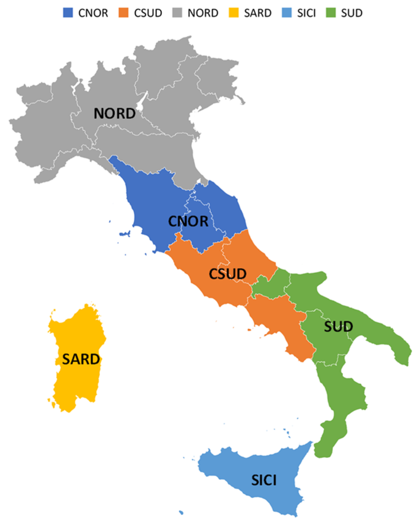
3.1. Introduction of the Italian Electricity Market
3.2. Price Formation Mechanism
3.3. Descriptive Statistics
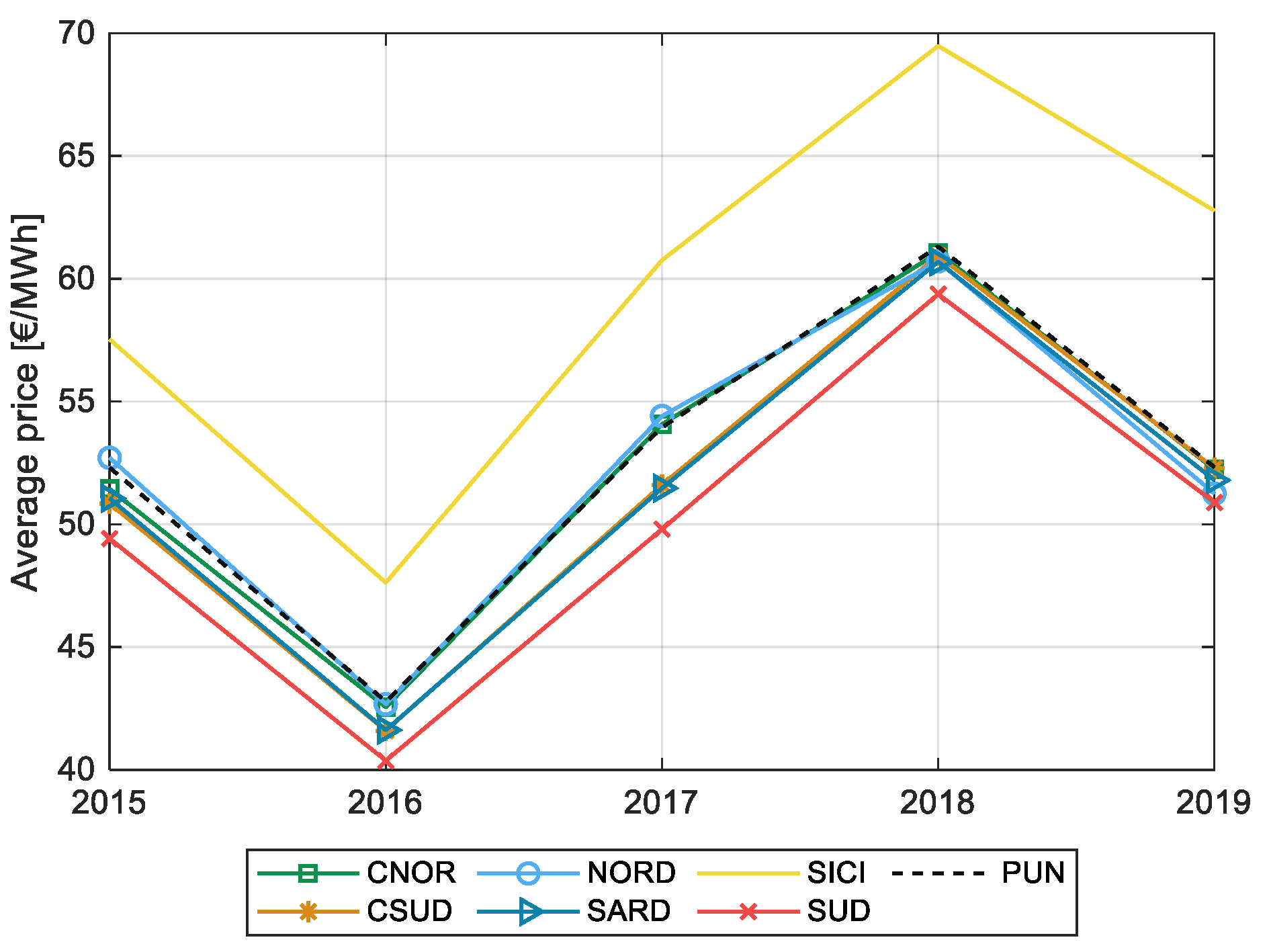
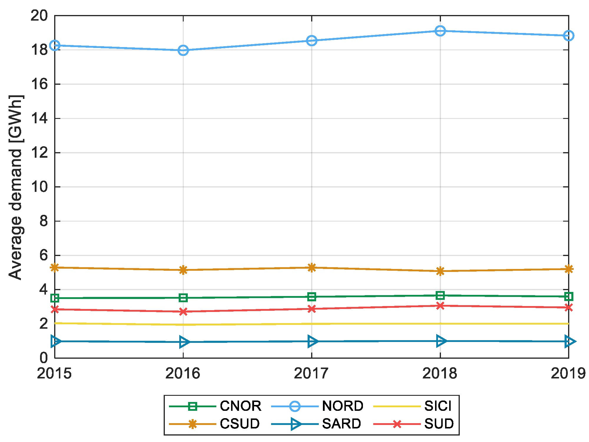
3.3.1. Zonal Price and Demand
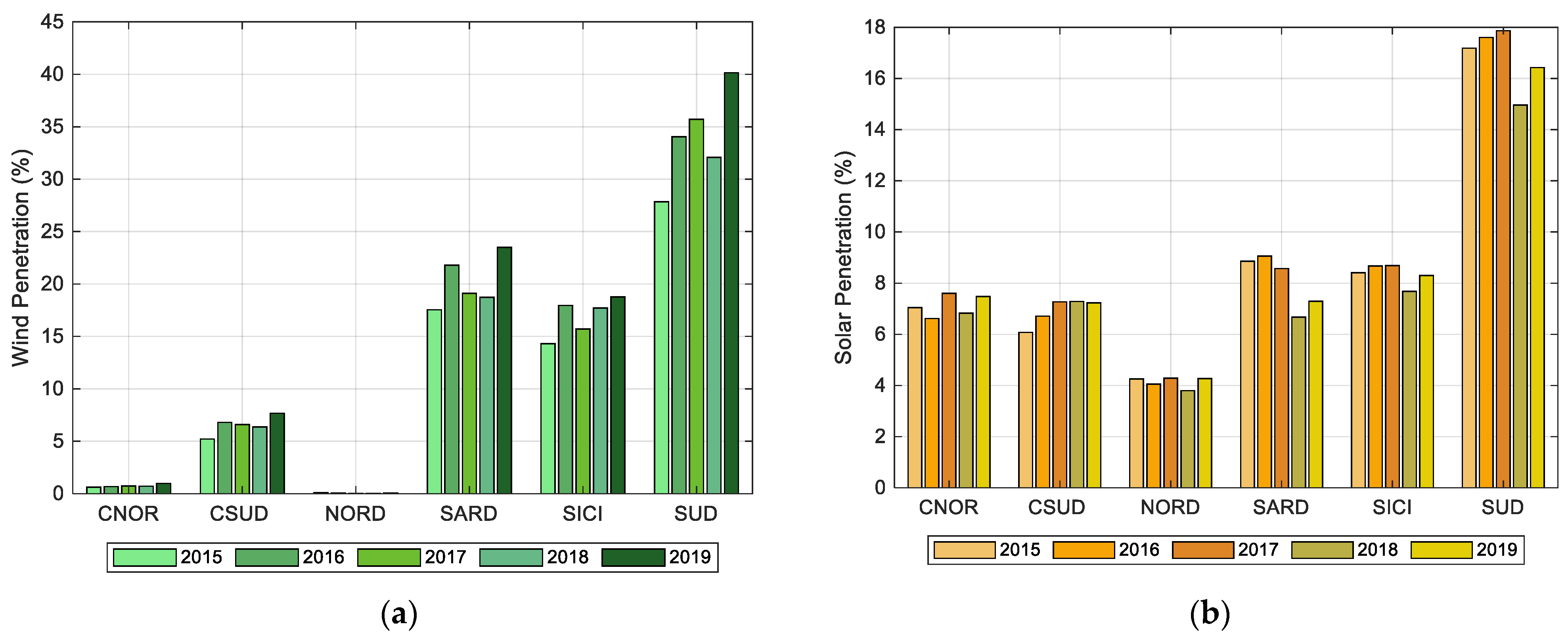
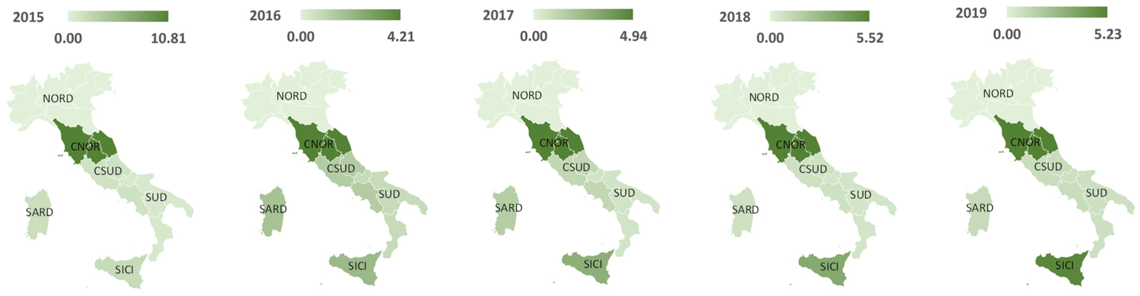
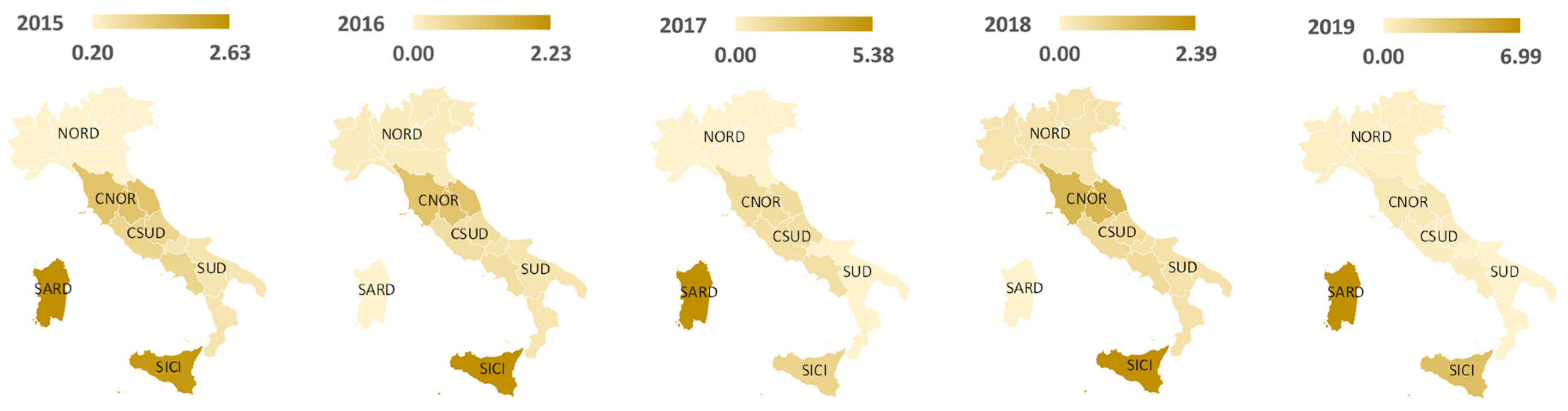
3.3.2. Wind and Solar Penetration
4. Methodology and Data
4.1. Preliminary Test
4.1.1. Augmented Dickey–Fuller Test
4.1.2. Variance Inflator Indicator
4.2. Multivariate Regression Model
- ➢
- First estimation: Estimating the impact of wind and solar generation on the net input flow of the given zone.
- ➢
- Second estimation: Estimating the impact of the wind and solar generation on the net input flow of the other zones.
- ➢
- Third estimation: Estimating the impact of wind and solar generation on the electricity price in the given zone.
4.3. Post-Processing
4.3.1. Breusch–Pagan Test
4.3.2. Durbin–Watson Test
5. Results
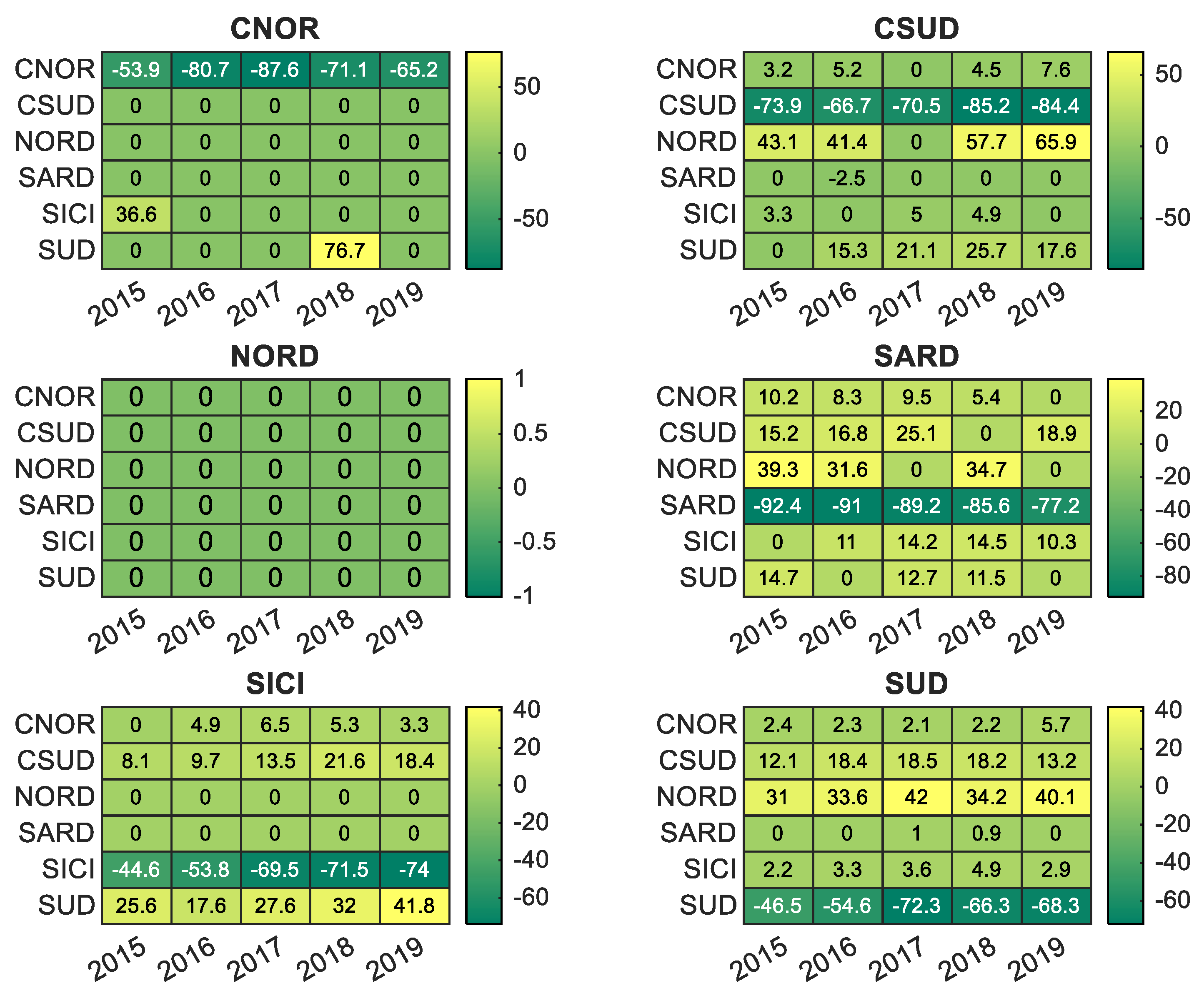
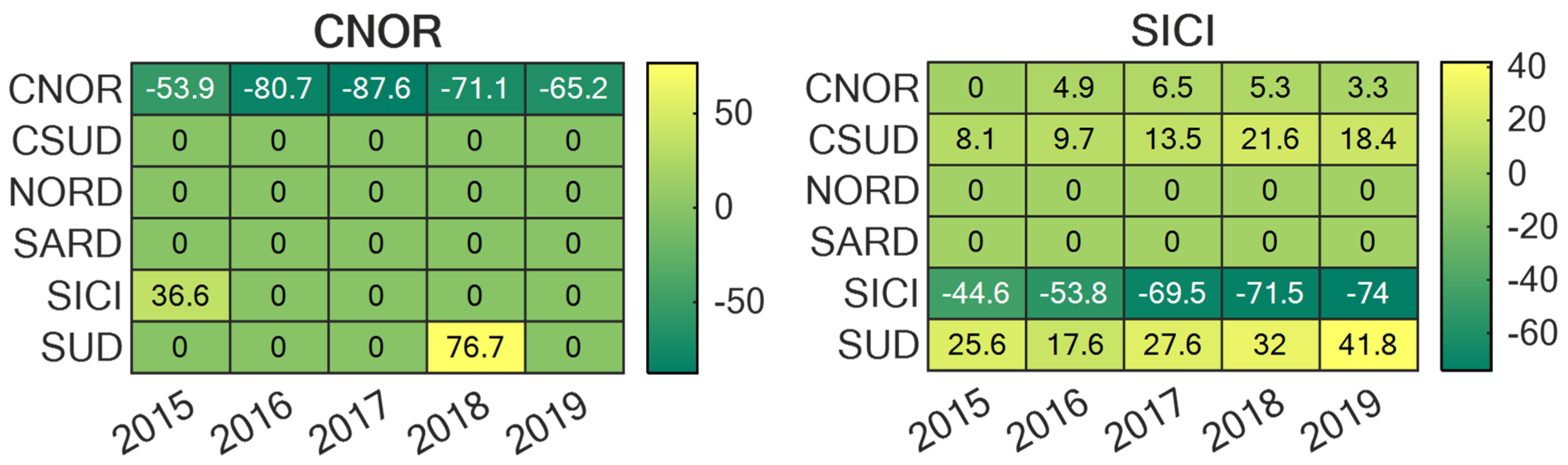
5.1. Impact of Wind and Solar Generation on the Net Input Flow of Each Zone
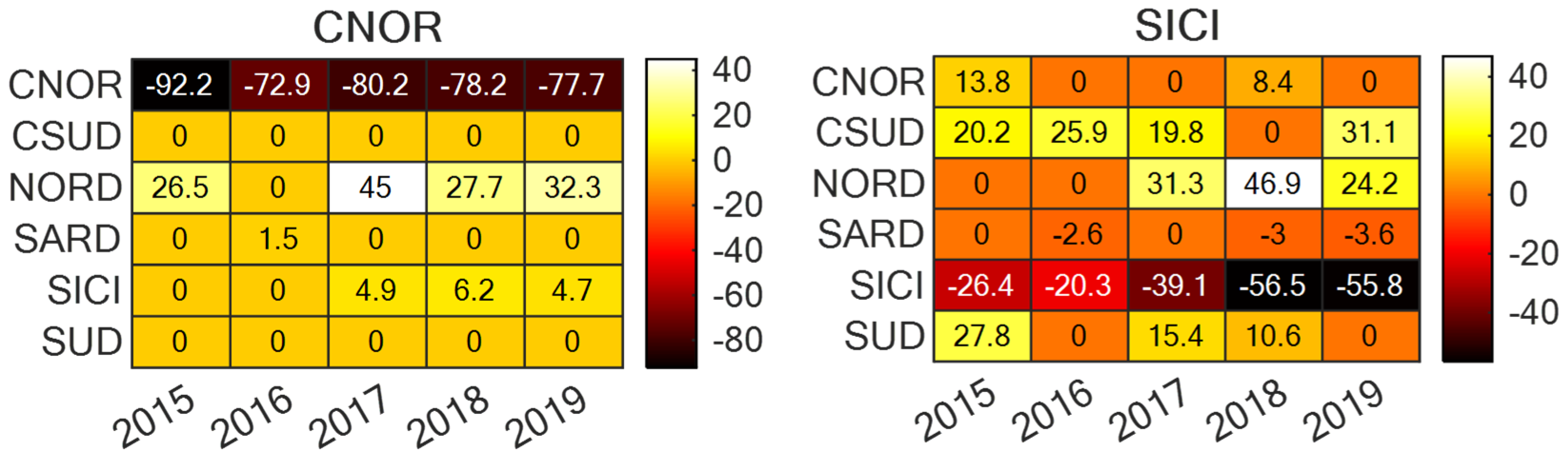
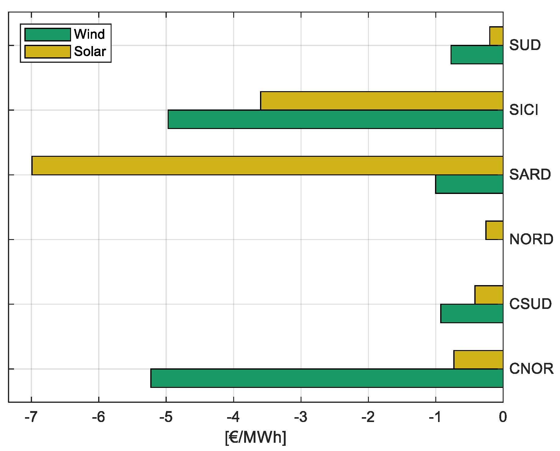
5.2. Impact of Wind and Solar Generation on the Zonal Market Price
6. Conclusions
Author Contributions
Funding
Conflicts of Interest
Appendix A

| CNOR | Input Variables | 2015 | 2016 | 2017 | 2018 | 2019 |
| ΔWind | −11.54 | −11.84 | −10.31 | −10.67 | −10.93 | |
| ΔSolar | −11.48 | −10.25 | −10.82 | −8.73 | −12 | |
| ΔDemand | −7.73 | −7.84 | −6.78 | −7.43 | −8.04 | |
| ΔNetIn | −7.95 | −9.41 | −8.16 | −8.75 | −7.97 | |
| ΔNetInother zones | −7.64 | −7.94 | −8.25 | −8.93 | −8.06 | |
| ΔNGPrice | −7.97 | −4.49 | −8.04 | −8.34 | −6.52 | |
| ΔZonalPrice | −9.45 | −8.73 | −7.51 | −7.08 | −8.1 |
| CSUD | Input Variables | 2015 | 2016 | 2017 | 2018 | 2019 |
| ΔWind | −11.11 | −11.21 | −10.52 | −10.91 | −12.23 | |
| ΔSolar | −11.76 | −10.03 | −10.98 | −8.69 | −11.74 | |
| ΔDemand | −6.89 | −7.12 | −7.09 | −6.93 | −8.25 | |
| ΔNetIn | −8.5 | −9.85 | −8.77 | −9 | −8.39 | |
| ΔNetInother zones | −7.44 | −7.75 | −8.5 | −8.79 | −8.05 | |
| ΔNGPrice | −7.97 | −4.49 | −8.04 | −8.34 | −6.52 | |
| ΔZonalPrice | −9.63 | −9.26 | −8.91 | −7.45 | −8.76 |
| NORD | Input Variables | 2015 | 2016 | 2017 | 2018 | 2019 |
| ΔWind | −9.87 | −10.36 | −9.49 | −9.98 | −11.51 | |
| ΔSolar | −11.15 | −11.49 | −11.57 | −9.48 | −12.37 | |
| ΔDemand | −7.72 | −7.27 | −6.56 | −7.3 | −7.44 | |
| ΔNetIn | −7.77 | −7.5 | −8.26 | −8.84 | −7.91 | |
| ΔNetInother zones | −8.4 | −9.05 | −9.22 | −8.93 | −9.82 | |
| ΔNGPrice | −7.97 | −4.49 | −8.04 | −8.34 | −6.52 | |
| ΔZonalPrice | −8.37 | −8.39 | −7.26 | −7.25 | −7.83 |
| SARD | Input Variables | 2015 | 2016 | 2017 | 2018 | 2019 |
| ΔWind | −9.47 | −9.17 | −10.57 | −10.64 | −10.59 | |
| ΔSolar | −10.52 | −9.67 | −10.88 | −8.88 | −11.77 | |
| ΔDemand | −6.94 | −8.23 | −7.82 | −9.77 | −10.19 | |
| ΔNetIn | −9.12 | −9.79 | −10.43 | −9.48 | −9.58 | |
| ΔNetInother zones | −7.37 | −7.58 | −8.2 | −8.89 | −7.94 | |
| ΔNGPrice | −7.97 | −4.49 | −8.04 | −8.34 | −6.52 | |
| ΔZonalPrice | −9.52 | −9.34 | −9.04 | −7.66 | −9.08 |
| SICI | Input Variables | 2015 | 2016 | 2017 | 2018 | 2019 |
| ΔWind | −10.27 | −10.57 | −10.3 | −10.35 | −11.1 | |
| ΔSolar | −10.91 | −9.91 | −9.19 | −9.76 | −9.96 | |
| ΔDemand | −6.88 | −8.14 | −7.33 | −7.56 | −7.48 | |
| ΔNetIn | −9.14 | −9.17 | −8.67 | −8.59 | −8.95 | |
| ΔNetInother zones | −7.39 | −7.56 | −8.07 | −8.97 | −7.85 | |
| ΔNGPrice | −7.97 | −4.49 | −8.04 | −8.34 | −6.52 | |
| ΔZonalPrice | −11.3 | −9.9 | −9.26 | −9.17 | −9.4 |
| SUD | Input Variables | 2015 | 2016 | 2017 | 2018 | 2019 |
| ΔWind | −11.08 | −11.65 | −10.88 | −10.65 | −11.61 | |
| ΔSolar | −10.16 | −10.38 | −11.02 | −9.12 | −11.22 | |
| ΔDemand | −7.18 | −8.62 | −7.67 | −7.4 | −7.56 | |
| ΔNetIn | −9.06 | −10.51 | −10.01 | −9.45 | −9.63 | |
| ΔNetInother zones | −7.41 | −7.48 | −8.02 | −8.78 | −8.25 | |
| ΔNGPrice | −7.97 | −4.49 | −8.04 | −8.34 | −6.52 | |
| ΔZonalPrice | −10.33 | −9.41 | −9.04 | −7.91 | −9.8 |
| CNOR | 2015 | 2016 | 2017 | 2018 | 2019 |
|---|---|---|---|---|---|
| ΔWind | −0.5394 *** | −0.8065 *** | −0.8757 *** | −0.7107 *** | −0.652 *** |
| (0.1904) | (0.1443) | (0.1361) | (0.1337) | (0.1368) | |
| ΔSolar | −0.922 *** | −0.7291 *** | −0.8023 *** | −0.7821 *** | −0.7772 *** |
| (0.0215) | (0.0173) | (0.0211) | (0.0189) | (0.0237) | |
| ΔDemand | 0.7426 *** | 0.7553 *** | 0.7527 *** | 0.722 *** | 0.6984 *** |
| (0.0095) | (0.0091) | (0.0119) | (0.0103) | (0.0114) | |
| ΔWindother zones | 0.0322 *** | 0.0376 *** | 0.0324 *** | 0.0339 *** | 0.0538 *** |
| (0.0049) | (0.005) | (0.0042) | (0.0038) | (0.0044) | |
| ΔSolarother zones | 0.0297 *** | 0.0057 ** | 0.0112 *** | 0.0172 *** | 0.0314 *** |
| (0.0031) | (0.0025) | (0.003) | (0.0027) | (0.0034) | |
| ΔDemandother zones | −0.0083 *** | −0.01 *** | −0.01 *** | −0.0081 *** | −0.014 *** |
| (0.0013) | (0.0012) | (0.0015) | (0.0014) | (0.0015) | |
| Dummies | Yes | Yes | Yes | Yes | Yes |
| Observations | 8760 | 8784 | 8760 | 8760 | 8760 |
| Adjusted R2 | 0.83 | 0.80 | 0.82 | 0.82 | 0.72 |
| CSUD | 2015 | 2016 | 2017 | 2018 | 2019 |
|---|---|---|---|---|---|
| ΔWind | −0.7392 *** | −0.6666 *** | −0.7051 *** | −0.8523 *** | −0.8439 *** |
| (0.0467) | (0.0461) | (0.0492) | (0.0449) | (0.0394) | |
| ΔSolar | −0.7165 *** | −0.3944 *** | −0.5554 *** | −0.6527 *** | −0.6153 *** |
| (0.0363) | (0.0395) | (0.0401) | (0.0341) | (0.0342) | |
| ΔDemand | 0.5216 *** | 0.3175 *** | 0.4061 *** | 0.4624 *** | 0.522 *** |
| (0.013) | (0.0176) | (0.0207) | (0.0187) | (0.0201) | |
| ΔWindother zones | 0.1127 *** | 0.1641 *** | 0.178 *** | 0.1816 *** | 0.1418 *** |
| (0.0175) | (0.0196) | (0.0187) | (0.0166) | (0.0149) | |
| ΔSolarother zones | 0.1057 *** | 0.1031 *** | 0.0985 *** | 0.0734 *** | 0.0877 *** |
| (0.0069) | (0.0083) | (0.0086) | (0.0078) | (0.0072) | |
| ΔDemandother zones | −0.0397 *** | −0.0337 *** | −0.0496 *** | −0.062 *** | −0.0735 *** |
| (0.0026) | (0.0034) | (0.0039) | (0.0035) | (0.0037) | |
| Dummies | Yes | Yes | Yes | Yes | Yes |
| Observations | 8760 | 8784 | 8760 | 8760 | 8760 |
| Adjusted R2 | 0.30 | 0.19 | 0.19 | 0.23 | 0.23 |
| NORD | 2015 | 2016 | 2017 | 2018 | 2019 |
|---|---|---|---|---|---|
| ΔWind | −0.0609 | 0.6564 | −1.7329 | 1.9037 | 0.0691 |
| (2.4724) | (2.5645) | (2.6314) | (2.6719) | (1.8237) | |
| ΔSolar | −0.3928 *** | −0.288 *** | −0.5204 *** | −0.3959 *** | −0.3584 *** |
| (0.0302) | (0.0339) | (0.0336) | (0.0291) | (0.0285) | |
| ΔDemand | 0.2534 *** | 0.2074 *** | 0.2764 *** | 0.229 *** | 0.2019 *** |
| (0.0085) | (0.0094) | (0.0101) | (0.0092) | (0.0091) | |
| ΔWindother zones | 0.2897 *** | 0.3054 *** | 0.311 *** | 0.3237 *** | 0.3668 *** |
| (0.0358) | (0.0327) | (0.0288) | (0.0239) | (0.0223) | |
| ΔSolarother zones | 0.2032 *** | 0.1274 *** | 0.283 *** | 0.344 *** | 0.3548 *** |
| (0.0195) | (0.0208) | (0.0209) | (0.0183) | (0.0189) | |
| ΔDemandother zones | −0.345 *** | −0.3345 *** | −0.3765 *** | −0.3665 *** | −0.3415 *** |
| (0.0114) | (0.0133) | (0.0139) | (0.0129) | (0.0128) | |
| Dummies | Yes | Yes | Yes | Yes | Yes |
| Observations | 8760 | 8784 | 8760 | 8760 | 8760 |
| Adjusted R2 | 0.11 | 0.18 | 0.11 | 0.12 | 0.12 |
| SARD | 2015 | 2016 | 2017 | 2018 | 2019 |
|---|---|---|---|---|---|
| ΔWind | −0.9242 *** | −0.9105 *** | −0.8916 *** | −0.8558 *** | −0.7718 *** |
| (0.0162) | (0.0147) | (0.0157) | (0.0173) | (0.0162) | |
| ΔSolar | −0.7915 *** | −0.725 *** | −0.6461 *** | −0.6912 *** | −0.5943 *** |
| (0.0269) | (0.0263) | (0.0288) | (0.0328) | (0.0345) | |
| ΔDemand | 0.5505 *** | 0.6917 *** | 0.5798 *** | 0.5093 *** | 0.3195 *** |
| (0.017) | (0.0155) | (0.017) | (0.0162) | (0.0155) | |
| ΔWindother zones | −0.0001 | −0.0044 | 0.0071 ** | 0.0073 ** | −0.0028 |
| (0.0031) | (0.0029) | (0.0028) | (0.003) | (0.0029) | |
| ΔSolarother zones | −0.0028 ** | −0.0036 *** | −0.0053 *** | −0.0059 *** | −0.0082 *** |
| (0.0013) | (0.0013) | (0.0013) | (0.0014) | (0.0014) | |
| ΔDemandother zones | 0.002 *** | 0.0004 | 0.0015 *** | 0.0024 *** | 0.0055 *** |
| (0.0005) | (0.0004) | (0.0005) | (0.0005) | (0.0005) | |
| Dummies | Yes | Yes | Yes | Yes | Yes |
| Observations | 8760 | 8784 | 8760 | 8760 | 8760 |
| Adjusted R2 | 0.61 | 0.66 | 0.61 | 0.51 | 0.48 |
| SICI | 2015 | 2016 | 2017 | 2018 | 2019 |
|---|---|---|---|---|---|
| ΔWind | −0.4463 *** | −0.5383 *** | −0.6949 *** | −0.7151 *** | −0.74 *** |
| (0.0146) | (0.0183) | (0.0199) | (0.0166) | (0.0182) | |
| ΔSolar | −0.2639 *** | −0.2032 *** | −0.3915 *** | −0.5646 *** | −0.5576 *** |
| (0.0195) | (0.0262) | (0.0303) | (0.0252) | (0.029) | |
| ΔDemand | 0.0941 *** | 0.111 *** | 0.2949 *** | 0.377 *** | 0.3923 *** |
| (0.0103) | (0.013) | (0.0163) | (0.0145) | (0.0167) | |
| ΔWindother zones | 0.0268 *** | 0.0364 *** | 0.049 *** | 0.0585 *** | 0.0313 *** |
| (0.0045) | (0.006) | (0.006) | (0.0054) | (0.0051) | |
| ΔSolarother zones | 0.0083 *** | 0.0004 | 0.0126 *** | 0.0167 *** | 0.0169 *** |
| (0.0018) | (0.0024) | (0.0027) | (0.0023) | (0.0026) | |
| ΔDemandother zones | −0.0082 *** | −0.0052 *** | −0.0118 *** | −0.0109 *** | −0.0096 *** |
| (0.0007) | (0.0009) | (0.0011) | (0.001) | (0.0011) | |
| Dummies | Yes | Yes | Yes | Yes | Yes |
| Observations | 8760 | 8784 | 8760 | 8760 | 8760 |
| Adjusted R2 | 0.14 | 0.13 | 0.19 | 0.30 | 0.28 |
| SUD | 2015 | 2016 | 2017 | 2018 | 2019 |
|---|---|---|---|---|---|
| ΔWind | −0.4653 *** | −0.5463 *** | −0.7233 *** | −0.6626 *** | −0.6831 *** |
| (0.0241) | (0.0228) | (0.0204) | (0.019) | (0.0167) | |
| ΔSolar | −0.3889 *** | −0.3753 *** | −0.4072 *** | −0.4345 *** | −0.4228 *** |
| (0.0233) | (0.0217) | (0.0228) | (0.0214) | (0.0231) | |
| ΔDemand | 0.1062 *** | 0.1508 *** | 0.0914 *** | 0.1241 *** | −0.0142 |
| (0.0158) | (0.0171) | (0.0206) | (0.0184) | (0.0233) | |
| ΔWindother zones | 0.1663 *** | 0.1517 *** | 0.2248 *** | 0.2641 *** | 0.2567 *** |
| (0.0307) | (0.0289) | (0.028) | (0.0248) | (0.0251) | |
| ΔSolarother zones | 0.0571 *** | 0.0238 *** | 0.0329 *** | 0.0432 *** | 0.0503 *** |
| (0.0074) | (0.0073) | (0.0072) | (0.0067) | (0.007) | |
| ΔDemandother zones | −0.0429 *** | −0.0402 *** | −0.0461 *** | −0.0544 *** | −0.056 *** |
| (0.0018) | (0.0019) | (0.0021) | (0.0019) | (0.0023) | |
| Dummies | Yes | Yes | Yes | Yes | Yes |
| Observations | 8760 | 8784 | 8760 | 8760 | 8760 |
| Adjusted R2 | 0.18 | 0.20 | 0.29 | 0.31 | 0.38 |
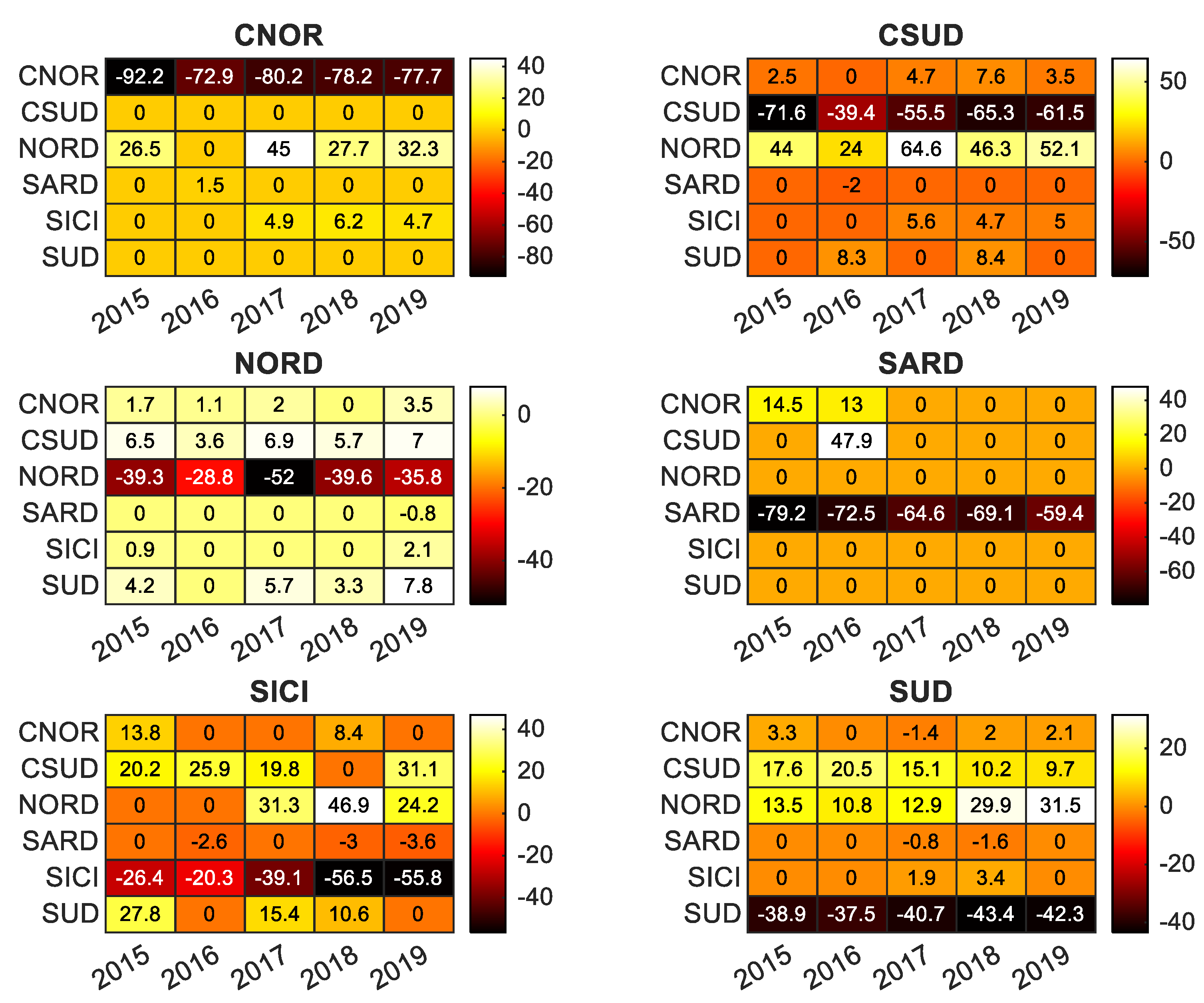
| CNOR | 2015 | 2016 | 2017 | 2018 | 2019 |
|---|---|---|---|---|---|
| ΔWind | −0.1081 *** | −0.0421 *** | −0.0494 *** | −0.0552 *** | −0.0523 *** |
| (0.0205) | (0.0135) | (0.018) | (0.0143) | (0.0103) | |
| ΔSolar | −0.0134 *** | −0.0104 *** | −0.0115 ** | −0.0141 *** | −0.0073 ** |
| (0.0048) | (0.0037) | (0.0052) | (0.0036) | (0.0033) | |
| ΔDemand | 0.0154 *** | 0.0124 *** | 0.0148 *** | 0.012 *** | 0.008 *** |
| (0.0022) | (0.0014) | (0.002) | (0.0012) | (0.0009) | |
| ΔNetIn | −0.0066 ** | −0.007 *** | −0.0068 *** | −0.0064 *** | 0.0013 |
| (0.0028) | (0.0019) | (0.0023) | (0.0016) | (0.0013) | |
| ΔNetInother zones | −0.0008 ** | −0.0007 *** | −0.0001 | −0.0002 | −0.0001 |
| (0.0003) | (0.0002) | (0.0003) | (0.0002) | (0.0003) | |
| ΔNGPrice | 0.3156 | 0.4129 ** | 1.1197 *** | 1.3786 *** | 0.6375 * |
| (0.6552) | (0.1924) | (0.2007) | (0.1415) | (0.3332) | |
| Dummies | Yes | Yes | Yes | Yes | Yes |
| Observations | 365 | 366 | 365 | 365 | 365 |
| Adjusted R2 | 0.40 | 0.38 | 0.44 | 0.51 | 0.43 |
| CSUD | 2015 | 2016 | 2017 | 2018 | 2019 |
|---|---|---|---|---|---|
| ΔWind | −0.0137 *** | −0.0081 *** | −0.0111 *** | −0.0076 *** | −0.0093 *** |
| (0.0013) | (0.0008) | (0.0012) | (0.001) | (0.0009) | |
| ΔSolar | −0.0092 *** | −0.0046 ** | −0.0107 *** | −0.0056 ** | −0.0042 * |
| (0.0031) | (0.0021) | (0.0033) | (0.0024) | (0.0023) | |
| ΔDemand | 0.01 *** | 0.0065 *** | 0.0074 *** | 0.0064 *** | 0.008 *** |
| (0.0009) | (0.0006) | (0.0009) | (0.0007) | (0.0007) | |
| ΔNetIn | −0.0044 *** | −0.0026 *** | 0.0004 | −0.0001 | −0.0001 |
| (0.001) | (0.0007) | (0.0008) | (0.0006) | (0.0007) | |
| ΔNetInother zones | −0.0002 | −0.0006 *** | −0.0003 | 0.0003 | 0 |
| (0.0003) | (0.0002) | (0.0003) | (0.0003) | (0.0003) | |
| ΔNGPrice | 0.2792 | 0.2395 | 1.3375 *** | 1.1819 *** | 0.6796 * |
| (0.6128) | (0.1759) | (0.1917) | (0.1411) | (0.346) | |
| Dummies | Yes | Yes | Yes | Yes | Yes |
| Observations | 365 | 366 | 365 | 365 | 365 |
| Adjusted R2 | 0.47 | 0.43 | 0.44 | 0.44 | 0.46 |
| NORD | 2015 | 2016 | 2017 | 2018 | 2019 |
|---|---|---|---|---|---|
| ΔWind | −0.0551 | −0.0047 | 0.0208 | −0.063 | −0.0235 |
| (0.0237) | (0.0446) | (0.0645) | (0.0617) | (0.0293) | |
| ΔSolar | −0.002 * | −0.0016 * | −0.0005 | −0.0034 *** | −0.0026 *** |
| (0.0011) | (0.001) | (0.0014) | (0.0011) | (0.0008) | |
| ΔDemand | 0.0023 *** | 0.0019 *** | 0.002 *** | 0.0016 *** | 0.0018 *** |
| (0.0001) | (0.0001) | (0.0002) | (0.0001) | (0.0001) | |
| ΔNetIn | −0.0025 *** | −0.0022 *** | −0.0018 *** | −0.0013 *** | −0.0015 *** |
| (0.0003) | (0.0002) | (0.0004) | (0.0003) | (0.0003) | |
| ΔNetInother zones | −0.0012 * | −0.0001 | 0.0011 | 0 | 0.0009 ** |
| (0.0006) | (0.0005) | (0.0007) | (0.0005) | (0.0004) | |
| ΔNGPrice | 0.2075 | 0.2375 | 1.2082 *** | 1.2649 *** | 0.4735 |
| (0.5492) | (0.1802) | (0.1944) | (0.1373) | (0.2933) | |
| Dummies | Yes | Yes | Yes | Yes | Yes |
| Observations | 365 | 366 | 365 | 365 | 365 |
| Adjusted R2 | 0.52 | 0.57 | 0.48 | 0.53 | 0.58 |
| SARD | 2015 | 2016 | 2017 | 2018 | 2019 |
|---|---|---|---|---|---|
| ΔWind | −0.0175 *** | −0.005 | −0.0153 *** | −0.0076 ** | −0.01 *** |
| (0.0039) | (0.0032) | (0.0043) | (0.0034) | (0.0028) | |
| ΔSolar | −0.0263 * | −0.0136 | −0.0538 *** | 0.0024 | −0.0699 *** |
| (0.0144) | (0.0118) | (0.0173) | (0.016) | (0.0167) | |
| ΔDemand | 0.068 *** | 0.0495 *** | 0.0364 *** | 0.0213 *** | 0.0128 *** |
| (0.0097) | (0.006) | (0.0078) | (0.0045) | (0.0033) | |
| ΔNetIn | −0.0087 ** | 0.0035 | −0.0041 | 0.0017 | 0.004 |
| (0.0038) | (0.0032) | (0.0046) | (0.0033) | (0.0028) | |
| ΔNetInother zones | 0.0007 ** | −0.0003 * | 0.001 *** | 0.001 *** | 0.0017 *** |
| (0.0003) | (0.0002) | (0.0003) | (0.0003) | (0.0003) | |
| ΔNGPrice | 0.439 | 0.2303 | 1.3876 *** | 1.3613 *** | 0.2344 |
| (0.7204) | (0.2018) | (0.224) | (0.1634) | (0.4352) | |
| Dummies | Yes | Yes | Yes | Yes | Yes |
| Observations | 365 | 366 | 365 | 365 | 365 |
| Adjusted R2 | 0.29 | 0.26 | 0.31 | 0.25 | 0.26 |
| SICI | 2015 | 2016 | 2017 | 2018 | 2019 |
|---|---|---|---|---|---|
| ΔWind | −0.0206 *** | −0.0196 *** | −0.0293 *** | −0.0357 *** | −0.0497 *** |
| (0.0018) | (0.0011) | (0.0016) | (0.002) | (0.0025) | |
| ΔSolar | −0.0242 *** | −0.0223 *** | −0.0163 * | −0.0239 *** | −0.036 *** |
| (0.0082) | (0.0057) | (0.009) | (0.0088) | (0.0105) | |
| ΔDemand | 0.0079 ** | 0.0162 *** | 0.034 *** | 0.0353 *** | 0.0567 *** |
| (0.0033) | (0.0021) | (0.0031) | (0.0038) | (0.0041) | |
| ΔNetIn | 0.0021 | −0.018 *** | −0.0228 *** | −0.0271 *** | −0.037 *** |
| (0.0051) | (0.0019) | (0.0024) | (0.003) | (0.0036) | |
| ΔNetInother zones | 0.0007 ** | −0.0003 | −0.0001 | 0.001 *** | 0.0002 |
| (0.0003) | (0.0002) | (0.0003) | (0.0004) | (0.0005) | |
| ΔNGPrice | 1.0011 | −0.4207 ** | 0.6942 *** | 0.9578 *** | −0.28 |
| (0.6794) | (0.19) | (0.2041) | (0.2161) | (0.6208) | |
| Dummies | Yes | Yes | Yes | Yes | Yes |
| Observations | 365 | 366 | 365 | 365 | 365 |
| Adjusted R2 | 0.41 | 0.42 | 0.57 | 0.56 | 0.63 |
| SUD | 2015 | 2016 | 2017 | 2018 | 2019 |
|---|---|---|---|---|---|
| ΔWind | −0.008 *** | −0.0056 *** | −0.0055 *** | −0.0057 *** | −0.0077 *** |
| (0.0006) | (0.0004) | (0.0005) | (0.0005) | (0.0005) | |
| ΔSolar | −0.0052 ** | −0.0029 ** | −0.003 | −0.0039 * | −0.002 * |
| (0.0024) | (0.0014) | (0.0025) | (0.002) | (0.0025) | |
| ΔDemand | 0.0122 *** | 0.0072 *** | 0.0074 *** | 0.0077 *** | 0.0126 *** |
| (0.0017) | (0.001) | (0.0015) | (0.0013) | (0.0015) | |
| ΔNetIn | −0.0007 | −0.0024 *** | −0.0005 | −0.0009 | −0.0031 *** |
| (0.0009) | (0.0006) | (0.0008) | (0.0007) | (0.0009) | |
| ΔNetInother zones | 0.0003 | −0.0003 * | 0.0005 * | 0.0013 *** | 0.0003 |
| (0.0003) | (0.0002) | (0.0003) | (0.0002) | (0.0003) | |
| ΔNGPrice | 0.5596 | −0.0713 | 1.2589 *** | 1.03 *** | 0.5423 |
| (0.6498) | (0.1631) | (0.1654) | (0.1367) | (0.4103) | |
| Dummies | Yes | Yes | Yes | Yes | Yes |
| Observations | 365 | 366 | 365 | 365 | 365 |
| Adjusted R2 | 0.44 | 0.41 | 0.48 | 0.44 | 0.47 |
References
- Union, E. Directive 2009/28/EC of the European Parliament and of the Council of 23 April 2009 on the promotion of the use of energy from renewable sources and amending and subsequently repealing Directives 2001/77/EC and 2003/30/EC. Off. J. Eur. Union 2009, 5, 2009. [Google Scholar]
- Contaldi, M.; Gracceva, F.; Tosato, G. Evaluation of green-certificates policies using the MARKAL-MACRO-Italy model. Energy Policy 2007, 35, 797–808. [Google Scholar] [CrossRef]
- Di Dio, V.; Favuzza, S.; La Cascia, D.; Massaro, F.; Zizzo, G. Critical assessment of support for the evolution of photovoltaics and feed-in tariff(s) in Italy. Sustain. Energy Technol. Assess. 2015, 9, 95–104. [Google Scholar] [CrossRef]
- GME-Gestore dei Mercati Energetici SpA. Available online: https://www.mercatoelettrico.org (accessed on 10 December 2020).
- Rintamäki, T.; Siddiqui, A.S.; Salo, A. Does renewable energy generation decrease the volatility of electricity prices? An analysis of Denmark and Germany. Energy Econ. 2017, 62, 270–282. [Google Scholar] [CrossRef] [Green Version]
- Deane, P.; Collins, S.; Gallachóir, B.Ó.; Eid, C.; Hartel, R.; Keles, D.; Fichtner, W. Quantifying the” merit-order” effect in European electricity markets. INSIGHT-E Rapid Response Energy Brief. 2015, 4. [Google Scholar] [CrossRef]
- Macedo, D.P.; Marques, A.C.; Damette, O. The Merit-Order Effect on the Swedish bidding zone with the highest electricity flow in the Elspot market. Energy Econ. 2021, 102, 105465. [Google Scholar] [CrossRef]
- Clò, S.; Cataldi, A.; Zoppoli, P. The merit-order effect in the Italian power market: The impact of solar and wind generation on national wholesale electricity prices. Energy Policy 2015, 77, 79–88. [Google Scholar] [CrossRef]
- Loumakis, S.; Giannini, E.; Maroulis, Z. Merit Order Effect Modeling: The Case of the Hellenic Electricity Market. Energies 2019, 12, 3869. [Google Scholar] [CrossRef] [Green Version]
- Gelabert, L.; Labandeira, X.; Linares, P. An ex-post analysis of the effect of renewables and cogeneration on Spanish electricity prices. Energy Econ. 2011, 33, S59–S65. [Google Scholar] [CrossRef]
- Woo, C.-K.; Horowitz, I.; Moore, J.; Pacheco, A. The impact of wind generation on the electricity spot-market price level and variance: The Texas experience. Energy Policy 2011, 39, 3939–3944. [Google Scholar] [CrossRef]
- Würzburg, K.; Labandeira, X.; Linares, P. Renewable generation and electricity prices: Taking stock and new evidence for Germany and Austria. Energy Econ. 2013, 40, S159–S171. [Google Scholar] [CrossRef] [Green Version]
- Macedo, D.P.; Marques, A.C.; Damette, O. The impact of the integration of renewable energy sources in the electricity price formation: Is the Merit-Order Effect occurring in Portugal? Util. Policy 2020, 66, 101080. [Google Scholar] [CrossRef]
- Cludius, J.; Hermann, H.; Matthes, F.C.; Graichen, V. The merit order effect of wind and photovoltaic electricity generation in Germany 2008–2016: Estimation and distributional implications. Energy Econ. 2014, 44, 302–313. [Google Scholar] [CrossRef]
- Benhmad, F.; Percebois, J. Photovoltaic and wind power feed-in impact on electricity prices: The case of Germany. Energy Policy 2018, 119, 317–326. [Google Scholar] [CrossRef]
- Nord Pool Sport. The Nordic Electricity Exchange and the Nordic Model for a Liberalized Electricity Market; Nord Pool Spot: Lysaker, Norway, 2009. [Google Scholar]
- Unger, E.A.; Ulfarsson, G.F.; Gardarsson, S.M.; Matthiasson, T. A long-term analysis studying the effect of changes in the Nordic electricity supply on Danish and Finnish electricity prices. Econ. Anal. Policy 2017, 56, 37–50. [Google Scholar] [CrossRef]
- O’Mahoney, A.; Denny, E. The merit order effect of wind generation on the Irish electricity market. In Proceedings of the 30th USAEE/IAEEE North American Conference, Washington, DC, USA, 9–12 October 2011. [Google Scholar]
- Sirin, S.M.; Yilmaz, B.N. Variable renewable energy technologies in the Turkish electricity market: Quantile regression analysis of the merit-order effect. Energy Policy 2020, 144, 111660. [Google Scholar] [CrossRef]
- Quint, D.; Dahlke, S. The impact of wind generation on wholesale electricity market prices in the midcontinent independent system operator energy market: An empirical investigation. Energy 2019, 169, 456–466. [Google Scholar] [CrossRef]
- Amor, M.B.; de Villemeur, E.B.; Pellat, M.; Pineau, P.-O. Influence of wind power on hourly electricity prices and GHG (greenhouse gas) emissions: Evidence that congestion matters from Ontario zonal data. Energy 2014, 66, 458–469. [Google Scholar] [CrossRef]
- Csereklyei, Z.; Qu, S.; Ancev, T. The effect of wind and solar power generation on wholesale electricity prices in Australia. Energy Policy 2019, 131, 358–369. [Google Scholar] [CrossRef]
- Gianfreda, A.; Parisio, L.; Pelagatti, M. The impact of RES in the Italian day–ahead and balancing markets. Energy J. 2016, 37, 161–184. [Google Scholar] [CrossRef] [Green Version]
- Imani, M.H.; Bompard, E.; Colella, P.; Huang, T. Predictive methods of electricity price: An application to the Italian electricity market. In Proceedings of the 2020 IEEE International Conference on Environment and Electrical Engineering and 2020 IEEE Industrial and Commercial Power Systems Europe (EEEIC/I&CPS Europe), Madrid, Spain, 9–12 June 2020; IEEE: Piscataway, NJ, USA, 2020; pp. 1–6. [Google Scholar]
- ENTSO-E. Available online: https://www.entsoe.eu/ (accessed on 10 December 2020).
- Figueiredo, N.C.; da Silva, P.P. The “Merit-order effect” of wind and solar power: Volatility and determinants. Renew. Sustain. Energy Rev. 2019, 102, 54–62. [Google Scholar] [CrossRef]
- Pantula, S.G.; Gonzalez-Farias, G.; Fuller, W.A. A comparison of unit-root test criteria. J. Bus. Econ. Stat. 1994, 12, 449–459. [Google Scholar]
- Breusch, T.S.; Pagan, A.R. A simple test for heteroscedasticity and random coefficient variation. Econom. J. Econom. Soc. 1979, 47, 1287–1294. [Google Scholar] [CrossRef]
- Newey, W.K.; West, K.D. A Simple, Positive Semi-Definite, Heteroskedasticity and Autocorrelationconsistent Covariance Matrix; National Bureau of Economic Research: Cambridge, MA, USA, 1986. [Google Scholar]
- Zarnikau, J.; Tsai, C.H.; Woo, C.K. Determinants of the wholesale prices of energy and ancillary services in the US Midcontinent electricity market. Energy 2020, 195, 117051. [Google Scholar] [CrossRef]
- MacKinnon, J.G. Numerical distribution functions for unit root and cointegration tests. J. Appl. Econom. 1996, 11, 601–618. [Google Scholar] [CrossRef] [Green Version]


| Zone | Input Variables | 2015 | 2016 | 2017 | 2018 | 2019 |
|---|---|---|---|---|---|---|
| CNOR | ΔWind | −0.5394 *** | −0.8065 *** | −0.8757 *** | −0.7107 *** | −0.652 *** |
| (0.1904) | (0.1443) | (0.1361) | (0.1337) | (0.1368) | ||
| ΔSolar | −0.922 *** | −0.7291 *** | −0.8023 *** | −0.7821 *** | −0.7772 *** | |
| (0.0215) | (0.0173) | (0.0211) | (0.0189) | (0.0237) | ||
| ΔDemand | 0.7426 *** | 0.7553 *** | 0.7527 *** | 0.722 *** | 0.6984 *** | |
| (0.0095) | (0.0091) | (0.0119) | (0.0103) | (0.0114) | ||
| ΔWindother zones | 0.0322 *** | 0.0376 *** | 0.0324 *** | 0.0339 *** | 0.0538 *** | |
| (0.0049) | (0.005) | (0.0042) | (0.0038) | (0.0044) | ||
| ΔSolarother zones | 0.0297 *** | 0.0057 ** | 0.0112 *** | 0.0172 *** | 0.0314 *** | |
| (0.0031) | (0.0025) | (0.003) | (0.0027) | (0.0034) | ||
| ΔDemandother zones | −0.0083 *** | −0.01 *** | −0.01 *** | −0.0081 *** | −0.014 *** | |
| (0.0013) | (0.0012) | (0.0015) | (0.0014) | (0.0015) | ||
| Dummies | Yes | Yes | Yes | Yes | Yes | |
| Observations | 8760 | 8784 | 8760 | 8760 | 8760 | |
| Adjusted R2 | 0.83 | 0.80 | 0.82 | 0.82 | 0.72 | |
| SICI | ΔWind | −0.4463 *** | −0.5383 *** | −0.6949 *** | −0.7151 *** | −0.74 *** |
| (0.0146) | (0.0183) | (0.0199) | (0.0166) | (0.0182) | ||
| ΔSolar | −0.2639 *** | −0.2032 *** | −0.3915 *** | −0.5646 *** | −0.5576 *** | |
| (0.0195) | (0.0262) | (0.0303) | (0.0252) | (0.029) | ||
| ΔDemand | 0.0941 *** | 0.111 *** | 0.2949 *** | 0.377 *** | 0.3923 *** | |
| (0.0103) | (0.013) | (0.0163) | (0.0145) | (0.0167) | ||
| ΔWindother zones | 0.0268 *** | 0.0364 *** | 0.049 *** | 0.0585 *** | 0.0313 *** | |
| (0.0045) | (0.006) | (0.006) | (0.0054) | (0.0051) | ||
| ΔSolarother zones | 0.0083 *** | 0.0004 | 0.0126 *** | 0.0167 *** | 0.0169 *** | |
| (0.0018) | (0.0024) | (0.0027) | (0.0023) | (0.0026) | ||
| ΔDemandother zones | −0.0082 *** | −0.0052 *** | −0.0118 *** | −0.0109 *** | −0.0096 *** | |
| (0.0007) | (0.0009) | (0.0011) | (0.001) | (0.0011) | ||
| Dummies | Yes | Yes | Yes | Yes | Yes | |
| Observations | 8760 | 8784 | 8760 | 8760 | 8760 | |
| Adjusted R2 | 0.14 | 0.13 | 0.19 | 0.30 | 0.28 |
| Zone | Input Variables | 2015 | 2016 | 2017 | 2018 | 2019 |
|---|---|---|---|---|---|---|
| CNOR | ΔWind | −0.1081 *** | −0.0421 *** | −0.0494 *** | −0.0552 *** | −0.0523 *** |
| (0.0205) | (0.0135) | (0.018) | (0.0143) | (0.0103) | ||
| ΔSolar | −0.0134 *** | −0.0104 *** | −0.0115 ** | −0.0141 *** | −0.0073 ** | |
| (0.0048) | (0.0037) | (0.0052) | (0.0036) | (0.0033) | ||
| ΔDemand | 0.0154 *** | 0.0124 *** | 0.0148 *** | 0.012 *** | 0.008 *** | |
| (0.0022) | (0.0014) | (0.002) | (0.0012) | (0.0009) | ||
| ΔNetIn | −0.0066 ** | −0.007 *** | −0.0068 *** | −0.0064 *** | 0.0013 | |
| (0.0028) | (0.0019) | (0.0023) | (0.0016) | (0.0013) | ||
| ΔNetInother | −0.0008 ** | −0.0007 *** | −0.0001 | −0.0002 | −0.0001 | |
| (0.0003) | (0.0002) | (0.0003) | (0.0002) | (0.0003) | ||
| ΔNGPrice | 0.3156 | 0.4129 ** | 1.1197 *** | 1.3786 *** | 0.6375 * | |
| (0.6552) | (0.1924) | (0.2007) | (0.1415) | (0.3332) | ||
| Dummies | Yes | Yes | Yes | Yes | Yes | |
| Observations | 365 | 366 | 365 | 365 | 365 | |
| Adjusted R2 | 0.40 | 0.38 | 0.44 | 0.51 | 0.43 | |
| SICI | ΔWind | −0.0206 *** | −0.0196 *** | −0.0293 *** | −0.0357 *** | −0.0497 *** |
| (0.0018) | (0.0011) | (0.0016) | (0.002) | (0.0025) | ||
| ΔSolar | −0.0242 *** | −0.0223 *** | −0.0163 * | −0.0239 *** | −0.036 *** | |
| (0.0082) | (0.0057) | (0.009) | (0.0088) | (0.0105) | ||
| ΔDemand | 0.0079 ** | 0.0162 *** | 0.034 *** | 0.0353 *** | 0.0567 *** | |
| (0.0033) | (0.0021) | (0.0031) | (0.0038) | (0.0041) | ||
| ΔNetIn | 0.0021 | −0.018 *** | −0.0228 *** | −0.0271 *** | −0.037 *** | |
| (0.0051) | (0.0019) | (0.0024) | (0.003) | (0.0036) | ||
| ΔNetInother | 0.0007 ** | −0.0003 | −0.0001 | 0.001 *** | 0.0002 | |
| (0.0003) | (0.0002) | (0.0003) | (0.0004) | (0.0005) | ||
| ΔNGPrice | 1.0011 | −0.4207 ** | 0.6942 *** | 0.9578 *** | −0.28 | |
| (0.6794) | (0.19) | (0.2041) | (0.2161) | (0.6208) | ||
| Dummies | Yes | Yes | Yes | Yes | Yes | |
| Observations | 365 | 366 | 365 | 365 | 365 | |
| Adjusted R2 | 0.41 | 0.42 | 0.57 | 0.56 | 0.63 |
| Impact on Zonal Price | ||
|---|---|---|
| Zone | Wind | Solar |
| CNOR | −10% | −1.4% |
| CSUD | −1.77% | −0.8% |
| NORD | 0% | −0.5% |
| SARD | −1.93% | −13.5% |
| SICI | −7.92% | −5.7% |
| SUD | −1.52% | −0.39% |
Publisher’s Note: MDPI stays neutral with regard to jurisdictional claims in published maps and institutional affiliations. |
© 2021 by the authors. Licensee MDPI, Basel, Switzerland. This article is an open access article distributed under the terms and conditions of the Creative Commons Attribution (CC BY) license (https://creativecommons.org/licenses/by/4.0/).
Share and Cite
Hosseini Imani, M.; Bompard, E.; Colella, P.; Huang, T. Impact of Wind and Solar Generation on the Italian Zonal Electricity Price. Energies 2021, 14, 5858. https://doi.org/10.3390/en14185858
Hosseini Imani M, Bompard E, Colella P, Huang T. Impact of Wind and Solar Generation on the Italian Zonal Electricity Price. Energies. 2021; 14(18):5858. https://doi.org/10.3390/en14185858
Chicago/Turabian StyleHosseini Imani, Mahmood, Ettore Bompard, Pietro Colella, and Tao Huang. 2021. "Impact of Wind and Solar Generation on the Italian Zonal Electricity Price" Energies 14, no. 18: 5858. https://doi.org/10.3390/en14185858