Article

Recognizing VSC DC Cable Fault Types Using Bayesian Functional Data Depth

by
Jerzy Baranowski
*,
Katarzyna Grobler-Dębska
and
Edyta Kucharska
Department of Automatic Control and Robotics, AGH University of Science and Technology, Al. Mickiewicza 30, 30-059 Kraków, Poland
*
Author to whom correspondence should be addressed.
Energies 2021, 14(18), 5893; https://doi.org/10.3390/en14185893
Submission received: 16 August 2021 / Revised: 12 September 2021 / Accepted: 15 September 2021 / Published: 17 September 2021
(This article belongs to the Collection Women's Research in Smart Energy Systems)

Abstract

:
Diagnostics of power and energy systems is obviously an important matter. In this paper we present a contribution of using new methodology for the purpose of signal type recognition (for example, faulty/healthy or different types of faults). Our approach uses Bayesian functional data analysis with data depths distributions to detect differing signals. We present our approach for discrimination of pole-to-pole and pole-to-ground short circuits in VSC DC cables. We provide a detailed case study with Monte Carlo analysis. Our results show potential for applications in diagnostics under uncertainty.

1. Introduction

Effective and reliable monitoring and diagnostics of energy installations is of utmost importance, as they are an important part of the world’s economy. Algorithms for fault detection and isolation allow extension of system lifetime, reduction in operation interruption and can lead to significant savings. The main difficulty in their development is that power installations have a high level of complexity, are usually nonlinear and are influenced by stochastic disturbances and parameter variations. Therefore, approaches based on first principles models are difficult or even impossible to use on a wider scale. That is why methods based on statistical models or machine learning are those most researched.
Typically, machine learning, data-driven models are providing complicated ‘black-box’ models, which are not transparent and hard to interpret. This means flaws are less prevalent in statistical approaches which is a cause of their dominance of statistical approaches in the field. Both of those groups, however, suffer from the typical situation that the real data for system faults is extremely rare, and even if present it is often incomplete. That is why it is crucial to develop methods that can handle issues of non-representative or missing data. Bayesian methods are an emerging set of tools for solving many kinds of diagnostic problems [1,2,3].
Time series diagnostics are usually based on extracting features and with that reduction of dimensionality as signals are represented as vectors of numbers. Unfortunately the usual approach to feature extraction is to obtain certain typical statistical measures (such as mean, standard deviation, kurtosis, median, peak-to-peak) in both time and frequency domain and hope that they will contain enough information about the signal [4,5]. This negatively influences reliability and efficiency of diagnostic models as it is very hard to verify. In the case of transient diagnostics authors (e.g., [6]), they mostly use autoregressive moving average models (or their variants) which is a significant limitation both because of linearity and non-locality (it is difficult to capture localized behavior). Many cable fault location studies are based on simulation models and methods and use simulation tools.
Functional data analysis (FDA) is a group of methods for analysis of data in the form of functions, with a special focus on time series data. The main idea is to create a model of the signal using certain function basis and coefficients of that basis representation can be considered as reduced dimensionality. FDA is a matured field in the area of statistics, with focus on bases in functional spaces such as polynomials, wavelets and others. Maturity of the field can be observed by recent review papers [7] or special issues [8] in prestigious journals covering the field of statistics. We join FDA with Bayesian approach in order to obtain probability distributions of basis coefficients, get generative models and model uncertainty.
In the case of cable fault monitoring, popular approaches are based on first principle model fitting. In the next section we provide a comprehensive overview of such methods. An important aspect shared by all those methods is that they are not focused on uncertainty. They are often considering point estimates or least squares fits. In this paper we want to provide a certain proof of concept for using statistical methods for fault detection and distinguishing types of faults. For this purpose we focus on a real problem of distinguishing between pole-to-ground and pole-to-pole short circuits. Pole-to-pole and pole-to-ground short circuits are the typical DC cable faults. These generally result in fast discharge of the DC-link capacitor through the DC circuit, leading to transient overcurrent, which can damage system components. In addition to fault type and DC system parameters (namely, capacitance C of the DC-link capacitor and cable distributed parameters Rx, Lx), transient response also depends on fault distance x and fault resistance Rf. VSC DC systems are helpless against these DC faults because IGBTs are blocked for self-protection during the fault, leaving freewheel diodes subject to overcurrent [9].
We propose a general algorithm for comparing signals with reference that takes uncertainty under account and uses functional data analysis to provide dimensionality reduction. Uncertainty modeling is obviously important to avoid ill-informed decisions.
Our main contributions are:
  • Construction of Bayesian spline model capturing measurement and parameter uncertainty,
  • An algorithm for using Bayesian models to obtain data depth distributions allowing analysis of signal similarity,
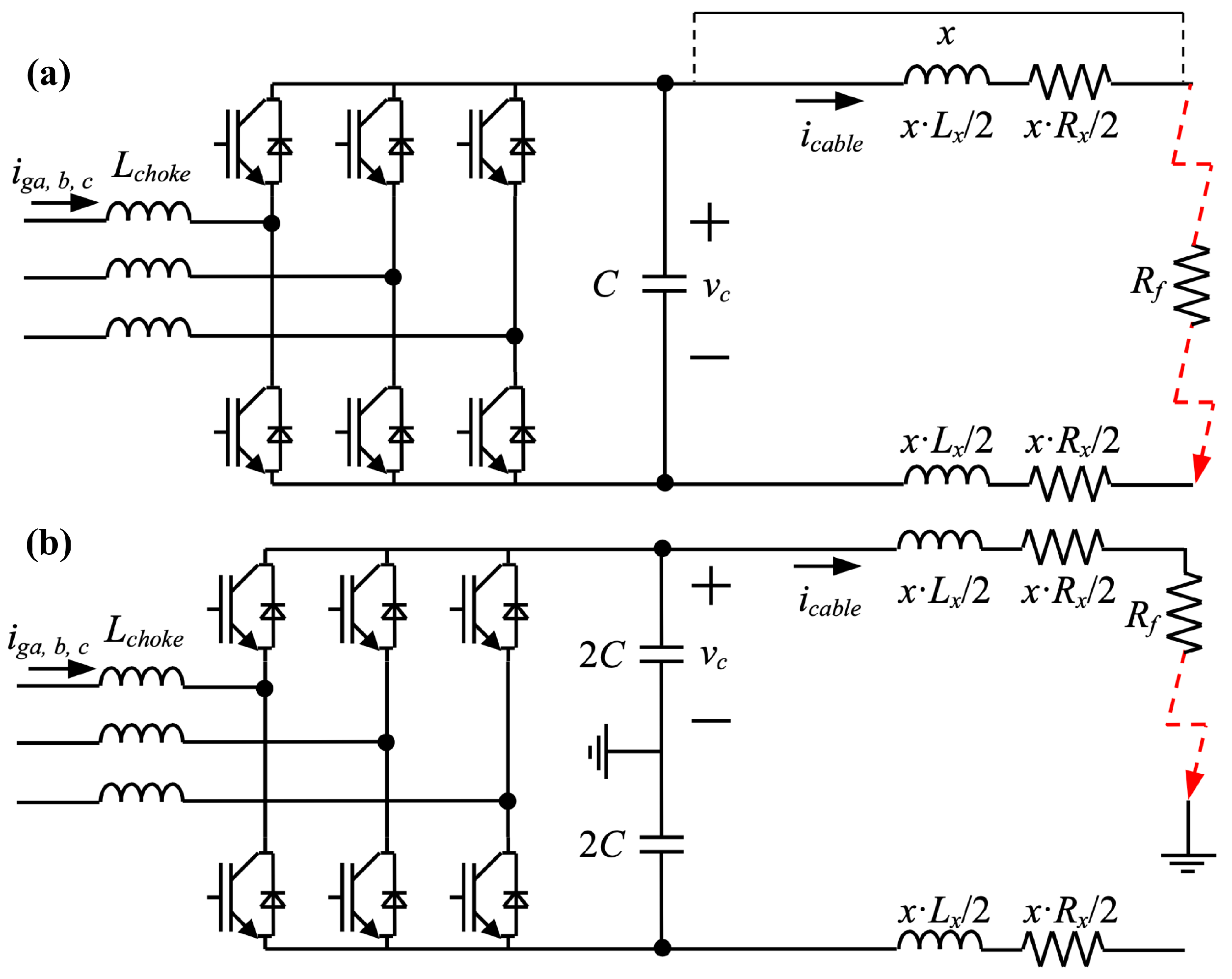
  • An extended case study using simulated voltage source converter (VSC) direct current DC cable fault data focusing on pole-to-pole and pole-to-ground short circuits.
The rest of the paper is organized as follows. First we present a review of cable fault modeling techniques. Then we present methodologies behind data depth and spline modeling using Bayesian hierarchical linear model. Then we describe our computational system and thoroughly analyze current and voltage signals as an indicator, allowing distinguishing between fault types. We finish the paper with the discussion and conclusions section.

2. Review of Cable Fault Modeling Research

Pollution, physical damage, aging and environmental impact may generate the fault of the cable and cause a variety of serious consequences. It is crucial to detect and locate the cable fault fast and accurately, in particular in case of aircraft cable. Because of this, cable system behavior under fault conditions needs to be studied to enable rapid interruption and isolation of damage. Therefore, many research papers deal with this problem.
In literature, papers present methods and algorithms detecting and locating faults based on simulations and also propose a theoretical analysis of different cable faults.
Many papers investigate VSC DC system by performing various types of computer simulations. Paper [9] deals with two-level VSC DC system response to DC cable faults and analytical expressions for characterizing DC fault overcurrent and voltages and identifying main DC fault characteristics. Yang et al. [10] investigate DC cable transient modeling issues for VSC based high voltage direct current (HVDC) transmission systems. Loume [11] focuses on the influence of cable modeling and grounding on DC fault current behavior in a HVDC point-to-point cable system. In [12] authors propose a transient simplified model with high-frequency components of the fault DC network reserved.
A different important problem is designing extensive networks so that cable failures do not cause further undesirable consequences.
Zhang et al. [13] present a sub-sea DC collection grid with robust control and protection scheme with the DC/DC converter. Network section interconnections are decoupled in the event of DC faults. Jovic et al. [14] consider building large DC grids as an interconnection of regional radial DC systems, which enables very simple and robust DC system protection. An interesting approach is also the one of Bapijaru et al. [15], who present cable models. Their purpose is the analysis of the faults’ nature using signatures of measurements in offshore Multi-Modular Converter High Voltage DC (MMC-HVDC) systems.
Cable location studies rely mostly on simulation models, methods and tools. In particular, this concerns the underground power cables [16]. PSCAD™EMTP [17,18] and PROTEUS version 8.1 [19] are the examples of the simulation tools used in cable diagnosis. Gjabhiye et al. [20] review various fault locating methods and highly computational methods for underground cables and provide design of fault location and remote indicators.
In particular, it covers various types of methods (A-Frame Method, A-Frame Method, Time Domain Reflectometry (TDR) and Bridge Method) and highlights the adverse effects of some of them and the selection of methods to the type of fault. The authors in [21] propose new method for online monitoring underground cable monitoring. The simulation tool PSCAD/EMTDC is popular for fault model verification. In paper [22] authors present model for both type pole-to-ground and the pole-to-pole faults detection for cables used in photovoltaics (PV). In paper [23] authors present simulation model of sheath earth current generation and the relationship between sheath earth current and load current. This model simulates various faults of sheath grounding system.
Diagnostic systems for high voltage cables based on sheath current are also an important issue. The sheath current is measured to locate a segment of transversely connected fault, which leads to reduced maintenance time. In the paper [24] authors present an equivalent circuit model of sheath current in a cross-connected cable system according to the single-wire laying type. The model considers the operating mode, cable parameters and line length. This paper [25] presents a model for cable over sheath damage at alternating current (AC) voltage. Authors propose representation of the characteristics as a combination of linear resistance and capacitance. The model is implemented in Alternative Transient Program (ATP) by using the true nonlinear resistance model and transient analysis of control systems (TACS-controlled) switch.
The monitoring and diagnostic systems are designed also for Shielded Twisted Pair cables so that there is no interference between the twisted pair cables. The paper [26] discusses computer models of electrical wires in Shielded Twisted Pair cables and test procedures based on an Enhanced Time Domain Reflectometry technique. The diagnostic models for the coaxial cable are under consideration in papers [27,28]. In [27] faults of the cables are modeled as radiating apertures using the Bethe theory. In the paper [28], Shi et al. present the lossy transmission line model using time domain reflectometry and impedance spectroscopy for the extraction of parameters.
Few papers use predictive methods and data analysis to predict the occurrence of cable fault and the location of it. Such methods include Backpropagation (BP) neural network and Levenberg–Marquardt data-optimized method [29], recursive regression analysis and the amnesic factor regression analysis [30] and the method of data fusion based on Bayes estimate [31]. Successful applications of these methods include locating of cable faults and parameter estimation (e.g., resistance, inductance, conductance and capacitance).
In conclusion, our approach is a good supplement to existing methodology, as it is at least partially data driven, uncertainty focused and relatively simple. It fills certain gaps and has a potential for greater development.

3. Materials and Methods

In this section we introduce the main concepts on which our work is built. Firstly, we introduce the data depth function, which is certain measure of similarity of a multivariate datapoint to certain probability distribution. Then we present the idea for construction of Bayesian functional data models with splines. Finally, we give the algorithm for comparing signals to reference.

3.1. Data Depth

Data depth, as proposed by Tukey in 1975 [32], was considered a multivariate generalization of median, so a function that allows certain ordering of datapoints with respect to distribution. Data depth has multiple uses. Idris considered it for multivariate control charts for easier control of multidimensional processes [33]. Chenouri used it for improving the quality of nonparametric tests [34]. Nagy and Ferraty [35] use functional data analysis to represent discontinuous data. It was also used to analyze functional data [36,37]. By analyzing function curves, it is much easier to detect distant data. In addition, finding anomalies is easier by using the data depth derived from the functional mean.
We define the data depth as the distance of the measurements from the center of the point x R d regarding a distribution function F. The outermost observations have lower values than the near-center data. They are determined by the depth function. This way, you can identify which data is anomalous throughout the process. First, let us start with the definition of the depth function.
Let the mapping D ( · ; · ) : R d × F R be bounded, non-negative and meet the assumptions:’
  • D ( A x + b ; F A X + b ) = D ( x ; F X ) holds for any random vector X in R d , any d × d nonsingular matrix A and any d-vector b;
  • D ( θ ; F ) = s u p x R d D ( x ; F ) holds for any F F having center θ ;
  • for any F F having deepest point θ , D ( x ; F ) D ( θ + α ( x θ ) ; F ) holds for α [ 0 , 1 ] ;
  • D ( x ; F ) 0 as x , for each F F .
Then D ( · ; F ) is called a statistical depth function [38].
There are multiple definitions fulfilling depth function conditions. Tukey proposed the half space depth, known also as Tukey depth or location depth. In the following years, researchers proposed new types like Euclidean depth, L p depth, Mahalanobis depth, projection depth, Oja depth and many others [39,40]. Those definitions have various properties, but for practical use, most important are computational complexity and scaling properties. Tukey’s depth has complexity of O ( 2 n ) , with n being number of dimensions, which makes it practically useless for high dimensional problems. Oja’s depth uses n-dimensional volumes of simplexes and has a complexity of O ( n 4 ) . Unfortunately, because of the curse of dimensionality, simplex volume in high-dimensional space can be infinitesimally small and get lost in rounding errors. Projection depth could be attractive but requires solution of n dimensional convex programming problem, which is hard to bound in the number of multiplications. Other mentioned depths have fewer problems, with best and most efficient results we obtained for Mahalanobis depth, which we define below.

Mahalanobis Depth

Mahalanobis proposed a method of determining the distance between two points x and y in R d in the following form
d M 2 ( x , y ) = ( x y ) M ( x y )
where M is positive definite d × d matrix.
Based on the Mahalanobis distance, the depth function can be defined as
M H D ( x ; F ) = 1 + d Σ ( F ) 2 ( x , μ ( F ) ) 1
where Σ ( F ) is covariance matrix of F and μ ( F ) is the mean.

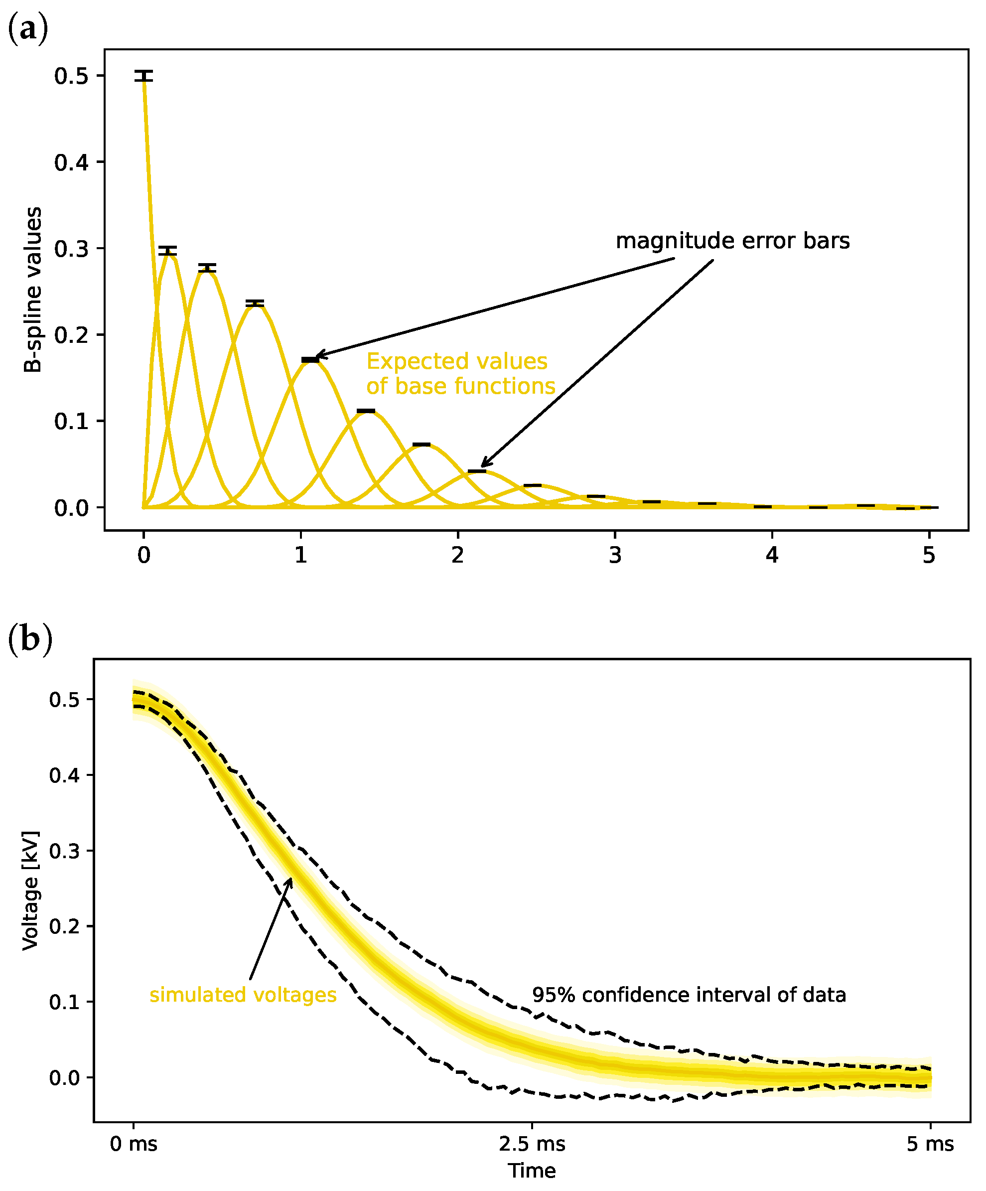
3.2. Bayesian Functional Spline Models

In this section we will not cover main principles of Bayesian statistics, for more details we refer the reader to Gelman’s book [41]. In the main principle we will be creating a joint probability distribution model for data and parameters.
We consider that our data generating process is given by
y n N ( μ n , σ ) μ n = m = 1 M θ m ϕ m ( t n )
where y n are our sampled measurements, n = 1 , , N , which with uncertainty of normal distribution given by σ . Functions ϕ m ( t ) are B-splines on the assigned M knot grid. μ n are transformed parameters of the model, as it corresponds to the mean of fitted distribution for individual measurements. It could be avoided, as actual model parameters are coefficients of B-splines combination θ m , but it improves formula clarity. θ m are all distributed with respect to normal distribution
θ m N ( μ 0 , σ 0 )
Parameters μ 0 , σ 0 are not known and are inferred from data, making the proposed model a hierarchical one. Relations of the entire model are presented using Bayesian network plate notation in Figure 1.
We can join the likelihood (3) and the hyper-prior (4) to construct a full model, assigning priors for all the parameters:
y n N ( μ n , σ ) n = 1 , , N μ n = m = 1 M θ m ϕ m ( t n ) θ m N ( μ 0 , σ 0 ) m = 1 , , M σ Exponential ( 1 ) μ 0 , σ 0 Uniform
Hyper-parameters were given uniform priors, as we have no justification for others, but as well they could be just disperse normals. σ was given an exponential prior, as it has heavier tail than half-normal allowing extra flexibility. The proposed model allows sampling of parameters from posterior and sampling from posterior predictive distribution. Posterior predictive distribution is a useful tool for generating predicted data from inferred parameters. For the rest of the paper we will refer to (5) as ‘model’.
Parameters θ m of the model are dimensionality reduction representation of the time series. Their number M is naturally smaller than number of samples N. However, those coefficients with basis functions allow for the representation of the signal up to the confidence interval.

3.3. Algorithm for Fault Determination and Detection

Here we will propose a data-driven general Bayesian algorithm using data depths and Bayesian functional models to capture uncertainty and compare signals to reference.
Main use of data-depth is the possibility of using it with data, as a statistic similar to the median. Its usefulness reduces if data is not available in large quantities. However, having a model of data generating process using posterior predictive distribution one can generate as many datapoints are needed efficiently estimating data depth. This is the base of our algorithm.
Algorithm consists of the following steps:
  • Create reference. Having a set of reference signals (for example, healthy behavior). Fit the model with them and obtain the set of samples of ( θ m ) M sequences.
  • Compute Mahalanobis depth distribution. Using the obtained samples, compute mean and covariance matrices and determine depth of each of the samples. This will be our reference depth distribution. It can be summarized by a histogram if needed.
  • Create model of the candidate. Using the same model, fit it with the candidate signal and obtain the set of samples of ( θ m ) M sequences.
  • Compute the depth distribution of candidate with respect to reference. Using mean and covariance of the reference set compute the Mahalanobis depth of all the samples of the candidate. This gives a marginal probability distribution of depth of candidate with respect to reference.
  • Analyze the overlap/distance. The marginal distribution of the depth allows us to verify if signal is ‘shallow’ with respect to the reference set or close to it. If there is an overlap we can state that the similarity is strong. If there is a large gap, we can say that the signal is an ‘outlier’ with respect to reference.
The main strength of the proposed approach is that it allows to compensate for a small amount of data and its quality. Because the model of the candidate is available we can capture uncertainty coming from the disturbances and protect ourselves from accidentally stating that the signal is similar.

4. Results

In this section we present results of our case study applying our algorithm to determining in the VSC DC cable the type of fault between pole-to-pole and pole-to-ground short circuits. First we provide a brief description of our data. Then we describe the computational system used. Finally, we go in depth in to analysis of current and voltage signals for their diagnostic use.

4.1. Considered Data

For our data we have considered results from simulation models given by Mesas et al. [9] for configurations presented in Figure 2. Proposed models represent the initial 5 ms period after the fault occurrence. For those signals we have simulated with randomized parameters 100 voltage-current pairs for both pole-to-pole and pole-to-ground faults. We have taken parameters normally distributed with means equals to parameters provided by Mesas et al. and standard deviations corresponding to 10% of those values. Simulated signals are presented in Figure 3.

4.2. Computational Setup

For Bayesian computation, we have used Hamiltonian Monte Carlo (HMC, also known as hybrid Monte Carlo) algorithm. Currently, most advanced HMC software is Stan [42]. HMC algorithm is a type of Markov Chain Monte Carlo (MCMC) method. MCMC generates a Markov chain of samples. It generates them in a way that makes their limiting distribution converge to the desired probability distribution. MCMC methods are especially useful for Bayesian computation, as sampling from the posterior distribution is difficult. Using generated samples, we can estimate expected values of desired functions of random variables. Because of that, we can answer practically all relevant statistical questions.
HMC is a variant of the Metropolis–Hastings algorithm. Traditionally Metropolis–Hastings algorithm uses Gaussian random walk proposal distribution. Algorithm accepts or rejects samples from the random walk depending on computed acceptance probability. In HMC, we generate proposals of random variables (system states) through a Hamiltonian dynamics evolution. This evolution is simulated using a time-reversible and volume-preserving numerical integrator (a symplectic integrator). HMC algorithm reduces the correlation between successive sampled states by proposing moves to distant states. Those states maintain a high probability of acceptance. This happens because symplectic integrators conserve energy of the simulated Hamiltonian dynamic. The reduced correlation in HMC means we need fewer Markov chain samples to get a desired level of Monte Carlo error when computing expectations.
Simulation of Hamiltonian dynamics might numerically destabilize for probability distributions with complicated geometry. This is an advantage of the method, because such complications usually mean problems in identifiability of parameters. Destabilization (known in the statistical field as “divergence’’) is a useful diagnostic that can suggest re-parametrization or other numerical adaptation of algorithm.
All the codes used for computation in this paper are available in the repository listed at the “data availability’’ section.
For model computation we have decided to use limited sample of 10 signals in order to increase the uncertainty and reduce averaging. We have assigned a spline base of 15 third order polynomials which are presented in the Figure 4. As a reference we have selected pole-to-pole faults data and we were comparing them with pole-to-ground. This had no influence as results in the other way are very similar.

4.3. Analysis of Current Measurements

First we have started with analyzing current signals. The reference set was created with 10 selected signals. Results of the fit are presented in Figure 5. Here we have visualization of uncertainty of parameters of combination in the form of error bars Figure 5a and posterior predictive distribution compared to quantiles of data, Figure 5b. As we can see there is an underestimation of uncertainty in the middle of the signal.
Some statistics of inference are given in the Table 1. Hyper-prior parameters of the current spline model are efficiently estimated. They get very thin distributions centered in the neighbourhood of zero. Standard error of the current measurement is estimated at 0.05 kA which is consistent with simulations. Probabilistic computation is efficient, as Monte Carlo standard error (MCSE) is vanishingly small. Effective sample size of both bulk of distribution and its tails is on the level of 42% (total number of samples is 4000), which is a reasonable result. Figure 6 shows the distributions of the remaining parameters.
In Figure 7 we present the application of the algorithm to two samples, one of pole-to-pole and one of pole-to-ground faults. (a) Bayesian model has efficiently captured the shape of measurements. (b) Distribution of data depth shows good discrimination of pole-to-ground from the reference depth; however, isolated pole-to-pole fault is also much more shallow. It suggests that current is a poor diagnostic indicator in this case. It is further highlighted in Table 2. When analyzing current signal in the context of reference depth of pole-to-pole fault (with mean of 6.23 × 10 2 and spreading from 1.993 × 10 2 to 2.14 × 10 1 ) we can see that it is not the best indicator. While pole-to-ground scenarios are being clearly discriminated as ‘shallow’ with depths at the level of 10 5 , the pole-to-pole current signals are also separated from the reference, not getting depths greater than 10 3 .

5. Analysis of Voltage Measurements

We have then continued our analysis with the voltage signal. As previously, we have used 10 signals for reference using the voltages corresponding to previously included currents. Similarly we have fitted the model which is illustrated in Figure 8. The fit is slightly better at the end of the signal without overestimation.
Inference statistics are given in Table 3. Hyper-prior parameters of the voltage spline model are also efficiently estimated but with more difficulty. They get very thin distributions centered in the neighborhood of zero; however, all of them are positive. Standard error of the voltage measurement is estimated at 0.02 kV which is consistent with simulations. Probabilistic computation is efficient, as Monte Carlo standard error (MCSE) is vanishingly small. Effective sample size of both bulk of distribution and its tails is on the level between 15% and 25% (total number of samples is 4000), which is a reasonable result.
Potential scale reduction factor R ^ is reasonably close to 1, indicating good mixing of Markov chains. Kernel density estimators (Figure 9) of (a) hyper-parameters μ 0 , σ 0 and (b) standard error of voltage measurement also show reasonable sampling behavior. All the distributions are reasonably normal-like.
Figure 10 presents the application of the algorithm to two voltage samples, one of pole-to-pole and one of pole-to-ground faults. (a) Bayesian model has efficiently captured the shape of measurements. (b) Distribution of data depth shows good discrimination of pole-to-ground from the reference depth. Isolated pole-to-pole fault is also shallower than reference but reasonably close. It suggests that voltage is a much better diagnostic indicator in this case. It is also supported by the analysis in Table 4.

6. Discussion and Conclusions

The results presented in this paper are obviously in an early stage. Certainly there is a potential for diagnostic use of functional Bayesian models with data depth as a statistic. This application can find a place in energy systems, for example, in cable diagnostics. Certain aspects still require consideration. Perhaps a more varied reference set would provide better performance. This will certainly be investigated. We have also arbitrarily chosen the spline basis. Proper selection of order could be for example made using leave one out cross validation or Watanabe–Akaike Information Criterion. Those are aspects that we will continue to investigate. Finally, we want to investigate the method for joining both signals for diagnostics (a functional data fusion); this is also an open challenge.

Author Contributions

Conceptualization, J.B.; methodology, J.B.; software, J.B.; validation, J.B., E.K. and K.G.-D.; formal analysis, J.B., E.K. and K.G.-D.; investigation, J.B.; resources, J.B., E.K. and K.G.-D.; data curation, J.B.; writing—original draft preparation, J.B.; writing—review and editing, J.B., E.K. and K.G.-D.; visualization, J.B.; supervision, J.B.; project administration, J.B.; funding acquisition, J.B. All authors have read and agreed to the published version of the manuscript.

Funding

This research was funded by AGH’s Research University Excellence Initiative under project “Interpretable methods of process diagnosis using statistics and machine learning” and by AGH’s subvention for scientific activity.

Data Availability Statement

The data presented in this study and code for the analysis are openly available in the GitHub repository https://github.com/KAIR-ISZ/public_data (accessed on 16 September 2021).

Acknowledgments

We would like to express our gratitude to Irina Ciornei for inviting us to contribute in this collection. We would also like to thank the reviewers, as their comments helped to make this paper substantially better.

Conflicts of Interest

The authors declare no conflict of interest.

Abbreviations

The following abbreviations are used in this manuscript:
FDAFunctional data analysis
VSCVoltage Source Converter
DCDirect Current
LCDLiquid Crystal Display
TDRTime Domain Reflectometry
HVDCHigh Voltage Direct Current
RLResistor–Inductor
RLCResistor-Inductor-Capacitor
MMC-HVDCMulti-Modular Converter High Voltage DC
PVPhotovoltaics
ACAlternating Current
ATPAlternative Transient Program
TACSTransient analysis of control systems
BPBackpropagation
HMCHamiltonian Monte Carlo
MCMCMarkov Chain Monte Carlo
HDIHighest Density Interval
ESSEffective Sample Size
MCSEMonte Carlo Standard Error

References

  1. Cai, B.; Sun, X.; Wang, J.; Yang, C.; Wang, Z.; Kong, X.; Liu, Z.; Liu, Y. Fault detection and diagnostic method of diesel engine by combining rule-based algorithm and BNs/BPNNs. J. Manuf. Syst. 2020, 57, 148–157. [Google Scholar] [CrossRef]
  2. Cai, B.; Fan, H.; Shao, X.; Liu, Y.; Liu, G.; Liu, Z.; Ji, R. Remaining useful life re-prediction methodology based on Wiener process: Subsea Christmas tree system as a case study. Comput. Ind. Eng. 2021, 151, 106983. [Google Scholar] [CrossRef]
  3. Cai, B.; Hao, K.; Wang, Z.; Yang, C.; Kong, X.; Liu, Z.; Ji, R.; Liu, Y. Data-driven early fault diagnostic methodology of permanent magnet synchronous motor. Expert Syst. Appl. 2021, 177, 115000. [Google Scholar] [CrossRef]
  4. Stief, A.; Tan, R.; Cao, Y.; Ottewill, J.; Thornhill, N.; Baranowski, J. A heterogeneous benchmark dataset for data analytics: Multiphase flow facility case study. J. Process Control 2019, 79, 41–55. [Google Scholar] [CrossRef]
  5. Stief, A.; Ottewill, J.R.; Baranowski, J.; Orkisz, M. A PCA and Two-Stage Bayesian Sensor Fusion Approach for Diagnosing Electrical and Mechanical Faults in Induction Motors. IEEE Trans. Ind. Electron. 2019, 66, 9510–9520. [Google Scholar] [CrossRef] [Green Version]
  6. Lin, Y.; Kruger, U.; Gu, F.; Ball, A.; Chen, Q. Monitoring nonstationary and dynamic trends for practical process fault diagnosis. Control Eng. Pract. 2019, 84, 139–158. [Google Scholar] [CrossRef] [Green Version]
  7. Wang, J.L.; Chiou, J.M.; Müller, H.G. Functional Data Analysis. Annu. Rev. Stat. Its Appl. 2016, 3, 257–295. [Google Scholar] [CrossRef] [Green Version]
  8. Aneiros, G.; Cao, R.; Fraiman, R.; Genest, C.; Vieu, P. Recent advances in functional data analysis and high-dimensional statistics. J. Multivar. Anal. 2019, 170, 3–9. [Google Scholar] [CrossRef]
  9. Mesas, J.; Monjo, L.; Sainz, L.; Pedra, J. Cable fault characterization in VSC DC systems. In Proceedings of the 2016 International Symposium on Fundamentals of Electrical Engineering (ISFEE), IEEE, Bucharest, Romania, 30 June–2 July 2016. [Google Scholar]
  10. Yang, J.; O’Reilly, J.; Fletcher, J.E. An overview of DC cable modelling for fault analysis of VSC-HVDC transmission systems. In Proceedings of the 2010 20th Australasian Universities Power Engineering Conference; IEEE, Christchurch, New Zealand, 5–8 December 2010. [Google Scholar]
  11. Loume, D.; Tuan, M.N.; Bertinato, A.; Raison, B. DC cable modelling and High Voltage Direct Current grid grounding system. In Proceedings of the 9th International Conference on Insulated Power Cables, Versailles, France, 21–25 June 2015. [Google Scholar]
  12. Li, J.; Li, Y.; Xiong, L.; Jia, K.; Song, G. DC fault analysis and transient average current based fault detection for radial MTDC system. IEEE Trans. Power Deliv. 2019, 35, 1310–1320. [Google Scholar] [CrossRef]
  13. Zhang, H.; Jovcic, D. Interconnecting subsea DC collection systems into a high reliability DC grid. In Proceedings of the IEEE PES Innovative Smart Grid Technologies, Europe, IEEE, Istanbul, Turkey, 12–15 October 2014. [Google Scholar]
  14. Jovcic, D.; Taherbaneh, M.; Taisne, J.P.; Nguefeu, S. Developing regional, radial DC grids and their interconnection into large DC grids. In Proceedings of the 2014 IEEE PES General Meeting| Conference & Exposition, IEEE, Nashville, TN, USA, 27–31 July 2014. [Google Scholar]
  15. Bapiraju, J.V.; Manohar, P. Fault estimation with analytical cable model for MMC-HVDC in offshore applications. In Proceedings of the 2017 IEEE PES Asia-Pacific Power and Energy Engineering Conference (APPEEC), IEEE, Bangalore, India, 8–10 November 2017. [Google Scholar]
  16. Fonseca_Badillo, M.; Negrete_Navarrete, L.; González_Parada, A.; Castañeda_Miranda, A. Simulation and analysis of underground power cables faults. Procedia Eng. 2012, 35, 50–57. [Google Scholar] [CrossRef] [Green Version]
  17. PSCAD™. Available online: https://www.pscad.com/software/pscad/overview (accessed on 8 September 2021).
  18. Naidu, O.; George, N.; Pradhan, D. A new fault location method for underground cables in distribution systems. In Proceedings of the 2016 First International Conference on Sustainable Green Buildings and Communities (SGBC), IEEE, Chennai, India, 18–20 December 2016. [Google Scholar]
  19. Asif, R.M.; Hassan, S.R.; Rehman, A.U.; Rehman, A.U.; Masood, B.; Sher, Z.A. Smart underground wireless cable fault detection and monitoring system. In Proceedings of the 2020 International Conference on Engineering and Emerging Technologies (ICEET), IEEE, Lahore, Pakistan, 22–23 February 2020. [Google Scholar]
  20. Gajbhiye, S.; Karmore, S. Cable fault monitoring and indication: A review. arXiv 2013, arXiv:1309.5457. [Google Scholar]
  21. Govindarajan, S. An Online Monitoring and Fault Location Methodology for Underground Power Cables; Arizona State University: Tempe, AZ, USA, 2016. [Google Scholar]
  22. Zhang, Z.; Chen, Q.; Xie, R.; Sun, K. The fault analysis of PV cable fault in DC microgrids. IEEE Trans. Energy Convers. 2018, 34, 486–496. [Google Scholar] [CrossRef]
  23. He, B.; Zhou, Y.; Li, H.; Ye, T.; Fan, S.; Wang, X. Fault Identification of High-voltage Cable Sheath Grounding System Based on Ground Current Analysis. In Proceedings of the 2020 IEEE 4th Conference on Energy Internet and Energy System Integration (EI2), IEEE, Wuhan, China, 30 October–1 November 2020. [Google Scholar]
  24. He, W.; Li, H.; Tu, J.; Yang, T.; Meng, J.; Li, H.; Lin, F. Diagnosis and Location of High-voltage Cable Fault Based on Sheath Current. In Proceedings of the 2018 International Conference on Power System Technology (POWERCON), IEEE, Guangzhou, China, 6–9 November 2018. [Google Scholar]
  25. Wang, X.; Song, Y.; Ferguson, C. Sheath fault characteristics and modelling on underground power transmission cables. Eur. Trans. Electr. Power 2001, 11, 137–140. [Google Scholar]
  26. Shirkoohi, G. Modelling and simulation of fault detection in shielded twisted pair cables. In Proceedings of the 2016 IEEE International Conference on Industrial Technology (ICIT), IEEE, Taipei, Taiwan, 14–17 March 2016. [Google Scholar]
  27. Peng, Z.; Bai, R.; Li, B. A Fault Location Method for Shielded Cables based on Coupling Characteristics. In Proceedings of the 2020 IEEE MTT-S International Conference on Numerical Electromagnetic and Multiphysics Modeling and Optimization (NEMO), IEEE, Hangzhou, China, 7–9 December 2020. [Google Scholar]
  28. Shi, Q.; Tröltzsch, U.; Kanoun, O. Analysis of the parameters of a lossy coaxial cable for cable fault location. In Proceedings of the Eighth International Multi-Conference on Systems, Signals & Devices. IEEE, Sousse, Tunisia, 22–25 March 2011. [Google Scholar]
  29. Wang, M.; Hou, Y.B. Modeling of cable fault system. In Proceedings of the 2004 International Conference on Machine Learning and Cybernetics (IEEE Cat. No. 04EX826), IEEE, Shanghai, China, 26–29 August 2004. [Google Scholar]
  30. Yuan, K.; Yu, Y.; Liu, X. Aircraft cable fault location system based on principle of regression analysis. In Proceedings of the 2010 5th International Conference on Computer Science & Education, IEEE, Hefei, China, 24–27 August 2010. [Google Scholar]
  31. Wang, M.; Hou, Y.B.; Wang, J.P. Intelligent system of cable fault location and its data fusion. In Proceedings of the International Conference on Machine Learning and Cybernetics, IEEE, Beijing, China, 4–5 November 2002. [Google Scholar]
  32. Tukey, J. Mathematics and the picturing of data. Proc. Int. Congr. Math. 1975, 2, 523–531. [Google Scholar]
  33. Idris, S.; Wachidah, L.; Sofiyayanti, T.; Harahap, E. The Control Chart of Data Depth Based on Influence Function of Variance Vector. J. Phys. Conf. Ser. 2019, 1366, 012125. [Google Scholar] [CrossRef]
  34. Chenouri, S.; Small, C.G.; Farrar, T.J. Data depth-based nonparametric scale tests. Can. J. Stat./La Rev. Can. De Stat. 2011, 39, 356–369. [Google Scholar] [CrossRef]
  35. Nagy, S.; Ferraty, F. Data depth for measurable noisy random functions. J. Multivar. Anal. 2019, 170, 95–114. [Google Scholar] [CrossRef]
  36. Nieto-Reyes, A.; Battey, H. A Topologically Valid Definition of Depth for Functional Data. Stat. Sci. 2016, 31, 61–79. [Google Scholar] [CrossRef]
  37. Gijbels, I.; Nagy, S. On a General Definition of Depth for Functional Data. Stat. Sci. 2017, 32, 630–639. [Google Scholar] [CrossRef]
  38. Zuo, Y.; Serfling, R. General notions of statistical depth function. Ann. Stat. 2000, 28, 461–482. [Google Scholar] [CrossRef]
  39. Zuo, Y. Multivariate Trimmed Means Based on Data Depth. In Statistical Data Analysis Based on the L1-Norm and Related Methods; Dodge, Y., Ed.; Birkhäuser Basel: Basel, Switzerland, 2002; pp. 313–322. [Google Scholar]
  40. Mosler, K. Depth statistics. In Robustness and Complex Data Structures, Festschrift in Honour of Ursula Gather; Springer: Berlin, Germany, 2013; pp. 17–34. [Google Scholar]
  41. Gelman, A.; Carlin, J.; Stern, H.; Dunson, D.; Vehtari, A.; Rubin, D. Bayesian Data Analysis, 3rd ed.; Chapman & Hall/CRC Texts in Statistical Science; Taylor & Francis: Abingdon, UK, 2013. [Google Scholar]
  42. Carpenter, B.; Gelman, A.; Hoffman, M.; Lee, D.; Goodrich, B.; Betancourt, M.; Brubaker, M.; Guo, J.; Li, P.; Riddell, A. Stan: A Probabilistic Programming Language. J. Stat. Softw. Artic. 2017, 76, 1–32. [Google Scholar] [CrossRef]
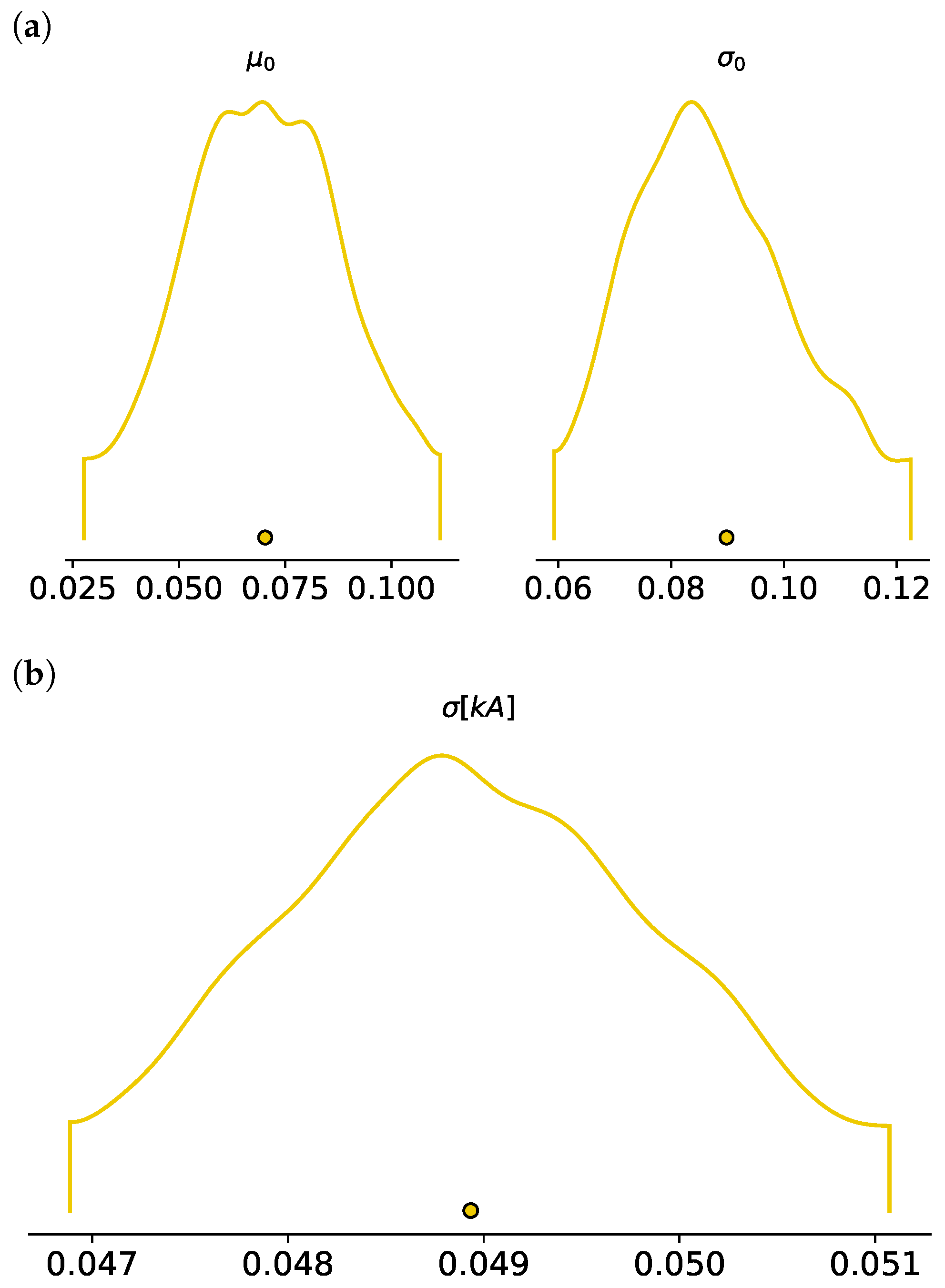
 [Green Version]
Figure 1. Graphical representation of parameters in Bayesian model for functional representation of the signal. Spline weights θ m come from the normal distribution with hyper-parameters μ 0 and σ 0 . Those parameters are inferred in the hierarchical way from data with uniform hyper-priors. Measurements y n are disturbed by a zero mean Gaussian noise with standard deviation of σ .
Energies 14 05893 g001
Figure 2. Circuit diagrams of simulated cable faults in VSC DC systems: (a) Pole-to-pole short circuits. (b) Pole- to-ground short circuits. For those faults Mesas et al. [9] have provided simulation models using solutions of differential equations. x—location of fault, L x —distributed inductance, R x —distributed resistance, C—capacitance of DC link capacitor, R f —fault resistance, v c —DC-link capacitor voltage, i c a b l e —cable current, L c h o k e is the grid-side choke inductance, i g a , b , c —IGBT currents.
Energies 14 05893 g002
Figure 3. For algorithm verification we have used simulations of initial stages (5 ms) of faults of VSC DC cables. We have selected a set of parameters, which was then randomized with normal distribution with standard deviation equal to 10% of given parameter. Then we have simulated both currents and voltages. Subfigure (a) describes the pole-to-pole faults and (b) pole to ground faults.
Energies 14 05893 g003
Figure 4. We consider a spline base of 15 third order polynomials. They are all based on equidistant knots and are continuously differentiable except at the boundary.
Energies 14 05893 g004
Figure 5. Bayesian model of the current signal manages to capture some of the uncertainty. Plot (a) shows, that error bars for splines further from start are much thinner than initially. The ribbon plot (b) shows quantiles of simulated output values compared to point quantiles of data. As we can see there is an underestimation of uncertainty in the middle of the signal.
Energies 14 05893 g005
Figure 6. Kernel density estimators of (a) hyper-parameters μ0, σ0 (which have no units) and (b) standard error of current measurement (kA) also show reasonable sampling behavior. However, flat middle of μ0 distribution and ‘triangular’ shape of σ might suggest some issues.
Energies 14 05893 g006
Figure 7. Application of the algorithm to two samples, one of pole-to-pole and one of pole-to-ground faults. (a) Bayesian model has efficiently captured the shape of measurements. (b) Distribution of data depth shows good discrimination of pole-to-ground from the reference depth; however, isolated pole-to-pole fault is also much more shallow. It suggests that current is a poor diagnostic indicator in this case.
Energies 14 05893 g007
Figure 8. Bayesian model of the voltage signal gives better representation of the uncertainty than in the case of current. Plot (a) shows that error bars for splines further from the start are much thinner than initially. The ribbon plot (b) shows quantiles of simulated output values compared to point quantiles of data. As we can see there is an underestimation of uncertainty in the middle of the signal; however, initial and final quantiles are covered without overstepping the data.
Energies 14 05893 g008
Figure 9. Kernel density estimators of (a) hyper-parameters μ0, σ0 (which have no units) and (b) standard error of voltage measurement (kV) also show reasonable sampling behavior. All the distributions are reasonably normal-like.
Energies 14 05893 g009
Figure 10. Application of the algorithm to two voltage samples, one of pole-to-pole and one of pole-to-ground faults. (a) Bayesian model has efficiently captured the shape of measurements. (b) Distribution of data depth shows good discrimination of pole-to-ground from the reference depth. Isolated pole-to-pole fault is also shallower than reference but reasonably close. It suggests that voltage is a much better diagnostic indicator in this case.
Energies 14 05893 g010
Table 1. Hyper-prior parameters of the current spline model are efficiently estimated. They get very thin distributions centered in the neighborhood of zero. Standard error of the current measurement is estimated at 0.05 kA which is consistent with simulations. Probabilistic computation is efficient, as Monte Carlo standard error (MCSE) is vanishingly small. Effective sample size of both bulk of distribution and its tails is on the level of 42% (total numnber of samples is 4000) what is a reasonable result.
Meansdhdi_3%hdi_97%mcse_Meanmcse_sdess_Bulkess_Tailr_Hat
μ 0 0.0700.0220.0280.1120.0010.01686.01742.01.0
σ 0 0.0900.0180.0590.1230.0000.01687.01599.01.0
σ 0.0490.0010.0470.0510.0000.01689.02231.01.0
mean—mean value of variable, sd—standard deviation of variable, hdi_3%—bottom 3% of 94% best confidence interval, hdi_97%—top 3% of 94% confidence interval, mcse_mean—mean of Monte Carlo standard error for variable, mcse_sd—standard deviation of Monte Carlo standard error for variable, ess_bulk—effective sample size of samples from the bulk of distribution of variable, ess_tail—effective sample size of samples from the bulk of distribution of variable, r_hat—potential scale reduction factor R ^ .
Table 2. When analyzing current signal in the context of reference depth of pole-to-pole fault (with mean of 6.23 × 10 2 and spreading from 1.993 × 10 2 to 2.14 × 10 1 ) we can see that it is not the best indicator. While pole-to-ground scenarios are being clearly discriminated as ‘shallow’ with depths at the level of 10 5 , the pole-to-pole current signals are also separated from the reference not getting depths greater than 10 3 .
Pole-to-Pole FaultsPole-to-Ground Faults
MeanMinMaxMeanMinMax
Exp. no.
08.947 × 10 4 8.868 × 10 4 9.028 × 10 4 3.738 × 10 5 3.727 × 10 5 3.751 × 10 5
12.531 × 10 3 2.485 × 10 3 2.575 × 10 3 4.732 × 10 5 4.712 × 10 5 4.752 × 10 5
21.795 × 10 3 1.775 × 10 3 1.817 × 10 3 4.460 × 10 5 4.436 × 10 5 4.481 × 10 5
34.183 × 10 4 4.156 × 10 4 4.208 × 10 4 2.772 × 10 5 2.766 × 10 5 2.777 × 10 5
42.590 × 10 4 2.579 × 10 4 2.602 × 10 4 2.645 × 10 5 2.639 × 10 5 2.650 × 10 5
52.632 × 10 4 2.620 × 10 4 2.645 × 10 4 4.359 × 10 5 4.349 × 10 5 4.369 × 10 5
62.432 × 10 3 2.394 × 10 3 2.467 × 10 3 3.290 × 10 5 3.282 × 10 5 3.300 × 10 5
73.642 × 10 4 3.618 × 10 4 3.662 × 10 4 8.290 × 10 5 8.230 × 10 5 8.347 × 10 5
83.198 × 10 3 3.141 × 10 3 3.260 × 10 3 3.570 × 10 5 3.560 × 10 5 3.580 × 10 5
92.255 × 10 3 2.222 × 10 3 2.290 × 10 3 5.212 × 10 5 5.184 × 10 5 5.236 × 10 5
Exp. no.—experiment number, mean—mean value of data depth of candidate signal consisting of one type of faults (no unit), min—minimal value of data depth of candidate signal consisting of one type of faults (no unit), max—maximal value of data depth of candidate signal consisting of one type of faults (no unit).
Table 3. Hyper-prior parameters of the voltage spline model are also efficiently estimated but with more difficulty. They get very thin distributions centered in the neighbourhood of zero; however, all of them are positive. Standard error of the voltage measurement is estimated at 0.02 kV which is consistent with simulations. Probabilistic computation is efficient, as Monte Carlo standard error (MCSE) is vanishingly small. Effective sample size of both bulk of distribution and its tails is on the level between 15% and 25% (total number of samples is 4000), which is a reasonable result. Potential scale reduction factor R ^ is reasonably close to 1, indicating good mixing of Markov chains.
Meansdhdi_3%hdi_97%mcse_meanmcse_sdess_bulkess_tailr_hat
μ 0 0.0310.0110.0110.0510.00.0840.0987.01.00
σ 0 0.0440.0090.0290.0600.00.0742.0877.01.00
σ 0.0190.0000.0180.0200.00.0733.0634.01.01
mean—mean value of variable, sd—standard deviation of variable, hdi_3%—bottom 3% of 94% best confidence interval, hdi_97%—top 3% of 94% confidence interval, mcse_mean—mean of Monte Carlo standard error for variable, mcse_sd—standard deviation of Monte Carlo standard error for variable, ess_bulk—effective sample size of samples from the bulk of distribution of variable, ess_tail—effective sample size of samples from the bulk of distribution of variable, r_hat—potential scale reduction factor R ^ .
Table 4. When analyzing voltage signal in the context of reference depth of pole-to-pole fault (with mean of 6.223 × 10 2 and spreading from 2.108 × 10 2 to 2.135 × 10 1 ) we can see that it is a much better indicator than current. Pole-to-ground scenarios are being clearly discriminated as ‘shallow’ with depths at the level of 10 5 as in the previous case. The pole-to-pole current signals are also separated from the reference but their depths are even sometimes overlapping reference or are relatively close to it.
Pole-to-Pole FaultsPole-to-Ground Faults
MeanMinMaxMeanMinMax
Exp. no.
09.176 × 10 3 5.036 × 10 3 1.934 × 10 2 3.672 × 10 5 3.553 × 10 5 3.802 × 10 5
14.282 × 10 4 3.818 × 10 4 4.818 × 10 4 6.690 × 10 5 6.360 × 10 5 7.041 × 10 5
22.489 × 10 3 1.813 × 10 3 3.540 × 10 3 2.596 × 10 5 2.510 × 10 5 2.673 × 10 5
31.124 × 10 3 9.160 × 10 4 1.398 × 10 3 2.265 × 10 5 2.193 × 10 5 2.342 × 10 5
47.260 × 10 4 6.172 × 10 4 8.566 × 10 4 4.809 × 10 5 4.596 × 10 5 5.037 × 10 5
51.881 × 10 4 1.744 × 10 4 2.029 × 10 4 1.104 × 10 4 1.032 × 10 4 1.202 × 10 4
61.163 × 10 4 1.091 × 10 4 1.236 × 10 4 2.081 × 10 4 1.905 × 10 4 2.279 × 10 4
75.456 × 10 3 3.664 × 10 3 8.499 × 10 3 3.052 × 10 5 2.903 × 10 5 3.206 × 10 5
86.295 × 10 4 5.348 × 10 4 7.457 × 10 4 5.398 × 10 5 5.131 × 10 5 5.675 × 10 5
93.252 × 10 3 2.331 × 10 3 5.029 × 10 3 3.930 × 10 5 3.789 × 10 5 4.080 × 10 5
101.521 × 10 2 6.879 × 10 3 3.795 × 10 2 3.035 × 10 5 2.923 × 10 5 3.148 × 10 5
Exp. no.—experiment number, mean—mean value of data depth of candidate signal consisting of one type of faults (no unit), min—minimal value of data depth of candidate signal consisting of one type of faults (no unit), max—maximal value of data depth of candidate signal consisting of one type of faults (no unit).
Publisher’s Note: MDPI stays neutral with regard to jurisdictional claims in published maps and institutional affiliations.

