Design and Pinch Analysis of a GFT Process for Production of Biojet Fuel from Biomass and Plastics

Abstract

Environmental problems are frequently related to energy use, estimated to grow at 1.6% per year until 2035. The transport sector accounts for 30% of energy demand and aviation is growing around 2.6% per year. Thus, low-emissions policies promote the use of sustainable aviation fuels. This work simulates a gasification and Fischer-Tropsch process to obtain biojet fuel from biomass and plastic waste. Syngas obtained through cogasification is purified by amine scrubbing and subjected to a Fischer-Tropsch process to produce hydrocarbons, which are upgraded for optimal fuel properties. Pinch analysis is applied to minimize energy usage, while Rankine cycles and a cooling tower are designed to cover the demand of electricity and cooling water. Results show that mass yields of the process towards biofuels are 13.06%, with an output of 1697.45 kg/h of biojet fuel. Density, kinematic viscosity, pour and flammability points and the lower calorific value of the biojet fuel comply with the ASTM D7566 standard. Pinch analysis allows to reduce 41.58% and 100% of cooling and heating demands, respectively, using biomass as renewable energy for heating. Moreover, steam generation covers 38.73% of the required electricity. The produced biojet fuel emits 20.14 g_CO2eq/MJ and has a minimum selling price of 1.37 EUR/L.

1. Introduction

Energy is the engine of society and one of the fundamental pillars of human progress. Global energy usage has increased significantly thanks to the large-scale incorporation of fossil fuels [1], which has led to a significant increase in living standards. Today, fossil fuels are still the main source of energy used worldwide, accounting for approximately 90% of energy demand [2]. However, the use of these raw materials as an energy source is the cause of the main environmental problems affecting the planet (climate change) and, due to their geographic location, has caused conflicts based on energy dependence and geopolitical strategies. According to the United Nations, at least 40% of violent conflicts in the last 60 years are related to the exploitation of strategic resources [3].

Renewable energies represent an alternative to conventional energy sources and biomass stands out among them, due to its ubiquity, availability, and low polluting nature [4]. Due to the increase in the price of fossil fuels and materials (in the United States the price of petrol between 2000 and 2021 has risen from 1.52 to 2.26 USD/gal [5]), in recent years, biorefineries present an interesting alternative, being able to efficiently convert renewable raw materials into a wide range of marketable products of biological origin.

Besides, nowadays plastic waste is another major environmental problem [6,7], as it ends up as waste that accumulates in landfills or is dumped into the environment. Plastics are resistant to decomposition, which makes them very versatile, but they need hundreds of years to be degraded in nature [8,9], leading to their accumulation, especially in the seas and oceans [10].

Plastic waste is sometimes shipped from developed countries to other countries, mainly Asian countries, for recycling, as exporting becomes cheaper than treating it in situ [9]. These practices are against circular economy and pose a double environmental problem. Firstly because of the transport of these plastics, and secondly because of the recycling treatments they receive in the destination countries since the legislation on their treatment and environmental regulations are much less restrictive than in the countries from which they originate. The final disposal of plastic waste in Europe [8] is as follows: landfill (52%), export (19%), recycling (18%), and incineration (11%).

An interesting option to reduce plastic dumping and export [11,12], is to convert plastic waste into fuels for transport sector, where the search of alternative fuels is a priority. This sector currently accounts for approximately 30% of global primary energy demand [13,14], of which more than 95% is obtained through the consumption of petroleum products [15].

In this context, aviation is the fastest way of transport for long distances and it covers 10% of the energy demand in the transport sector [15]. The number of flights is currently growing at 2.6% per year worldwide [16] and, in the European Union (EU), are expected to grow at 1.9% per year to 2040 [17]. Current aviation engine technology and regulations do not allow the commercial-scale use of hydrogen and electricity as energy sources; therefore, although regulations prevent the use of biofuel blends with traditional paraffin to exceed 50% by volume [18], the main alternative is biojet fuel.

There are several theoretical and experimental studies on biojet fuel production [19,20], and literature reviews depending on the feedstock and processes used [21]. The gasification and Fischer-Tropsch process (GFT) is based on reaction mechanisms whose kinetics and thermodynamic analysis are well known for a wide range of feedstocks [22,23,24]. However, no previous studies have been found that simulate reaction kinetics for cogasification of biomass and plastics. Once syngas is obtained, the industry already has mature technologies to convert it into fuels, such as CO₂ purification with amines [25,26], hydrocarbon synthesis via Fischer-Tropsch process [27,28] and final improvement of biojet fuel properties by hydrocracking (upgrading) [29,30,31,32,33].

The aims of this study are: (i) To simulate a cogasification of residual plastics and biomass (analysing the plant location to obtain input feedstock mass flow) to produce biojet fuel via GFT process, consisting of six units: a gasification unit, two amine scrubbing units, two reaction units (Fischer-Tropsch and upgrading), and a separation unit. (ii) To design a heat exchanger network, using the pinch method to reduce the demand of utilities (heating steam and cooling water). (iii) To design Rankine cycles and cooling tower to satisfy, as far as possible, the demand for steam, electricity, and fresh water required by the plant. (iv) Finally, to assess the technical viability of the biojet fuel, estimating combustion properties and CO_2eq emissions.

2. Materials and Methods

2.1. Location and Feedstock

In relation to sustainable aviation fuel, Europe is the continent that is making the most significant commitment [34], given its CO₂ emission reduction targets and its dependence on fossil fuels from other countries. While the geographical location of the plant has little influence on its design, it can play an important role in the economic analysis. The biojet fuel plant is located in Spain, because it is one of the main agricultural producers [35] and, therefore, a promising biojet fuel producer from biomass waste blended with plastics.

Residual biomass: In Spain, straw is the most abundant residual lignocellulosic biomass of agricultural origin [36]. Specifically, in the province of Huesca, wheat and barley straw production amounts to 178,002 and 579,448 tonnes per year (t/year), respectively. Although the total utilisation of wheat and barley residues available in the province is optimistic, other types of residual lignocellulosic biomass are generated and must be considered. Therefore, the mass flow of this raw material is considered achievable.

Plastic waste: Spain produces 1.5 million tonnes of plastic waste per year, of which approximately 20% is exported to other countries [9]. In order to estimate the quantity and composition of the plastic used as raw material, the following assumptions are made:

• The amount of waste generated per inhabitant is homogeneous throughout Spain;
• The average composition of plastic waste is based on the type of polymers demanded in Europe [8];
• A total of 90% of the polyethylene (PE) and polypropylene (PP) that would be exported from the provinces of Huesca, Zaragoza, Navarra, and La Rioja are fed into the chemical process.

For a plant operating factor of 8000 h per year, the raw material quantity and composition by mass (wt%) are shown in

Table 1. Raw material summary [8,9,36].

	t/year	t/h	wt%	wt%
Barley straw	579,448.00	72,431	70	91	Biomass
Wheat straw	178,002.00	22,250	21
Polyethylene	48,869.67	6109	6	9	Plastic
Polypropylene	25,630.02	3204	3

:

2.2. Process Simulation and Thermodynamic Models

Aspen Plus and Aspen HYSYS v10 have been used to simulate the process. The amount of raw material and the ratio between lignocellulosic biomass and plastic is based on Table 1. The biomass components (cellulose, hemicellulose, and lignin [37,38,39,40]) are entered as user-defined compounds using their molecular structure [4] for the software to estimate their physical properties. The software already contains polyethylene and polypropylene in its “APV100 POLYMER” database, which is used to simulate the plastic properties.

Furthermore, Aspen Plus has been used to model the physical properties of biomass and plastic applying NRTL [41] as thermodynamic model. Mass balance calculation for the distribution of pyrolysis products has been carried out by using Microsoft Excel. The gasification reactor and downstream processes have been simulated via Aspen HYSYS: using NRTL for gasification (unit 1, see Figure 1), FT process and upgrading (units 3 and 4, see Figure 2) [42]; Acid Gas—Chemical Solvents for amine scrubbing (unit 2, see Figure 1 and unit 5, see Figure 3) [43], and SRK for product separation (unit 6, see Figure 3) [44].

2.3. Heat Integration and Utilities

Energy integration between process streams has been studied using pinch analysis, performed via Aspen Energy Analyzer v10 software. Then, Rankine cycles (unit 7) were designed using Peng-Robinson [45], in Aspen HYSYS to cover part of the electrical demand, using the surplus steam generated.

Finally, EBSILON Professional v14.2 software was used to simulate a cooling tower. This software allows us to calculate the mass balance and the electrical power required by the equipment.

2.4. Economic Analysis

Total investment was estimated by the percentage method [46], based on equipment and raw materials costs. Minimum selling price (MSP) of biojet fuel and coproducts is assessed considering an internal rate of return (IRR) of 9% [47].

3. Results

3.1. Process Flow Diagram (PFD)

The chemical process starts in unit 1, shown in Figure 1 (refer to Table S9 of Supplementary Information to see the complete list of streams and equipment in PFD), where biomass (S101) and plastic (S102) are introduced into a fluidised bed boiler to be gasified in an oxygen-poor atmosphere (S109) to produce syngas. Steam (S105) is introduced to adjust the amount of hydrogen (H₂) generated. On one hand, the syngas leaves the boiler (S112) and is transported to unit 2. On the other hand, ashes and part of the bed-forming solids are removed from the boiler (S110).

Syngas enters unit 2, shown in Figure 1, where it must be purified to reduce its concentration of carbon dioxide (CO₂), as it poisons the Fischer-Tropsch reactor catalyst. Water (H₂O) and other condensable compounds (S203) are first separated from the syngas in a flash chamber. Recovered water is taken to a treatment plant so that it can be reused in the process. Gases separated in this flash chamber (S202) are taken to an absorption column, where an aqueous solution of monoethanolamine (MEA) is used to absorb the CO₂, leaving at the bottom as rich amine (S208).

Rich amine is taken to a flash chamber (V-203) and a rectification tower (T-202), where the CO₂ is separated and emitted to the atmosphere (S218).

The regenerated amine, known as lean amine, leaves the distillation tower and is taken to a mixer, where its composition is adjusted by the introduction of water and fresh amine, conditioning it back to the absorption column (S206).

The purified gas stream leaves the absorption column at the top (S207) and is fed to a pressure swing adsorption (PSA) bed, where the ratio of H₂ to carbon monoxide (CO) is adjusted. The syngas (S226) is fed to unit 3, and the separated hydrogen (S225) to unit 4.

In unit 3, shown in Figure 2, syngas is brought to Fischer-Tropsch reactor operating conditions. In the reactor, syngas is transformed into water and straight-chain hydrocarbons (S305), which are transported to unit 4.

In unit 4, products obtained from unit 3 are taken to a 3-phase separator, where the gaseous products (S403) are sent to unit 5. The water generated is taken to the water treatment plant (S405), and the hydrocarbons (S404) to the upgrading reactor, to react with the hydrogen separated in the PSA of unit 2 (S225).

Final products are obtained in units 5 and 6. In unit 5 (see Figure 3), fuel gas from the three-phase separator of unit 4 (S403), with a high carbon dioxide content, is purified by procedures similar to those of unit 2. The purified gases (S503) are the final product.

Rich amine (S504) must be regenerated and, for this purpose, it enters a rectification column where CO₂ is separated and emitted to the atmosphere (S507). The lean amine leaves the equipment and is taken to a mixer where water and fresh amine are added in order to replace the losses produced in the unit and adjust its composition, before being recirculated to the absorption column.

Unit 6 consists of a set of columns that allow the separation of the different products obtained. These products are fuel gas (S610), petrol (S611), biojet fuel (S619), diesel (S627), and fuel oil (S629).

3.2. Chemical Process Design

3.2.1. Gasification (Unit 1)

Feedstock is fed into the gasification reactor, where the processes of pyrolysis, oxidation, and reforming take place. Pyrolysis is endothermic and starts at around 300 °C for biomass and 450 °C for plastic [22,48]:

Cellulose + Hemicellulose + Lignin	→	Gas + Tar + Char
Plastic	→	Gas + Tar

In the case of biomass, the gas stream is mainly composed by carbon monoxide, carbon dioxide, methane (CH₄), ethylene (C₂H₄), and hydrogen. Char fraction is composed of carbon (C), ash, extractables and other solids. The tar is made up of hydrocarbons with an average composition of C₁₀H₁₀ and oxygenated compounds with an average composition of C₆H₁₀O₃ [48].

In the case of plastics, the gas stream is considered to be composed of hydrogen, ethylene, and 1-butene (C₄H₈). The produced tar is of two types: primary tar, consisting of aromatic hydrocarbons equivalent to cyclohexane (C₆H₁₂), and secondary tar, consisting of olefins of average composition C₁₀H₂₀ [48].

Pyrolysis mechanism is very fast and usually considered to occur instantaneously. Thus, a mass distribution of compounds formed after pyrolysis at 600 °C is calculated using the following equation [48]:

$$\left(a_0+a_1·T+a_2·T^2+a_3·T^3\right),$$

(1)

where a₀, a₁, a₂, and a₃ are parameters from

Table 2. Distribution of pyrolysis products.

		a0	a1	a2	a3	Result (wt%) (1)
TarBiomass	C6H10O3	19	−0.1735	7.4 × 10−5	0	0.10
	C10H10	19	−0.1735	7.4 × 10−5	0	0.10
TarPlastic	--	2850	−11.1	1.44 × 10−2	−6.22·10−6	30.48
TarPrimary (2)	C6H12	87.037	−0.52287	6.1991·10−4	0	0.00
TarSecondary (3)	C10H20	--	--	--	--	30.48
CharBiomass	C	209	−0.347	1.48 × 10−4	0	0.19
Gas (4)	H2	26	−4.47 × 10−2	4.54· × 10−5	0	1.68 (5)
		−49.816	0.13572	−8.6478 × 10−5	0	0.31 (6)
	CO (5)	26	5.44 × 10−2	−3.88 × 10−5	0	48.59
	CO2 (5)	214	−0.353	1.55 × 10−4	0	42.27
	CH4	−45	0.112	−5.47 × 10−5	0	7.08 (5)
		1440.6	−3.75	2.4997 × 10−3	0	54.74 (6)
	C2H4	−132	0.251	−1.15 × 10−4	0	0.00 (5)
		−748.92	2.13	−1.4122 × 10−3	0	14.47 (6)
	C4H8 (6)	−529.15	1.4567	−9.7835 × 10−4	0	0.00

⁽¹⁾ Calculated for biomass and plastic separately. ⁽²⁾ Calculated as wt% of Tar_Plastic. ⁽³⁾ Calculated as the remaining Tar_Plastic. ⁽⁴⁾ Gas wt% is calculated as 100-wt%_Tar+Char. For biomass, results are obtained as a volumetric composition (vol%) of gas and reconverted to wt%. For plastic, results are obtained as a wt% of gas. ⁽⁵⁾ Equation parameters and results for biomass. ⁽⁶⁾ Equation parameters and results for plastic.

. Temperature (T) is expressed in K for biomass and in °C for plastic.

Average specific heat (c_p) and specific enthalpy (h) of the species involved in the pyrolysis have been obtained from Aspen Plus (see

Table 3. Mass flow, specific heat, and enthalpy of pyrolysis species.

	kg/s	cp (kJ/kg·K)	h600°C (kJ/kg)
Feedstock	28.9	0.35	--
Reactants	26.0	--	−224.7
Products		--	−4088.3

). The mass of reactants is the mass of feedstock minus extractables and ash of S101 (see mass balances in Supplementary Information Section A):

The heat required for pyrolysis reaction is calculated using the equation:

$$H_{Pyrolysis}={\dot{m}}_{Feedstock}·C_P·\left(\Delta T\right)+{\dot{m}}_{Reacting}·\left(H_{Products}-H_{Reactives}\right),$$

(2)

where ΔT is the temperature difference between the pyrolysis (600 °C) and the reference temperature (25 °C). The heat required for the reaction is 106 MW, which is the minimum heat to be released during gasification to make the reactor autothermal.

After pyrolysis, the gasification takes place, in which the compounds shown in Table 2 react with each other and the gasifying agent to form syngas. In this study, a sufficient amount of air is introduced so the exothermic mechanism of gasification compensates the endothermic mechanisms of pyrolysis and reforming [49,50].

The reactions that take place in gasification and their kinetics are as follows (r is the reaction rate (kmol/(m³·s)); the concentrations of referenced compounds are in kmol/m³; T (K); E_A is the activation energy (kJ/kmol) and p_O2, p_H2O is the partial pressure of O₂ and H₂O (Pa)):

• Oxidation of gaseous compounds [51]:

  $$\mathrm{CO}+0.5{\mathrm{O}}_2\leftrightarrow {\mathrm{CO}}_2,$$

  (R1)

  $$r={10}^{10}·e^{-\frac{526.68}{R·T}}·{\left[\mathrm{CO}\right]}^{0.5}·{\left[{\mathrm{O}}_2\right]}^{0.5}·{\left[{\mathrm{CO}}_2\right]}^{0.5},$$

  (3)

  $${\mathrm{H}}_2+0.5{\mathrm{O}}_2\to {\mathrm{H}}_2\mathrm{O},$$

  (R2)

  $$r={10}^{11}·e^{-\frac{1202.79}{R·T}}·\left[{\mathrm{H}}_2\right]·\left[{\mathrm{O}}_2\right],$$

  (4)

  $${\mathrm{CH}}_4+1.5{\mathrm{O}}_2\to \mathrm{CO}+2{\mathrm{H}}_2\mathrm{O},$$

  (R3)

  $$r=1.58\times {10}^{10}·e^{-\frac{2927.95}{R·T}}·{\left[{\mathrm{CH}}_4\right]}^{0.7}·{\left[{\mathrm{O}}_2\right]}^{0.8},$$

  (5)

  $${\mathrm{C}}_2{\mathrm{H}}_4+2{\mathrm{O}}_2\to 2\mathrm{CO}+2{\mathrm{H}}_2\mathrm{O},$$

  (R4)

  $$r=1.58\times {10}^{10}·e^{-\frac{2927.95}{R·T}}·{\left[{\mathrm{C}}_2{\mathrm{H}}_4\right]}^{0.7}·{\left[{\mathrm{O}}_2\right]}^{0.8},$$

  (6)

  $${\mathrm{C}}_4{\mathrm{H}}_8+4{\mathrm{O}}_2\to 4\mathrm{CO}+4{\mathrm{H}}_2\mathrm{O},$$

  (R5)

  $$r=6.04\times {10}^9·e^{-\frac{1804.19}{R·T}}·{\left[{\mathrm{C}}_4{\mathrm{H}}_8\right]}^{0.25}·{\left[{\mathrm{O}}_2\right]}^{1.5}.$$

  (7)
• Tar oxidation [48]:

  $${\mathrm{C}}_6{\mathrm{H}}_{10}{\mathrm{O}}_3+4{\mathrm{O}}_2\to 6\mathrm{CO}+5{\mathrm{H}}_2\mathrm{O},$$

  (R6)

  $$r=1.58\times {10}^{13}·e^{-\frac{2910.75}{R·T}}·\left[{\mathrm{C}}_6{\mathrm{H}}_{10}{\mathrm{O}}_3\right]·\left[{\mathrm{O}}_2\right],$$

  (8)

  $${\mathrm{C}}_{10}{\mathrm{H}}_{10}+7.5{\mathrm{O}}_2\to 10\mathrm{CO}+5{\mathrm{H}}_2\mathrm{O},$$

  (R7)

  $$r=9.2\times {10}^6·e^{-\frac{9650}{R·T}}·{\left[{\mathrm{C}}_{10}{\mathrm{H}}_{10}\right]}^{0.5}·\left[{\mathrm{O}}_2\right],$$

  (9)

  $${\mathrm{C}}_6{\mathrm{H}}_{12}+6{\mathrm{O}}_2\to 6\mathrm{CO}+6{\mathrm{H}}_2\mathrm{O},$$

  (R8)

  $$r=3.8\times {10}^7·e^{-\frac{5545}{R·T}}·\left[{\mathrm{C}}_6{\mathrm{H}}_{12}\right]·\left[{\mathrm{O}}_2\right],$$

  (10)

  $${\mathrm{C}}_{10}{\mathrm{H}}_{20}+10{\mathrm{O}}_2\to 10\mathrm{CO}+10{\mathrm{H}}_2\mathrm{O},$$

  (R9)

  $$r=6.04\times {10}^9·e^{-\frac{1804.19}{R·T}}·{\left[{\mathrm{C}}_{10}{\mathrm{H}}_{20}\right]}^{0.25}·{\left[{\mathrm{O}}_2\right]}^{1.5}.$$

  (11)
• Char oxidation [48]:

  $$2\mathrm{C}+{\mathrm{O}}_2\leftrightarrow 2\mathrm{CO},$$

  (R10)

  $$\mathrm{Direct} \hspace{1em}\hspace{1em}r=1.51\times {10}^6·e^{-\frac{108.67}{R·T}}·p_{{\mathrm{O}}_2},$$

  (12)

  $$\mathrm{Reverse}\hspace{1em}\hspace{1em}r=5.3\times {10}^5·e^{-\frac{125}{R·T}}·p_{{\mathrm{O}}_2}^{0.53},$$

  (13)

  $$\mathrm{C}+{\mathrm{CO}}_2\to 2\mathrm{CO},$$

  (R11)

  $$r=1.4\times {10}^{11}·e^{-\frac{182.6}{R·T}},$$

  (14)

  $$\mathrm{C}+{\mathrm{H}}_2\mathrm{O}\to \mathrm{CO}+{\mathrm{H}}_2,$$

  (R12)

  $$r=2.62\times {10}^8·e^{-\frac{237}{R·T}}·p_{{\mathrm{H}}_2\mathrm{O}}^{0.57}.$$

  (15)
• Reforming [48]:

  $$\mathrm{CO}+{\mathrm{H}}_2\mathrm{O}\leftrightarrow {\mathrm{CO}}_2+{\mathrm{H}}_2,$$

  (R13)

  $$\mathrm{Direct}\hspace{1em}\hspace{1em}\hspace{1em}r=2.78\times {10}^3·e^{-\frac{12.6}{R·T}}·\left[\mathrm{CO}\right]·\left[{\mathrm{H}}_2\mathrm{O}\right],$$

  (16)

  $$\mathrm{Reverse}\hspace{1em}\hspace{1em}r=0.07\times {10}^3·e^{-\frac{489.27}{R·T}}·\left[{\mathrm{CO}}_2\right]·\left[{\mathrm{H}}_2\mathrm{O}\right],$$

  (17)

  $${\mathrm{CH}}_4+{\mathrm{H}}_2\mathrm{O}\leftrightarrow {\mathrm{CO}}_2+3{\mathrm{H}}_2,$$

  (R14)

  $$r=3\times {10}^5·e^{-\frac{1804.19}{R·T}}·\left[{\mathrm{CH}}_4\right]·\left[{\mathrm{H}}_2\mathrm{O}\right].$$

  (18)

Once unit 4 (see Figure 2) has been simulated, the amount of steam to be introduced into the reactor to generate the hydrogen required is known to be 2600 kg/h. On the other hand, 38,200 kg/h of oxygen must be fed to make the reactor autothermal, producing 3.6 MW of heat that must be removed to maintain isothermal conditions.

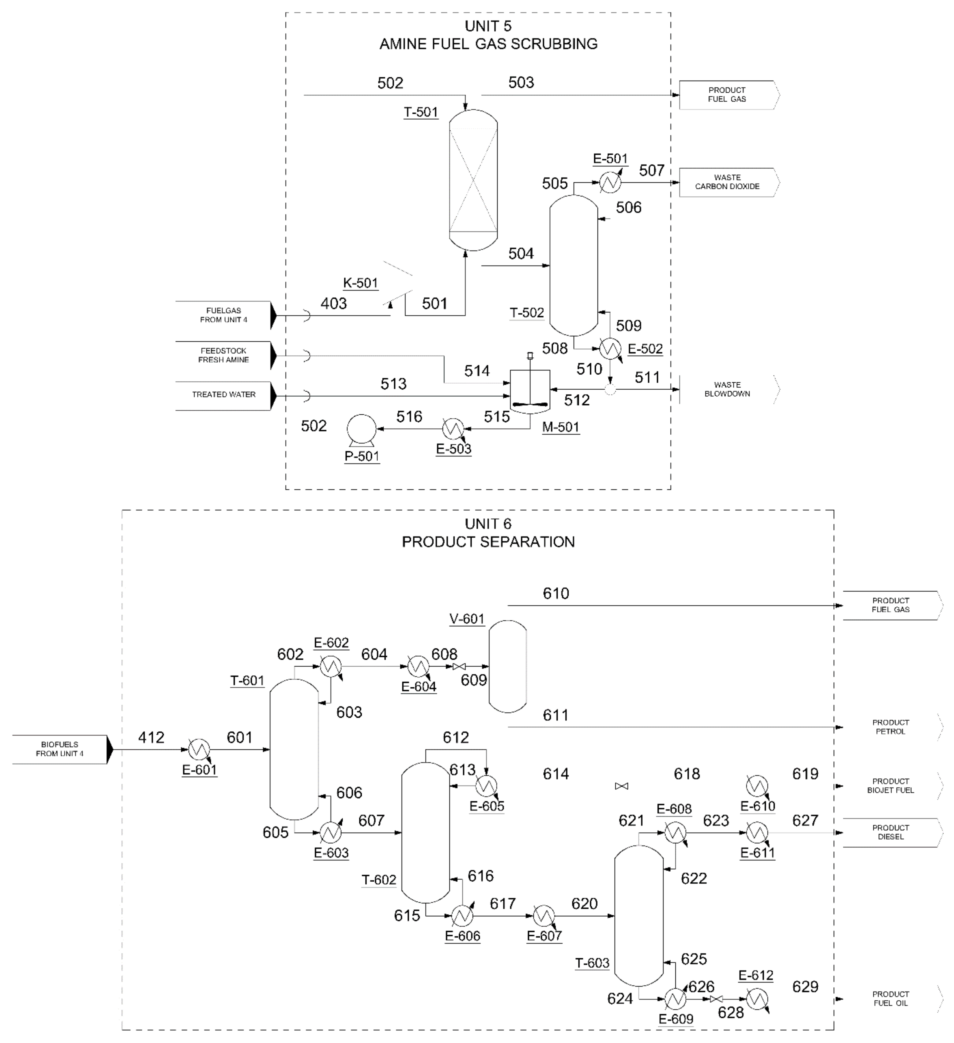
3.2.2. Amine Scrubbing (Units 2 and 5)

There are two streams with a high concentration of carbon dioxide: the syngas from gasification and the Fischer-Tropsch produced gas. The syngas obtained after gasification (S112, see Figure 1), with 70.4 wt%_CO2 that can poison the cobalt (Co) catalyst used in the Fischer-Tropsch (F-T) reactor [25]. On the other hand, the fuel gas obtained from F-T (S403, see Figure 3), with 62.4 wt%_CO2 reduces the calorific value of the stream.

MEA is selected as it requires a flow rate several orders of magnitude lower than other amines [26] for keeping CO₂ around 1 n/n% (mole percentage) in the clean gas stream. Before the recycle is introduced, the composition of the lean amine entering the absorption tower (S206/S502, see Figure 1 and Figure 3) is supposed to be 25 wt% of MEA and 2 wt% of CO₂. Next, the following parameters are adjusted in the absorption towers (T-201/T-501, see Figure 1 and Figure 3): contact stages, operating pressure, and temperature, and lean amine flow rate.

Increase of pressure improves the absorption and favours the formation of syngas. Thus, taking into account the pressure drop between R-101 (see Figure 1) and T-201, an operating pressure of 65 bar is selected for the absorber. In the case of T-501, the selected pressure is 3 bar, which is the maximum discharge pressure of K-501 compressor for which the gas temperature is less than 100 °C, as this would cause the water in the amine solution to boil.

Regarding the operating temperature, absorption improves at low temperatures, so both absorption towers operate at a temperature of 50 °C. Absorbers (T-201/T-501, see Figure 1 and Figure 3) are designed with 15 and 10 stages, respectively, to obtain less than 1 vol%_CO2 in the clean gas.

In unit 2, a flash chamber (V-203, see Figure 1) can be used for CO₂ separation, because there is a large pressure difference between the absorption tower and the regeneration tower (operating at a pressure of 2 bar). This separates 22.5 wt% of the CO₂ (S210).

Regeneration towers (T-202/T-502, see Figure 1 and Figure 3) operate at atmospheric pressure in the condensers and at 2 bar in the reboilers. These towers are designed for high CO₂ and amine recovery while avoiding high reflux and vaporisation ratios in both condenser and reboiler.

Condensers of all rectification towers in the plant operate at full reflux and temperatures higher than 50 °C, so water from cooling tower can be used for refrigeration.

Table 4. Main parameters of the regeneration towers (T-202/T-502).

	T-202	T-502
Stages	30	15
TCondenser (°C)	70	102
TReboiler (°C)	122	124
PCondenser (bar)	1.013	1.71
PReboiler (bar)	2.00	2.00
Reflux ratio	0.75	1.00

lists the main operating parameters of the regeneration towers:

In the amine syngas scrubbing unit (unit 2, see Figure 1), 98 n/n% of the carbon dioxide is recovered in the distillate, while 100 mol% of amine and 75 mol% of water are recovered in the residue. Sufficient water is generated in the process to replace these losses, so reducing the operating costs in the column is preferable to having a higher water recovery. The separated carbon dioxide (S214) is combined with the carbon dioxide obtained in V-203 (S210) and emitted to the atmosphere (S218). In the case of the amine fuel gas scrubbing unit (unit 5, see Figure 3), the carbon dioxide released is emitted directly.

After the regeneration towers, fresh water (S222/S513) and amine (S221/S514) are added in order to adjust the lean amine flow rate and composition. Then, lean amine (S206/S502) is conditioned and sent back to the absorption tower (T-201/T-501).

Following the absorption tower in unit 2, the clean syngas (S207) is sent to a PSA (V-202A/B, see Figure 1) which is used, on the one hand, to separate part of the hydrogen that is fed to the upgrading reactor (S225) and, on the other hand, to adjust the ratio of carbon monoxide to hydrogen in the syngas (S226) that is sent to the Fischer-Tropsch reactor.

3.2.3. Fischer-Tropsch Process (Unit 3)

The mass distribution of products obtained from this process (defined by Equation (19)) is calculated by the term “chain growth probability” (α) [28], which is a function of the type of catalyst used and the reaction conditions.

$$wt{\%}_{C_n}=\left[n·{\alpha }^{n-1}·{\left(1-\alpha \right)}^2\right]·100,$$

(19)

where n is the carbon number in the paraffin formed [52]. The chain growth probability must be iterated in order to maximise the production of biojet fuel, as it determines whether the hydrocarbons formed are light or heavy.

Once 0.88 has been obtained as the optimal α value, the results obtained are summarised in Figure 4, where the “Products” series has been obtained by applying Equation (19). The width of rectangles in “Fractions” series resembles the carbon number of hydrocarbons considered to be contained in each fraction (C₈–C₁₆ for biojet fuel) and their height is the sum of the mass distribution of the hydrocarbons contained (44.76 wt% of biojet fuel).

Reactions that take place for the production of straight-chain paraffins are:

$$n\mathrm{CO}+\left(2n+1\right){\mathrm{H}}_2\to {\mathrm{C}}_n{\mathrm{H}}_{2n+2}+n{\mathrm{H}}_2\mathrm{O}.$$

(R15)

Therefore, combining the probabilities of obtaining each hydrocarbon with the stoichiometry of each reaction, it is possible to calculate the optimal H₂/CO mole ratio, which has been determined at 2.08.

The operating temperature of the reactor is calculated taking into account the partial pressure of each species in the reactor, as shown in Equation (20):

$$\alpha =\left[1-0.039·\left(T-533\right)\right]·\left[0.2332·{\left(\frac{n_{{\mathrm{H}}_2}}{n_{\mathrm{CO}}}\right)}_{opt}+0.663\right],$$

(20)

where ${\left(\frac{n_{{\mathrm{H}}_2}}{n_{\mathrm{CO}}}\right)}_{opt}$ is the optimal H₂/CO mole ratio in the syngas. Therefore, the optimum operating temperature is 211 °C.

Mass composition of products from the Fischer Tropsch reactor (R-301, see Figure 2) is given in

Table 5. Composition of S305 (see Figure 2).

Compound	wt%	Compound	wt%	Compound	wt%
H2O	53.93	C8H18	1.62	C17H36	2.29
CO2	3.63	C9H20	1.80	C18H38	2.26
CH4	0.07	C10H22	1.95	C19H40	2.21
C2H4	0.12	C11H24	2.08	C20H42	2.15
C2H6	0.23	C12H26	2.17	C21H44	2.09
C3H8	0.45	C13H28	2.24	C22H46	2.02
C4H10	0.69	C14H30	2.28	C23H48	1.94
C5H12	0.94	C15H32	2.31	C24H50	1.86
C6H14	1.19	C16H34	2.31	C25H52	1.77
C7H16	1.41

:

Finally, using the enthalpy of the inlet and outlet streams and eliminating the sensible heat term in Equation (2), the heat given off in the reactor is estimated as 51 MW, which must be removed to maintain isothermal conditions.

3.2.4. Upgrading (Unit 4)

Linear hydrocarbons are taken to the upgrading reactor, where hydrocracking and isomerization take place, increasing the yield of light products and improving their properties for their commercialisation [53].

Inside the reactor, operating at 250 °C and 30 bar, the following reactions (with the correspondent mass yield η) occur [29]:

• Hydrocracking:

  $$\mathsf{\eta }=5.8\%\hspace{1em}\hspace{1em}{\mathrm{C}}_{13}{\mathrm{H}}_{28}+{\mathrm{H}}_2\to {\mathrm{C}}_{10}{\mathrm{H}}_{22}+{\mathrm{C}}_3{\mathrm{H}}_8,$$

  (R16)

  $$\mathsf{\eta }=61.7\%\hspace{1em}\hspace{1em}{\mathrm{C}}_{14}{\mathrm{H}}_{30}+{\mathrm{H}}_2\to {\mathrm{C}}_{11}{\mathrm{H}}_{24}+{\mathrm{C}}_3{\mathrm{H}}_8,$$

  (R17)

  $$\mathsf{\eta }=51.3\%\hspace{1em}\hspace{1em}{\mathrm{C}}_{15}{\mathrm{H}}_{32}+{\mathrm{H}}_2\to {\mathrm{C}}_{12}{\mathrm{H}}_{26}+{\mathrm{C}}_3{\mathrm{H}}_8,$$

  (R18)

  $$\mathsf{\eta }=37.1\%\hspace{1em}\hspace{1em}{\mathrm{C}}_{16}{\mathrm{H}}_{34}+{\mathrm{H}}_2\to {\mathrm{C}}_{13}{\mathrm{H}}_{28}+{\mathrm{C}}_3{\mathrm{H}}_8,$$

  (R19)

  $$\mathsf{\eta }=50.4\%\hspace{1em}\hspace{1em}{\mathrm{C}}_{17}{\mathrm{H}}_{36}+{\mathrm{H}}_2\to {\mathrm{C}}_{14}{\mathrm{H}}_{30}+{\mathrm{C}}_3{\mathrm{H}}_8,$$

  (R20)

  $$\mathsf{\eta }=4.9\%\hspace{1em}\hspace{1em}{\mathrm{C}}_{18}{\mathrm{H}}_{38}+{\mathrm{H}}_2\to {\mathrm{C}}_{15}{\mathrm{H}}_{32}+{\mathrm{C}}_3{\mathrm{H}}_8,$$

  (R21)

  $$\mathsf{\eta }=17.3\%\hspace{1em}\hspace{1em}{\mathrm{C}}_{17}{\mathrm{H}}_{36}+{\mathrm{H}}_2\to {\mathrm{C}}_9{\mathrm{H}}_{20}+{\mathrm{C}}_8{\mathrm{H}}_{18},$$

  (R22)

  $$\mathsf{\eta }=41.9\%\hspace{1em}\hspace{1em}{\mathrm{C}}_{18}{\mathrm{H}}_{38}+{\mathrm{H}}_2\to {\mathrm{C}}_{10}{\mathrm{H}}_{22}+{\mathrm{C}}_8{\mathrm{H}}_{18},$$

  (R23)

  $$\mathsf{\eta }=2\%\hspace{1em}\hspace{1em}{\mathrm{C}}_{17}{\mathrm{H}}_{36}+{\mathrm{H}}_2\to {\mathrm{C}}_{10}{\mathrm{H}}_{22}+{\mathrm{C}}_7{\mathrm{H}}_{16},$$

  (R24)

  $$\mathsf{\eta }=13.9\%\hspace{1em}\hspace{1em}{\mathrm{C}}_{18}{\mathrm{H}}_{38}+{\mathrm{H}}_2\to {\mathrm{C}}_{11}{\mathrm{H}}_{24}+{\mathrm{C}}_7{\mathrm{H}}_{16},$$

  (R25)

  $$\mathsf{\eta }=18\%\hspace{1em}\hspace{1em}\hspace{1em}\hspace{1em}{\mathrm{C}}_{16}{\mathrm{H}}_{34}+{\mathrm{H}}_2\to 2{\mathrm{C}}_8{\mathrm{H}}_{18},$$

  (R26)

  $$\mathsf{\eta }=23.2\%\hspace{1em}\hspace{1em}\hspace{1em}\hspace{1em}{\mathrm{C}}_{18}{\mathrm{H}}_{38}+{\mathrm{H}}_2\to 2{\mathrm{C}}_8{\mathrm{H}}_{20}.$$

  (R27)
• Isomerization:

  $$\mathsf{\eta }=90\%\hspace{1em}\hspace{1em}n-{\mathrm{C}}_8{\mathrm{H}}_{18}\to i-{\mathrm{C}}_8{\mathrm{H}}_{18},$$

  (R28)

  $$\mathsf{\eta }=88\%\hspace{1em}\hspace{1em}n-{\mathrm{C}}_9{\mathrm{H}}_{20}\to i-{\mathrm{C}}_9{\mathrm{H}}_{20},$$

  (R29)

  $$\mathsf{\eta }=90\%\hspace{1em}\hspace{1em}n-{\mathrm{C}}_{10}{\mathrm{H}}_{22}\to i-{\mathrm{C}}_{10}{\mathrm{H}}_{22},$$

  (R30)

  $$\mathsf{\eta }=90\%\hspace{1em}\hspace{1em}n-{\mathrm{C}}_{11}{\mathrm{H}}_{24}\to i-{\mathrm{C}}_{11}{\mathrm{H}}_{24},$$

  (R31)

  $$\mathsf{\eta }=90\%\hspace{1em}\hspace{1em}n-{\mathrm{C}}_{12}{\mathrm{H}}_{26}\to i-{\mathrm{C}}_{12}{\mathrm{H}}_{26},$$

  (R32)

  $$\mathsf{\eta }=90\%\hspace{1em}\hspace{1em}n-{\mathrm{C}}_{13}{\mathrm{H}}_{28}\to i-{\mathrm{C}}_{13}{\mathrm{H}}_{28},$$

  (R33)

  $$\mathsf{\eta }=53.9\%\hspace{1em}\hspace{1em}n-{\mathrm{C}}_{14}{\mathrm{H}}_{30}\to i-{\mathrm{C}}_{14}{\mathrm{H}}_{30},$$

  (R34)

  $$\mathsf{\eta }=27.2\%\hspace{1em}\hspace{1em}n-{\mathrm{C}}_{15}{\mathrm{H}}_{32}\to i-{\mathrm{C}}_{15}{\mathrm{H}}_{32},$$

  (R35)

  $$\mathsf{\eta }=6\%\hspace{1em}\hspace{1em}n-{\mathrm{C}}_{16}{\mathrm{H}}_{34}\to i-{\mathrm{C}}_{16}{\mathrm{H}}_{34},$$

  (R36)

  $$\mathsf{\eta }=12.6\%\hspace{1em}\hspace{1em}n-{\mathrm{C}}_{17}{\mathrm{H}}_{36}\to i-{\mathrm{C}}_{17}{\mathrm{H}}_{36},$$

  (R37)

  $$\mathsf{\eta }=18.9\%\hspace{1em}\hspace{1em}n-{\mathrm{C}}_{18}{\mathrm{H}}_{38}\to i-{\mathrm{C}}_{18}{\mathrm{H}}_{38}.$$

  (R38)

The amount of remaining reactants and formed products are estimated from mass yields and stoichiometric ratio of the different reactions. It is assumed that all isoparaffins formed have a single branch, with the methyl group on the second carbon of the chain [30,31,32,33,54,55].

Finally, using Equation (2) for the upgrading reactor (R-401, see Figure 2), the heat that must be removed to maintain isothermal conditions is estimated as 196 kW.

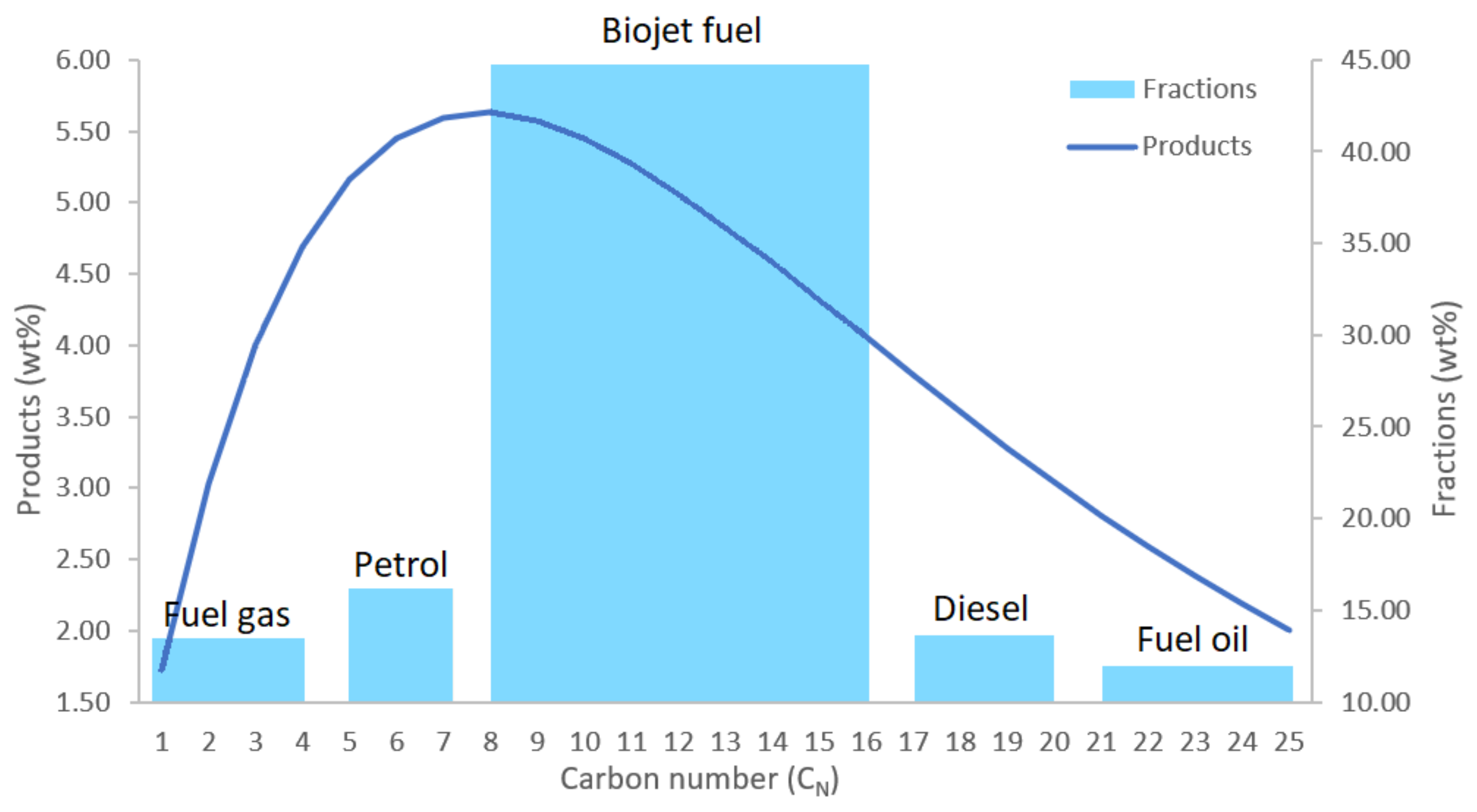
3.2.5. Product Separation (Unit 6)

The objective of the unit is to maximise the biojet fuel fraction, which comprises hydrocarbons from C₈ to C₁₆. However, n-octane (n-C₈) and isooctane (i-C₈) improve the properties of petrol, which contains hydrocarbons from C₅ to C₁₁. Therefore, in the first column (T-601, see Figure 3) the aim is to recover n-C₇, which forms part of the petrol, and n-C₉, which forms part of the biojet fuel (both are set to 99.5 n/n%). Under these conditions, the column has a certain flexibility of operation in which 90.7 n/n% of the C₈ is obtained in the distillate.

Light fractions are led to a flash chamber (V-601) to separate petrol from fuel gas, while heavier hydrocarbons are taken to two other rectification towers (T-602 and T603). T-602 is used to separate the biojet fuel from the heavier compounds; so, the recovery of i-C₁₆ in the distillate and n-C₁₇ in the residue is close to 100 n/n%. Finally, T-603 is used to separate diesel (C₁₅–C_20/25) from fuel oil (C₂₀₊), setting the recovery of n-C₁₉ (head) and n-C₂₁ (bottom) at 90 n/n%.

Table 6. Main parameters of the rectification columns (T-601/T-602/T-603, see Figure 3).

	T-601	T-602	T-603
Stages	25	25	30
TCondenser (°C)	135	252	349
TReboiler (°C)	305	438	438
PCondenser (bar)	4.00	5.00	1.71
PReboiler (bar)	6.00	2.50	3.50
Reflux ratio	1.15	1.30	2.90

lists the main parameters of the rectification columns:

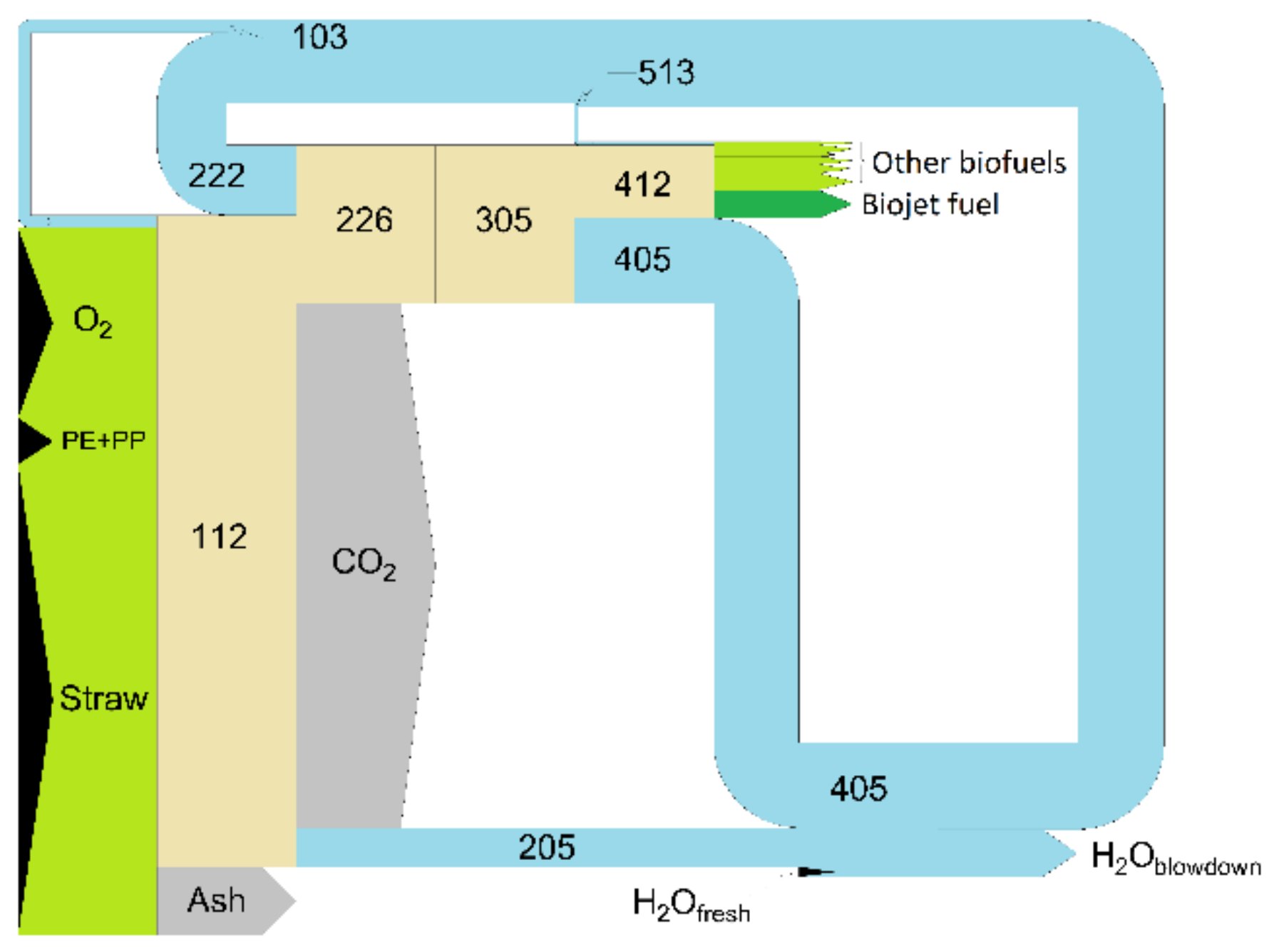
3.2.6. Overall Mass Balance

The mass flow between units is shown in Figure 5 and

Table 7. Overall mass balance.

Stream	kg/h	Stream	kg/h
Straw	94,681	S405	17,160
PE + PP	9312	S408	24
S103	2600	S412	12,940
O2	38,200	S503	646
Ash	13,753	S507	1936
S112	130,959	S511	0
S205	7843	S513	780
CO2	105,337	S514	0
S219	2	Other Biofuels (1)	561
S221	1		1590
S222	14,094		1697
S225	45		3416
S226	31,831	Biojet fuel	5676
S305	31,880	H2Ofresh	1991
S403	1802	H2Oblowdown	7742

⁽¹⁾ Fuel gas (S503 + S602), petrol (S611), diesel (S627) and fuel oil (S629), see SI E-F for detailed information.

(see Figure 1, Figure 2 and Figure 3 for stream identification):

As shown, 103,994 kg/h of biomass and plastic are used as raw material, which is converted into 1207 kg/h of fuel gas, 1590 kg/h of petrol, 5676 kg/h of biojet fuel, 1697 kg/h of diesel, and 3416 kg/h of fuel oil, which means a yield of 13.06% towards products. This yield could be slightly improved by adjusting the supply of oxygen as a gasifying agent, since CO₂ production has been increased to make the reactor autothermal.

All mass balance data sheets of the chemical process can be found in Supplementary Information Sections A–F.

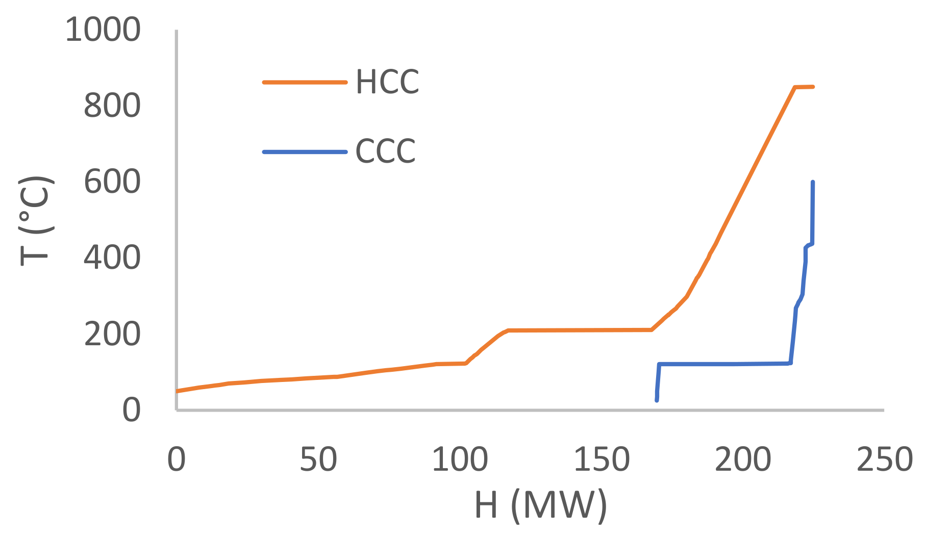
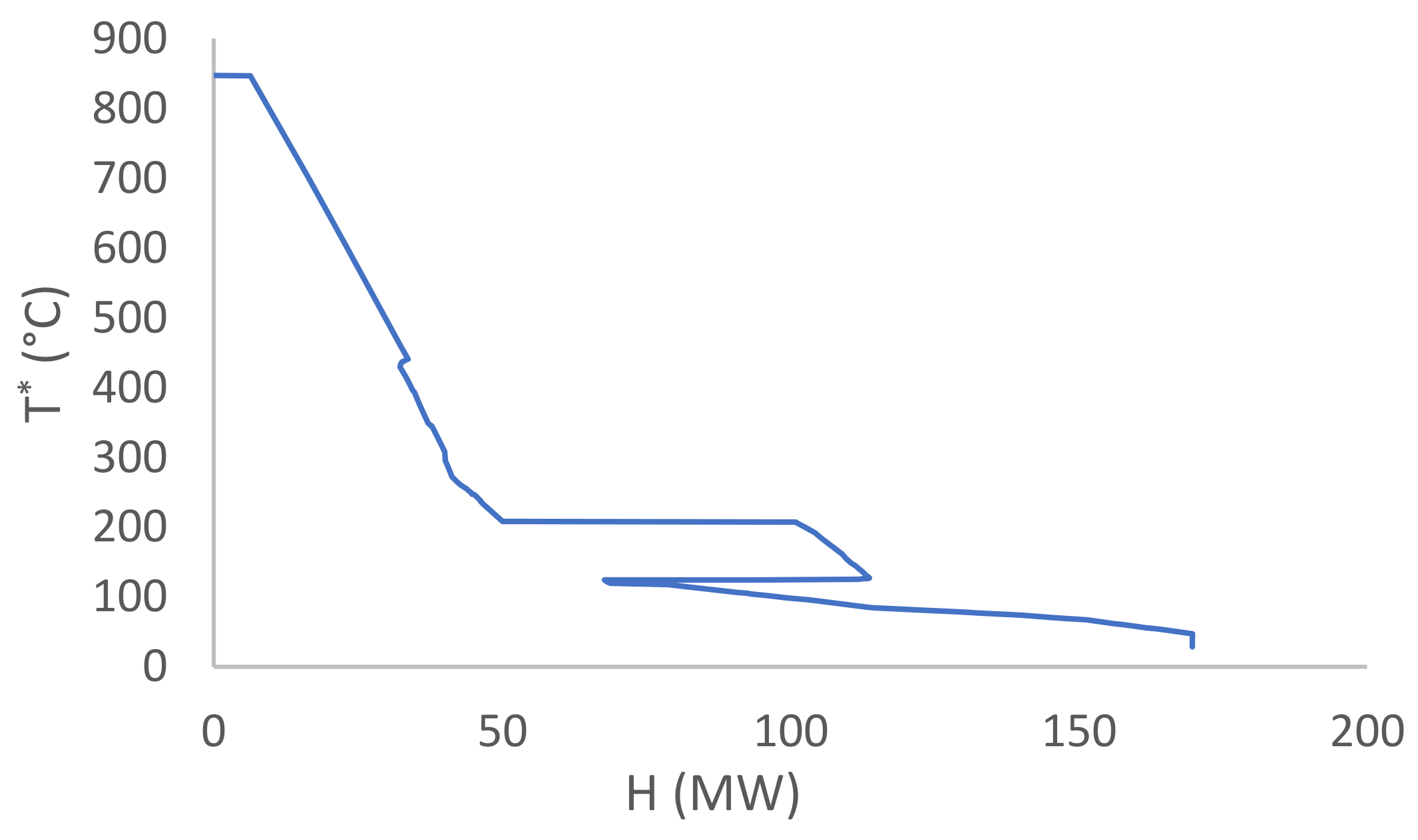
3.3. Heat Integration

Aspen Energy Analyzer is used to optimize energy demand. Stream properties were imported from Aspen HYSYS. The heat load released or given off by reactors, which require cooling or heating, is calculated for a difference of 1 °C from the operating temperature (see Supplementary Information Table S1). Prior to the pinch analysis, the heating and cooling demands are, respectively, 55,098 and 296,573 kW.

For the simulation of heat exchanger networks, Aspen Energy Analyzer allows the input of additional parameters such as viscosity (µ), thermal conductivity (k), and density (ρ), which have been obtained directly from Aspen HYSYS. These parameters and the flow velocity through the exchanger (v) are used to calculate the individual heat transfer coefficient of the fluid. This velocity is set to 15 m/s for gases and 3 m/s for liquids or phase changes (see Supplementary Information Table S2).

Hot streams, whose temperature need to decrease and require cooling, form the Hot Composite Curve (HCC). Cold streams, whose temperature need to increase and require heating, form the Cold Composite Curve (CCC). Plotting both curves in a T-H diagram (see Figure 6), there is a maximum approach, represented in green, which is given by the minimum admissible temperature difference (ΔT_min) in the heat exchangers [56]. This approach marks the optimal heating and cooling demands, from a thermodynamic point of view [57].

The design of the heat exchanger network and, therefore, the potential energy integration, implies the need to fix this minimum temperature difference (ΔT_min), so the heat exchanged is maximised without the size of equipment being excessive [58]. Using the Aspen Energy Analyzer software, the relationship between fixed and operating costs related to heat exchangers and utilities can be estimated, as shown in Figure 7:

Figure 6 shows that the whole CCC lies below the HCC, which means that there exists at least one heat exchanger network that fully satisfies the heating demand of the system. The excess heat from the process could be used for steam generation, which can be sold, so total costs shown in Figure 7 are negative, which indicate that the design of a heat exchanger network will have a positive impact on the economics of the project, which is an improvement to the GFT process. A ΔTmin of 6 °C is selected as economically optimal (see Figure 7) [57].

Once the ΔTmin is selected, the Grand Composite Curve (GCC) is drawn in Figure 8. The GCC allows to know pinch temperature (847 °C), and thermodynamically optimal demands (0 MW for heating and 170 MW for cooling):

In addition, the GCC is used to select the utilities for the heat exchanger network, as shown in

Table 8. Utilities for the heat exchanger network.

	Utility	Conditions at Heat Exchanger Inlet	Conditions at Heat Exchanger Outlet
For heating	Very high-pressure steam (HHPS)	Saturated steam at 260 °C	Saturated liquid at 259 °C
	High-pressure steam (HPS)	Saturated steam at 250 °C	Saturated liquid at 249 °C
For cooling (1)	Very high-pressure steam generation	Saturated liquid at 259 °C	Superheated steam at 270 °C
	High-pressure steam generation	Saturated liquid at 249 °C	Superheated steam at 260 °C
	Medium-pressure steam (MPS) generation	Saturated liquid at 174 °C	Superheated steam at 185 °C
	Low-pressure steam (LPS) generation	Saturated liquid at 124 °C	Superheated steam at 135 °C
	Water from cooling tower	Subcooled liquid at 28 °C	Subcooled liquid at 42 °C

⁽¹⁾ Given the high temperatures, it is possible to have steam generation. Steam is superheated 10 °C to avoid condensation during transport due to heat losses, so this heat is assumed to be dissipated.

:

Thus, knowing the demands, flow rates and properties of all streams and temperature of utilities, the heat exchange network is designed using the Aspen Energy Analyzer software (see Supplementary Information Figure S10).

The steam demanded by the cold streams is generated from the hot streams, so that the final heating and cooling demands of the chemical process are set at 173 MW for cooling (2.12% higher than the optimal) and 0 kW for heating; thus, the network manages to reduce the initial demands by 41.58 and 100%, respectively. By oversizing the necessary cooling water flow by 10%, the required mass flow rate of this utility is 6,830,113 kg/h.

3.4. Thermodynamic Cycles and Cooling Tower

3.4.1. Thermodynamic Cycles (Unit 7)

The excess steam generation, obtained from the heat exchanger network, is used to partially cover the electricity demand of the plant, calculated as 26,146 kW (see Supplementary Information Section L and unit 8 electricity demands in Section 3.4.2. Aspen HYSYS is used to design the different Rankine cycles for each steam pressure.

All cycles start in a heat exchanger where steam is generated (E-950, E-G_HPS, E-G_MPS and E-949, see Figure 9). This steam is taken, if required, to the heat exchanger network (E-939, E-952) and pumped (P-701, P-703) to the operating pressure of steam generators.

The rest of the steam is used to generate electricity in the turbines (ST-701, ST-702, ST-703, ST-704), cooled in the condensers (E-701, E-702, E-703, E-704), pumped (P-702, P-704, P-705, P-706) to the operating pressure of steam generators and sent to the heat exchanger network, closing the cycle.

Table 9. Inputs of the evaporators.

Cycle	Heat Exchanged (kW)	Evaporators
Very high-pressure steam	311	E-950
High-pressure steam	40,487	E-927, E-928, E-944, E-945 and E-951 (E-GHPS)
Medium-pressure steam	38,641	E-953 and E-954 (E-GMPS)
Low-pressure steam	312	E-949

shows heat used as an input for evaporators:

Likewise, the inlet and outlet temperatures for the steam at the different pressures are used as initial data: 259–270 °C for HHPS, 249–260 °C for HPS, 174–185 °C for MPS and 124–135 °C for LPS. For each steam type, the pressure at which evaporation occurs (at 260, 250, 175, and 125 °C respectively), is set at the steam outlet after the pressure drop in the evaporator.

In the high and very high-pressure cycles, flow dividers are used as part of the steam is sent for heating. A cooler is used to simulate 10 °C of temperature loss in transport. Moreover, exchangers that demand the steam are placed downstream, where the heat exchanged is introduced as an input, so that Aspen HYSYS can calculate the ratio of steam to be turbined and sent as utility.

The pressure drop in the turbine is limited so steam fraction at the turbine outlet is higher than 90%, or the outlet pressure higher than 0.4 bar.

Condensers (E-701, E-702, E-703, E-704, see Figure 9) use cooling water (CW) from the tower, so the inlet and outlet temperatures are assumed to be 28 and 42 °C, respectively. The data shown in

Table 10. Design of condensers for Unit 7.

Exchanger	HS (1)	TinHS (°C)	ToutHS (°C)	CS (2)	TinCS (°C)	ToutCS (°C)	H (kW)
E-701	HHPS	164	164	CW	28	42	254
E-702	HPS	153	152	CW	28	42	31,823
E-703	MPS	90	40	CW	28	42	33,191
E-704	LPS	76	71	CW	28	42	279

⁽¹⁾ Hot stream; ⁽²⁾ Cold stream.

and

Table 11. Design of condensers for Unit 7 (cont.).

Exchanger	U (kW/(m2·K))	LMTD (°C)	FT	S (m2)	SOvers. 10% (m2)	mCW (kg/h)
E-701	0.17	129	1.00	11.9	8.3	15,662
E-702	1.25	117	1.00	217.9	677.7	1,963,629
E-703	1.34	26	1.00	969.5	1066.5	2,048,032
E-704	0.15	38	1.00	48.9	24.1	17,210

are obtained after the simulation of the cooling tower (unit 8, see Figure 10):

Cooling water flow required by the cycle, oversized by 10%, reaches 4,448,986 kg/h, which is added to the 6,830,113 kg/h demanded by the chemical process, so that the total flow of water to be cooled by the cooling tower is 11,279,099 kg/h.

After simulating the cycles in Aspen HYSYS, the net power required is 10,431 kW, which means that the steam generated does not cover all the electrical demand of the chemical process equipment, so 16,698 kW must be purchased.

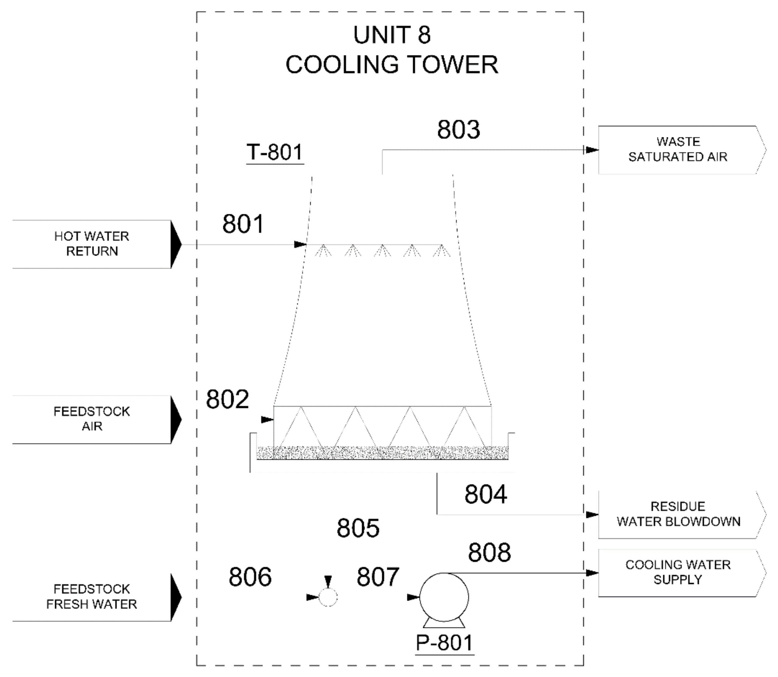
3.4.2. Cooling Tower (Unit 8)

This unit (see Figure 10) is simulated using Ebsilon Professional and a mechanical forced draft tower with countercurrent flow [59].

The hot water enters the cooling tower (S801, see Figure 10), is atomised, and then flows down. Air (S802), at ambient conditions, is introduced at the bottom and flows upwards, gets in contact with hot water and leaves the tower as saturated air (S803), cooling the liquid water, which falls into a pool at the bottom. The water losses increase the concentration of salts in the cycle over time, so part of the cooled water (S804) must be purged. The rest is recirculated (S805) and mixed with fresh water (S806) to make up for the losses, restarting the cycle.

Atmospheric pressure and a temperature of 25 °C for all raw materials are used as input. In addition, the average relative humidity of the air is assumed to be 75% [60]. Results of the cooling tower simulation are shown in

Table 12. Cooling tower results.

Water Flow to be cooled (kg/h)	11,279,099
Blowdown flow (kg/h)	53,932
Water makeup flow (kg/h)	270,230
TIn hot water (°C)	42
TOut cooled water (°C)	28
POvers. 10% (P-801) (kW)	343
POvers. 10% (fan) (kW)	641

:

The flow of fresh water taken from the medium represents approximately 3% of the refrigerated water flow. The mass balance data sheets of the thermodynamic cycles and the cooling tower can be found in SI G-H.

3.5. CO₂ Equivalent Emissions and Biojet Fuel Properties

On the one hand, emissions from biomass combustion are considered biogenic and not accounted in the biojet fuel life cycle. On the other hand, the gasification reactor is fed with 9 wt% of plastic waste (see Table 1), so 8227 kg/h of the carbon dioxide emitted has a non-renewable origin. These emissions are imputed to 13,586 kg of products; with an impact of 0.61 kg_CO2eq/kg_Biofuel. It should be noted that emissions could be reduced if the CO₂ captured from amine scrubbing were stored or transformed in different products [61].

In Spain, 0.2 t of carbon dioxide are emitted for each MWh demanded [62]. Thus, 0.25 kg_CO2eq/kg_Biofuel are caused by the usage of 16.7 MW of electricity. Taking into account a default value of 0.085 kg_CO2eq/(t·km) [63] for truck transportation (transport of the waste to the production plant and the fuel to the airports) and a distance of 200 km, transportation produces 0.02 kg_CO2eq/kg_Biofuel. The sum of CO₂ equivalent emissions is 0.9 kg_CO2eq/kg_Biofuel; which is considerably lower than in the case of conventional fuels [64], around 3 kg_CO2eq/kg_Fuel. (production) and 0.9 kg_CO2eq/kg_Fuel (consumption).

The low heating value of biojet fuel produced is 43.1 MJ/kg, therefore, around 20 g_CO2eq/MJ are emitted; complying with the 65% mandatory reduction stated in the European Directive 2018/2001 [65].

Biojet fuel properties are estimated using the analysis tools offered by Aspen HYSYS, to check whether it meets the requirements specified in ASTM D7566-20c standard [66]. Results are shown in

Table 13. Properties of biojet fuel compared to ASTM D7566 standard.

Parameter	GFT Biojet Fuel	ASTM D7566
Density at 15 °C (kg/m3)	742	730 to 770
Kinematic viscosity at −20 °C (cSt)	4	lower than 8
Pour point (°C)	−66	lower than −40
Flammability point (°C)	97	greater than 38
Lower calorific value (MJ/kg)	43.1	greater than 42.8

:

All estimated parameters comply with the standard. Other parameters (not estimated) could also comply, due to the nature of the fuel produced. Aromatic and naphthalene content is negligible, since the biojet fuel produced contains straight and branched chain hydrocarbons. Moreover, there is no sulphur (and, therefore, no mercaptan content), which together with water, acids, and carbon dioxide, is one of the main causes of corrosion and high electrical conductivity [67]. Distillation curve temperatures should also be met, since the hydrocarbons that make up the biojet fuel match those that make up conventional paraffin (see Figure 4). Finally, the smoke point requirement should not cause problems, since paraffins and isoparaffins (with higher H/C ratio than other hydrocarbons) reduce the amount of smoke produced [67].

Therefore, the estimated properties of the produced biojet fuel fulfill the standard. Experimental tests should be performed to ensure that it could be blended up to 50% with conventional jet fuel [66].

3.6. Economic Analysis

Fixed and variable costs are taken into account to estimate the minimum selling price of the biojet fuel produced and assess if the pinch analysis and the use of Rankine cycles makes the process economically more attractive.

3.6.1. Cost of Equipment

The cost the equipment is calculated using equations of

Table 14. Cost of equipment [46].

Equipment	Cost Equation (EUR)	Equation Number
Pumps (1)	$Cos{t}_{2007}=6900+206·V^{0.9}$	(21)
Compressors (2)	$Cos{t}_{2007}=\mathrm{490,000}+\mathrm{16,800}·P^{0.6}$	(22)
Heat exchangers (3)	$Cos{t}_{2007}=\mathrm{22,080}+46·S^{1.2}$	(23)
Furnace (4)	$Cos{t}_{2007}=\mathrm{180,000}·H$	(24)
Cooling tower (5)	$Cos{t}_{2007}=\mathrm{250,000}+1300·V^{0.9}$	(25)
Steam turbines (6)	$Cos{t}_{2007}=\mathrm{14,500}·P^{0.452}$	(26)

⁽¹⁾ V is the volumetric flow rate in L/s. The cost is doubled, as pumps are installed with a spare. ⁽²⁾ P is the power in kW. ⁽³⁾ S is the exchange surface in m². ⁽⁴⁾ H is the heat produced by F-101 in millions of kcal/h (9.45 million kcal/h). ⁽⁵⁾ V is the flow of water to be cooled (S801) in L/s. ⁽⁶⁾ P is the power generated in kW.

:

• Plastic and biomass feed hoppers and mixers:

They are calculated as vessels. A length to diameter (L/D) ratio of 5 gives the minimum cost. Applying Equation S3 (see SI L) and a residence time of 15 min, the hoppers volume can be calculated, which is oversized by 100%:

A total of 3 mm of corrosion allowance (C.A.), carbon steel as construction material, and a design pressure of 3.5 kg/cm² are used for the following calculations, as lean amine and raw materials are assumed to be non-corrosive:

$$D=\sqrt[3]{\frac{4·V}{\pi ·\left(\frac{L}{D}\right)}},$$

(27)

$$L=D·\left(\frac{L}{D}\right),$$

(28)

$$t=C.A.+P_D·\left(\frac{D}{2}\right)·\frac{1000}{St·E-0.6·P_D},$$

(29)

$$W=0.0246·D·\left(L+0.8·D\right)·\left(t+x\right),$$

(30)

$$Cos{t}_{2007}=\mathrm{13,014}·W^{0.92}·{\left(\frac{L}{D}\right)}^{-0.15}·{\left(\frac{t}{8}\right)}^{-0.21}.$$

(31)

where:

• D is the diameter of the vessel (m);
• V, volume (m³);
• L, lenght (m);
• t, thickness (mm);
• C.A., corrosion allowance (mm);
• P_D, the design pressure (kg/cm²);
• St, a dimensionless factor depending on the material, pressure and temperature conditions. This value is set to 1055 when using carbon steel and moderate conditions;
• E, modulus of elasticity of carbon steel, which is 0.85 GPa;
• W, weight of the equipment (t);
• X, a complexity factor, considered 2 for simple equipment;

• Flash chambers:

Thickness, mass, and cost of flash chambers are calculated using the following equations:

$$t=t_{Shell}+C.A.,$$

(32)

$$m=\pi ·\rho ·L·D·e,$$

(33)

$$Cos{t}_{2007}=\mathrm{10,000}+29·m^{0.85},$$

(34)

where data such as shell thicknesses (t_Shell), corrosion allowances, lengths, diameters, and densities of the materials have been obtained from Aspen HYSYS, using a liquid volume in the vessels of 50%.

• Distillation columns:

Their cost is calculated as the sum of vessel and trays cost:

$$Cos{t}_{Vessel 2007}=\mathrm{17,640}·D^{1.066}·L^{0.802},$$

(35)

$$Cos{t}_{Trays 2007}=0.92·\left(290+550·D^{1.9}·N_{Trays}\right).$$

(36)

Sections and heights are sized and trays are selected using Aspen HYSYS, so the fluid dynamics in each plate and all parameters are in a normal operating range. Columns are divided into sections and the cost is calculated as the sum of each individual section.

In addition, the installed cost of PSAs for oxygen (to be fed to F-101) and hydrogen purification (V-202A/B), and the R-301 and R-401 reactors, is calculated using the exponent (exp) method and their respective installation factors:

$$Cos{t}_{Installed}=0.92·F_{Installation}·Cos{t}_{Base}·{\left(\frac{Cap}{Ca{p}_{Base}}\right)}^{exp},$$

(37)

where the base capacities (Cap_Base) are the following [28]:

• For oxygen separation PSA, the air flow rate obtained (t/h);
• For hydrogen separation PSA, the flow rate of hydrogen separated (kg/h);
• For the Fischer-Tropsch reactor, the feed flow rate (kmol/h);
• For the upgrading reactor, the feed flow rate (kg/h).

The capacity (Cap) of the equipment and costs are shown in

Table 15. Cost of PSAs (V-202A/B, see Figure 1) and reactors (R-301/R-401, see Figure 2).

Equipment	CapBase	CostBase (USD)	Year	Exp	Cap	FInstallation	CostInstalled (EUR)
R-301	3186	10,500,000	2003	0.72	2955.4	1	9,151,283
R-401	4355	5,021,074	2011	0.65	12,940.0	3	28,126,803
PSAAir	24	24,552,000	2002	0.75	38.2	1	32,008,387
V-202A/B	8665	4,855,471	2002	0.6	44.8	2.47	468,393

:

For the rest of the equipment, the installation factor (F_Installation) is unique and is calculated from different factors, such as material (f_M, carbon steel), equipment placement (f_ER), piping cost (f_P), instrumentation and control (f_I), electricity (f_EI), civil works (f_C), buildings and structures (f_S), and thermal insulation and painting (f_L), whose values are 1, 0.3, 0.8, 0.3, 0.2, 0.3, 0.2, and 0.1 respectively [46].

To obtain the cost of installed equipment, the following equation is applied:

$$Cos{t}_{Installed}=Cos·\left[\left(1+Cost\right)·f_M+\left(f_{ER}+f_P+f_I+f_{EI}+f_C+f_S+f_L\right)\right].$$

(38)

The equipment costs are calculated and updated using the following expression, where the chemical plant cost index (CEPCI) of the year 2007 (former) is 525.4 and for 2018 (current) is 603.1 [45]:

$$Cos{t}_{Updated}=Cos{t}_{Installed}·\frac{CEPC{I}_{Current}}{CEPC{I}_{Former}}.$$

(39)

Table 16. Equipment costs.

Equipment	CostPurchase2007 (EUR)	CostInstalled2007 (EUR)	CostInstalled2018 (EUR)
Trays	485,804	485,804	557,649
Pumps	5,544,448	17,742,233	20,366,084
Compressors	10,840,115	34,688,369	39,818,339
Heat exchangers	2,384,730	7,631,136	8,759,684
Furnace	17,014,877	54,447,606	62,499,717
Hoppers and mixers	243,213	778,283	893,381
Flash chambers	296,036	947,314	1,087,410
Tower vessels	2,791,047	8,931,351	10,252,184
Cooling tower	2,071,034	6,627,309	7,607,404
Steam turbines	1,537,455	4,919,856	5,647,441
Total			253,468,920

lists the cost of all equipment:

3.6.2. Cost of Raw Materials and Products

Costs for cooling water (S806), process water (S001), fuel oil (S629), and electricity have been obtained for the year 2015, while that for biomass (S101) has been obtained for the year 2007, so they must be updated using Equation (47); knowing that the CEPCI for the year 2015 was 556.8 [68]. The material balance for the calculation of the fresh process water flow rate is calculated in Supplementary Information Section I.

Thus,

Table 17. Quantity and price of raw materials and products.

		Quantity	CostUpdated
Purchase	WaterProcess	1991 kg/h	2.06 × 10−4 EUR/kg
	WaterCooling	270,230 kg/h	2.06 × 10−5 EUR/kg
	Electricity	16,698 kWh	0.098 EUR/kWh
	Wheat straw	22,250 kg/h	0.037 EUR/kg
	Barley straw	72,431 kg/h	0.037 EUR/kg
	Poliethylene	6109 kg/h	0.02 EUR/kg
	Polipropylene	3204 kg/h	0.02 EUR/kg
	Amine	0.97 kg/h	1.40 EUR/kg
Sale	Fuel gas	1 m3/h	0.16 EUR/L (1)
	Petrol	2 m3/h	0.34 EUR/L (1)
	Biojet fuel	8 m3/h	0.39 EUR/L (1)
	Diesel	2 m3/h	0.42 EUR/L (1)
	Fuel oil	4 m3/h	0.24 EUR/L (1)

⁽¹⁾ Conventional fuel sale price.

is obtained [69]:

The cost of raw materials is 42,698,867 EUR/year and the amount obtained from the sale of products is 50,453,213 EUR/year.

3.6.3. Minimum Selling Price

The percentage method (see

Table 18. Percentage method.

Cost of Equipment (E)	253,468,921 EUR
	% of E	Cost (EUR)
Materials (M)	65	164,754,798
	% of E + M	Cost (EUR)
Detailed engineering (D.E.)	17.5	73,189,150
Licenses, process engineering… (P.E.)	--	1,500,000
Construction (Con.)	60	250,934,231
Construction supervision (Con.S.)	10	41,822,372
Inside battery limits (ISBL)	785,669,471 EUR
	% of ISBL	Cost (EUR)
Utilities (Ut.)	4	31,426,779
Off-sites (O.S.)	8	62,853,558
Start-up costs (S.C.)	3.5	27,498,431
Unforeseen contingencies (U.C.)	10	78,566,947
Fixed capital (F.C.)	986,015,186 EUR
Working capital (W.C.)	197,203,037 EUR

) is used to obtain a reference value for the fixed and working capital, based on the total cost of equipment [46]:

where [46]:

$$ISBL=E+M+D.E.+P.E.+Con.+Con.S,$$

(40)

$$F.C.=ISBL+Ut.+O.S.+S.C.+U.C.,$$

(41)

$$W.C.=0.2·C.I..$$

(42)

Engineering and construction works are assumed to last 3 years, in which the fixed capital is invested (20% first year, 50% second year, 30% last year), from years 0 to 2. Plant lifespan is 20 years, from years 3 to 22 and inflation is considered to be 4% per year. Thus, fixed capital is updated:

$$F.C{.}_{Updated}={\%}_{Invested}·F.C.·{\left(1+I\right)}^{Year}.$$

(43)

The working capital is invested at the end of the project in the third year at the updated cost, and that amount is recovered in year 22.

$$W.C{.}_{Updated}=W.C.·{\left(1+I\right)}^{Year},$$

(44)

$$T.I.=F.C{.}_{Updated}+W.C{.}_{Updated}.$$

(45)

During plant operation years, there is no investment, only the profits or losses from the sale and purchase of products and raw materials. In this scenario, 45 employees will be paid an average of 1800 EUR per worker [70], 1,134,000 EUR in total. Insurance is assumed to be 2% [46] of the fixed capital, 19,281,762 EUR. Both costs are added to the cost of raw materials to be purchased. These costs (C.) and sales profits (S.) are updated annually:

$$S{.}_{Updated}=S.·{\left(1+I\right)}^{Year},$$

(46)

$$C{.}_{Updated}=C.·{\left(1+I\right)}^{Year}.$$

(47)

During the first 10 years of plant operation, depreciation (D.) for the fixed capital invested in the project is accounted as:

$$D{.}_{Updated}=F.C.·\frac{I·{\left(1+I\right)}^{Year}}{{\left(1+I\right)}^{Year-1}}.$$

(48)

This depreciation has a value of 0 for the remaining years of operation, and allows tax deductions (T.), as these are calculated as 35% of the pre-tax profits (P.T.P.):

$$P.T.P.=C{.}_{Updated}-S{.}_{Updated}-D{.}_{Updated},$$

(49)

$$T.=0.35·P.T.P..$$

(50)

Profit after tax (P.A.T.) is calculated as the difference between profit before tax and tax. Finally, funds generated (F.G.) and cash flow (C.F.) are calculated:

$$P.A.T.=P.T.P.-T.,$$

(51)

$$F.G.=D{.}_{Updated}+P.A.T.,$$

(52)

$$C.F.=F.G.-T.I..$$

(53)

Results are shown in Supplementary Information Table S10.

From the cash flow obtained for each year, a sensitivity analysis is performed by taking each year’s cash flow and updating it for a chosen rate of return (RoR):

$$C.F{.}_{ Updated}=\frac{C.F.}{{\left(1+RoR\right)}^{Year}}.$$

(54)

The sum of cash flows gives the net present value (NPV) of the plant.

Bioproducts selling prices need to be higher than conventional petroleum fuels prices for the plant to be profitable. Thus, if an internal rate of return (IRR) of 9% is used, [47], bioproducts MSP are shown in

Table 19. MSP of biofuels for the studied process.

Product	MSP
	EUR/kg	EUR/L
Natural gas	0.51	0.54
Petrol	1.71	1.16
Biojet fuel	1.85	1.37
Diesel	1.90	1.45
Fuel oil	1.42	1.09

:

These prices are 3.47 times higher than conventional fuels prices (see Table 17), but similar to prices found in other studies for biojet fuel [18,21,28]. EU sets a tax of approximately 25 EUR/t_CO2eq [18] to penalise CO₂ emissions, which would increase the price of biojet fuel by around 0.02 EUR/kg, which increases the fossil jet fuel by 0.10 EUR/kg. CO₂ emissions price can significantly increase in the coming years [71], and could help the biojet fuel become economically competitive.

According to Deane et al. [72], this would add near 5 EUR to the ticket’s price per passenger of a regular 1000 km flight. Thus, it is worth noting that the use of this biojet fuel will not have a significant impact on the final consumer.

4. Conclusions

Production of biojet fuel from the cogasification of biomass and plastic (GFT-J process) has been described in detail, considering the design of a heat exchanger network, thermodynamic cycles, cooling tower, and an economic analysis. The following conclusions can be drawn:

The addition of plastic to biomass gasification improves the volatility of the mixture and reduces tar and char residues, so the yield of raw materials toward products is 13.06%, where the mass distribution of products is: 8.88% fuel gas; 11.7% petrol; 41.8% biojet fuel; 12.5% diesel, and 25% fuel oil. According to Aspen HYSYS properties estimation, the produced biojet fuel complies with the requirements established by the standard ASTM D7566. Thus, it could be blended up to 50% with traditional jet fuel.

Pinch analysis reveals that steam can be generated using the calorific power of hot streams, so 38.73% of electricity, 41.58% of cooling, and 100% of heating demand can be covered with renewable energy (waste biomass) of the process, and the design of a heat exchanger network reduces the total cost of the GFT process.

Biojet fuel MSP (1.37 EUR/L) is higher than conventional jet fuel price, however, the rise of CO₂ emission taxes could help biojet fuel to be more competitive. The produced biojet fuel emits 20.14 g_CO2eq/MJ, a significant reduction compared to 94 g_CO2eq/MJ emitted by fossil fuels. Moreover, emissions caused by electricity consumption during biojet fuel production could be further reduced by the change to a more renewable electricity mix.

References

1. Viggiano, D.A. Simulation of Municipal Solid Waste Gasification Using Aspen Plus; Universidad Autónoma de Madrid; Universidad Rey Juan Carlos: Madrid, Spain, 2019. [Google Scholar]
2. Dudley, B. BP Statistical Review of World Energy 2019; BP Statistical Review: London, UK, 2019. [Google Scholar]
3. United Nations Department of Political Affairs; United Nations Environment Programme. Natural Resources and Conflict; United Nations Department of Political Affairs; United Nations Environment Programme: Nairobi, Kenya, 2015. [Google Scholar]
4. Fernández, J.M. Guía Completa de la Biomasa y los Biocombustibles; Vicente, A.M., Ed.; AMV Ediciones: Madrid, Spain, 2010. [Google Scholar]
5. U.S. Energy Information Administration. Available online: https://www.eia.gov/dnav/pet/hist/LeafHandler.ashx?n=pet&s=emm_epm0_pte_nus_dpg&f=a (accessed on 2 March 2021).
6. EU Policy Department for Citizens’ Rights and Constitutional Affairs. The Environmental Impacts of Plastics and Micro-Plastics Use, Waste and Pollution: EU and National Measures; European Union: Brussels, Belgium, 2020. [Google Scholar]
7. United States Environmental Protection Agency. Available online: https://www.epa.gov/facts-and-figures-about-materials-waste-and-recycling/plastics-material-specific-data (accessed on 15 March 2021).
8. Plastics Europe. Available online: https://www.plasticseurope.org/application/files/5715/1717/4180/Plastics_the_facts_2017_FINAL_for_website_one_page.pdf (accessed on 23 November 2019).
9. Greenpeace, “Maldito Plástico. Reciclar no es suficiente”. 2019. Available online: https://es.greenpeace.org/es/wp-content/uploads/sites/3/2019/03/reciclar_no_es_suficiente.pdf (accessed on 10 March 2019).
10. National Geographic. 2011. Available online: https://www.ngenespanol.com/el-mundo/la-isla-de-basura-amenaza-vida-marina-pacifico/ (accessed on 5 March 2020).
11. Gopinath, K.P.; Nagarajan, V.M.; Krishnan, A.; Malolan, R. A critical review on the influence of energy, environmental and economic factors on various processes used to handle and recycle plastic wastes: Development of a comprehensive index. J. Clean. Prod. 2020, 274, 12301. [Google Scholar] [CrossRef]
12. Nanda, S.; Berruti, F. Thermochemical conversion of plastic waste to fuels: A review. Environ. Chem. Lett. 2020, 19, 123–148. [Google Scholar] [CrossRef]
13. Morales, G. Valorización de la Biomasa Lignocelulósica; Universidad Rey Juan Carlos: Móstoles, Spain, 2013. [Google Scholar]
14. Dudley, B. BP Energy Outlook 2019; BP Statistical Review: London, UK, 2019. [Google Scholar]
15. U.S. Energy Information Administration. International Energy Outlook 2016; U.S. Energy Information Administration: Washington, DC, USA, 2016. [Google Scholar]
16. Federal Aviation Administration. FAA Aerospace Forecast; Federal Aviation Administration: Los Angeles, CA, USA, 2020. [Google Scholar]
17. Eurocontrol. European Aviation in 2040; European Organisation for the Safety of Air Navigation: Brussels, Belgium, 2018. [Google Scholar]
18. Martín, D.B.; García, N.V.; Mosquera, A.M.; Ortega, M.F.; Matínez, M.J.G.; Canoira, L. Techno-economic and life cycle assessment of triisobutane production and its suitability as biojet fuel. Appl. Energy 2020, 268, 114897. [Google Scholar]
19. Zhang, X.; Lei, H.; Zhu, L.; Zhu, X.; Qian, M. Enhancement of jet fuel range alkanes from co-feeding of lignocellulosic biomass with plastics via tandem catalytic conversions. Appl. Energy 2016, 173, 418–430. [Google Scholar] [CrossRef] [Green Version]
20. Zhang, X.; Lei, H.; Zhu, L.; Zhu, X.; Qian, M.; Yadavalli, G.; Yan, D.; Wu, J.; Chen, S. Optimizing carbon efficiency of jet fuel range alkanes from cellulose cofed with polyethylene via catalytically combined processes. Bioresour. Technol. 2016, 214, 45–54. [Google Scholar] [CrossRef] [PubMed] [Green Version]
21. Diederichs, G.W.; Mohsen, A.; Farzad, M.; Görgens, J. Techno-economic comparison of biojet fuel production from lignocellulose, vegetable oil and sugar cane juice. Bioresour. Technol. 2016, 216, 331–339. [Google Scholar] [CrossRef] [PubMed]
22. González, M.P.; Rubiera, F.; Pevida, C.; Pio, D.T.; Tarelho, L.A.C. Thermodynamic Analysis of Biomass Gasification Using Aspen Plus: Comparison of Stoichiometric and Non-Stoichiometric Models. Energies 2021, 14, 189. [Google Scholar] [CrossRef]
23. Zhang, X.; Lei, H.; Zhu, L.; Zhu, X. Thermal behavior and kinetic study for catalytic co-pyrolysis of biomass. Bioresour. Technol. 2016, 220, 233–238. [Google Scholar] [CrossRef]
24. Burra, K.; Gupta, A. Kinetics of synergistic effects in co-pyrolysis of biomass with plastic wastes. Appl. Energy 2018, 220, 408–418. [Google Scholar] [CrossRef]
25. Yao, Y.; Liu, X.; Hildebrandt, D.; Glasser, D. The effect of CO2 on a cobalt-based catalyst for low temperature Fischer–Tropsch. Chem. Eng. J. 2012, 193, 318–327. [Google Scholar] [CrossRef]
26. Gomes, J.; Santos, S.; Bordado, J. Choosing amine-based absorbents for CO2 capture. Environ. Technol. 2014, 36, 19–25. [Google Scholar] [CrossRef] [PubMed]
27. Marcon, J.; Colling, B.; Ferreira, M.; Barbosa, M.D.; de Mesquita, I.L.; Bonomi, A.; de Morais, E.R.; Cavalett, O. Techno-Economic and Environmental Assessment of Biomass Gasification and Fischer–Tropsch Synthesis Integrated to Sugarcane Biorefineries. Energies 2020, 13, 4576. [Google Scholar] [CrossRef]
28. Diedrichs, G.W. Techno-Economic Assessment of Processes the Produce Jet Fuel from Plant-Derived Sources; Stellenbosch University: Stellenbosch, South Africa, 2015. [Google Scholar]
29. Martínez-Hernández, E.; Ramírez-Verduzco, L.F.; Amezcua-Allieri, M.A.; Aburto, J. Process simulation and techno-economic analysis of bio-jet fuel and green diesel production—Minimum selling prices. Chem. Eng. Res. Des. 2019, 146, 60–70. [Google Scholar] [CrossRef]
30. Thybaut, J.W.; Marin, G.B. Multiscale aspects inhydrocracking: From reaction mechanism over catalysts tokinetics and industrial application. Adv. Catal. 2016, 59, 109–238. [Google Scholar] [CrossRef]
31. Weitkamp, J.; Jacobs, P.A.; Martens, J.A. Isomerization and hydrocracking of C9 through C16 n-alkanes on Pt/HZSM-5 zeolite. Appl. Catal. 1983, 8, 123–141. [Google Scholar] [CrossRef]
32. Coonradt, H.L.; Garwood, W.E. Mechanism of Hydrocracking. Reactions of Paraffins and Olefins. Ind. Eng. Chem. Process. Des. Dev. 1964, 3, 38–45. [Google Scholar] [CrossRef]
33. Flinn, R.A.; Larson, O.A.; Beuther, H. The Mechanism of Catalytic Hydrocracking. Chem. Eng. Res. Des. 1960, 52, 153–156. [Google Scholar] [CrossRef]
34. Deane, J.P.; Pye, S. Europe’s ambition for biofuels in aviation—A strategic review of challenges and opportunities. Energy Strategy Rev. 2018, 20, 1–5. [Google Scholar] [CrossRef]
35. European Commission. Statistical Factsheet; DG Agriculture and Rural Development: Brussels, Belgium; Farm Economics Unit: Brussels, Belgium, 2020. [Google Scholar]
36. Ministerio de Agricultura, Pesca y Alimentación. Available online: https://www.mapa.gob.es/estadistica/pags/anuario/2018/CAPITULOS_TOTALES/AE18-C07.xlsx (accessed on 18 October 2019).
37. Plazonić, I.; Barbarić-Mikočević, Ž.; Antonović, A. Chemical Composition of Straw as an Alternative Material to Wood Raw Material in Fibre Isolation. Drv. Ind. Znan. Časopis Pitanja Drv. Tehnol. 2016, 37, 119–125. [Google Scholar] [CrossRef]
38. Summerell, B.A. Decomposition and chemical composition of cereal Straw. Soil Biol. Biochem. 1989, 21, 551–559. [Google Scholar] [CrossRef]
39. Sunab, R.C.; Sunc, X.F.; Fowlerb, P.; Tomkinsonb, J. Structural and physico-chemical characterization of lignins solubilized during alkaline peroxide treatment of barley Straw. Eur. Polym. J. 2002, 38, 1399–1407. [Google Scholar] [CrossRef]
40. Bilbao, R.; Millera, A.; Arauzo, J. Thermal decomposition of lignocellulosic materials: Influence of the thermal composition. Thermochim. Acta 1989, 143, 149–159. [Google Scholar] [CrossRef]
41. Fackrhoseini, S.; Dastanian, M. Predicting pyrolysis products of PE, PP, and PET using NRTL activity. J. Chem. 2013, 3, 487676. [Google Scholar] [CrossRef]
42. Yi, L.; Kate, A.T.; Mooijer, M. Comparison of Activity Coefficient Models for Electrolyte Systems. Am. Inst. Chem. Eng. 2010, 56, 1334–1351. [Google Scholar] [CrossRef]
43. Aspentech, Acid Gas Cleaning Using Amine Solvents: Validation with Experimental and Plant Data. Available online: https://www.aspentech.com/en/-/media/aspentech/home/resources/white-papers/pdfs/at-03942-wp-acid-gas-cleaning-using-amine-solvents.pdf (accessed on 16 August 2021).
44. Lombard, J.E. Thermodynamic Modelling of Hydrocarbon-Chains and Light-Weight Supercritical Solvents; Stellenbosch University: Stellenbosch, South Africa, 2015. [Google Scholar]
45. White, M.T.; Sayma, A.I. Simultaneous Cycle Optimization and Fluid Selection for ORC Systems Accounting for the Effect of the Operating Conditions on Turbine Efficiency. Front. Energy Res. 2019, 7, 50. [Google Scholar] [CrossRef]
46. Towler, G.; Sinnott, R. Chemical Engineering Design; Butterworth-Heinemann: San Diego, CA, USA, 2008. [Google Scholar]
47. Vázquez, M.; Montero, G.; Sosa, J.F.; Coronado, M.; García, C. Economic analysis of biodiesel production from waste vegetable oil in Mexicali, Baja California. Energy Sci. Technol. 2011, 1, 87–93. [Google Scholar]
48. Mart, S. Modelado y Análisis de Sistemas de CO-Gasificación de Biomasa y Residuos Plásticos. Ph.D. Thesis, Universidad de Zaragoza, Zaragoza, Spain, 2015. [Google Scholar]
49. Marcantonio, V.; Monarca, D.; Villarini, M.; di Carlo, A.; del Zotto, L.; Bocci, E. Biomass Steam Gasification, High-Temperature Gas Cleaning, and SOFC Model: A Parametric Analysis. Energies 2020, 13, 5936. [Google Scholar] [CrossRef]
50. Ruan, R.; Zhang, Y.; Chen, P.; Liu, S. Biofuels: Introduction. In Biofuels: Alternative Feedstocks and Conversion Processes for the Production of Liquid and Gaseous Biofuels, 2nd ed.; Academic Press: Harbin, China, 2019; pp. 3–43. [Google Scholar]
51. Lacaze, G. Arrhenius Kinetic Parameters for a Reversed Equilibrium Reaction; Centre Européen de Recherche et de Formation Avancée en Calcul Scientifique: Toulouse, France, 2006. [Google Scholar]
52. Martín, M.M. Chapter 5—Syngas. In Industrial Chemical Process Analysis and Design; Elsevier: Salamanca, Spain, 2016. [Google Scholar]
53. Dujjanutat, P.; Neramittagapong, A.; Kaewkannetra, P. Optimization of Bio-Hydrogenated Kerosene from Refined Palm Oil by Catalytic Hydrocracking. Energies 2019, 12, 3196. [Google Scholar] [CrossRef] [Green Version]
54. Hancsók, J.; Kasza, T.; Visnyei, O. Isomerization of n-C5/C6 Bioparaffins to Gasoline Components with High Octane Number. Energies 2020, 13, 1672. [Google Scholar] [CrossRef] [Green Version]
55. Pleyer, O.; Vrtiška, D.; Straka, P.; Vráblík, A.; Jenčík, J.; Šimáček, P. Hydrocracking of a Heavy Vacuum Gas Oil with Fischer–Tropsch Wax. Energies 2020, 13, 5497. [Google Scholar] [CrossRef]
56. Bou, C.; Zoughalib, A.; Rivera, R. Schuhler.Hybrid Optimization Methodology (Exergy/Pinch) and Application on a Simple Process. Energies 2019, 12, 3324. [Google Scholar] [CrossRef] [Green Version]
57. Canmet Energy Technology Centre. Pinch Analysis: For the Efficient Use of Energy, Water and Hydrogen; Canadian Government: Ottawa, ON, Canada, 2003. [Google Scholar]
58. Jamaluddin, K.; Alwi, S.W.; Hamzah, K.; Klemeš, J. A Numerical Pinch Analysis Methodology for Optimal Sizing of a Centralized Trigeneration System with Variable Energy Demands. Energies 2020, 13, 2038. [Google Scholar] [CrossRef] [Green Version]
59. Diffor, F.J.C.; del Pozo, J.L.M. Diseño de un Sistema Industrial de Enfriamiento con Agua de Refrigeración para un Complejo Industrial en Lima; ICAI: Madrid, Spain, 2012. [Google Scholar]
60. Meteosolana. Available online: https://es.meteosolana.net/estacion/9491X (accessed on 20 May 2020).
61. Regufe, M.J.; Pereira, A.; Pereira, A.F.P.; Ribeiro, A.M.; Rodrigues, A.E. Current Developments of Carbon Capture Storage and/or Utilization–Looking for Net-Zero Emissions Defined in the Paris Agreement. Energies 2021, 14, 2406. [Google Scholar] [CrossRef]
62. Red Eléctrica Española. Available online: https://www.ree.es/es/datos/generacion/no-renovables-detalle-emisiones-CO2 (accessed on 25 May 2020).
63. Croezen, H.; Kampman, B. Calculating Greenhouse Gas Emissions of EU Biofuels: An Assessment of the EU Methodology Proposal for Biofuels CO2 Calculations; CE Delft: Delft, The Netherlands, 2008. [Google Scholar]
64. Juhrich, K. CO2 Emission Factors for Fossil Fuels; German Environment Agency: Dessau, Germany, 2016. [Google Scholar]
65. European Parliament. Directive (EU) 2018/2001 of the European Parliament and of the Council of 11 December 2018; European Parliament: Brussels, Belgium, 2018. [Google Scholar]
66. American Society for Testing and Materials. Standard Specification for Aviation Turbine Fuel Containing Synthesized Hydrocarbons; American Society for Testing and Materials: West Conshohocken, PA, USA, 2020. [Google Scholar]
67. Santos, B.G.; King, F. Corrosion Of Carbon Steel in Petrochemical Environments. In Proceedings of the CORROSION, New Orleans, LA, USA, 16 March 2008. [Google Scholar]
68. Chemical Engineering Online. Available online: https://www.chemengonline.com/ (accessed on 15 May 2020).
69. Seider, W.; Lewin, D.; Seader, J.; Widagdo, S.; Gani, R.; Ming, K. Product and Process Design Principles: Synthesis, Analysis and Evaluation; Wiley: New York, NY, USA, 2004. [Google Scholar]
70. United States Department of Labor. U.S. Bureau of Labor Statistics. 2020. Available online: https://www.bls.gov/oes/current/oes518091.htm (accessed on 21 June 2021).
71. Twidale, S. Analysts Raise EU Carbon Price Forecasts as Tougher Climate Targets Loom; Reuters: New York, NY, USA, 2021. [Google Scholar]
72. Deane, J.P.; Shea, R.O.; Gallachóir, B.Ó. Biofuels for Aviation. Rapid Response Energy Brief 2015, 20, 1–5. [Google Scholar]
Figure 1. Gasification and amine syngas scrubbing (units 1 and 2).
Energies 14 06035 g001
Figure 2. Fischer-Tropsch and upgrading (units 3 and 4).
Energies 14 06035 g002
Figure 3. Amine fuel gas scrubbing and product separation (units 5 and 6).
Energies 14 06035 g003
Figure 4. Products and fractions mass distribution.
Energies 14 06035 g004
Figure 5. Overall mass balance.
Energies 14 06035 g005
Figure 6. Composite curves.
Energies 14 06035 g006
Figure 7. Selection of ΔTmin in heat exchangers.
Energies 14 06035 g007
Figure 8. Grand Composite Curve.
Energies 14 06035 g008
Figure 9. Rankine cycles (unit 7).
Energies 14 06035 g009
Figure 10. Cooling tower (unit 8).
Energies 14 06035 g010