
A Novel Three-Phase Power Flow Algorithm for the Evaluation of the Impact of Renewable Energy Sources and D-STATCOM Devices on Unbalanced Radial Distribution Networks


Abstract
:1. Introduction
2. Materials and Modeling of Network Components
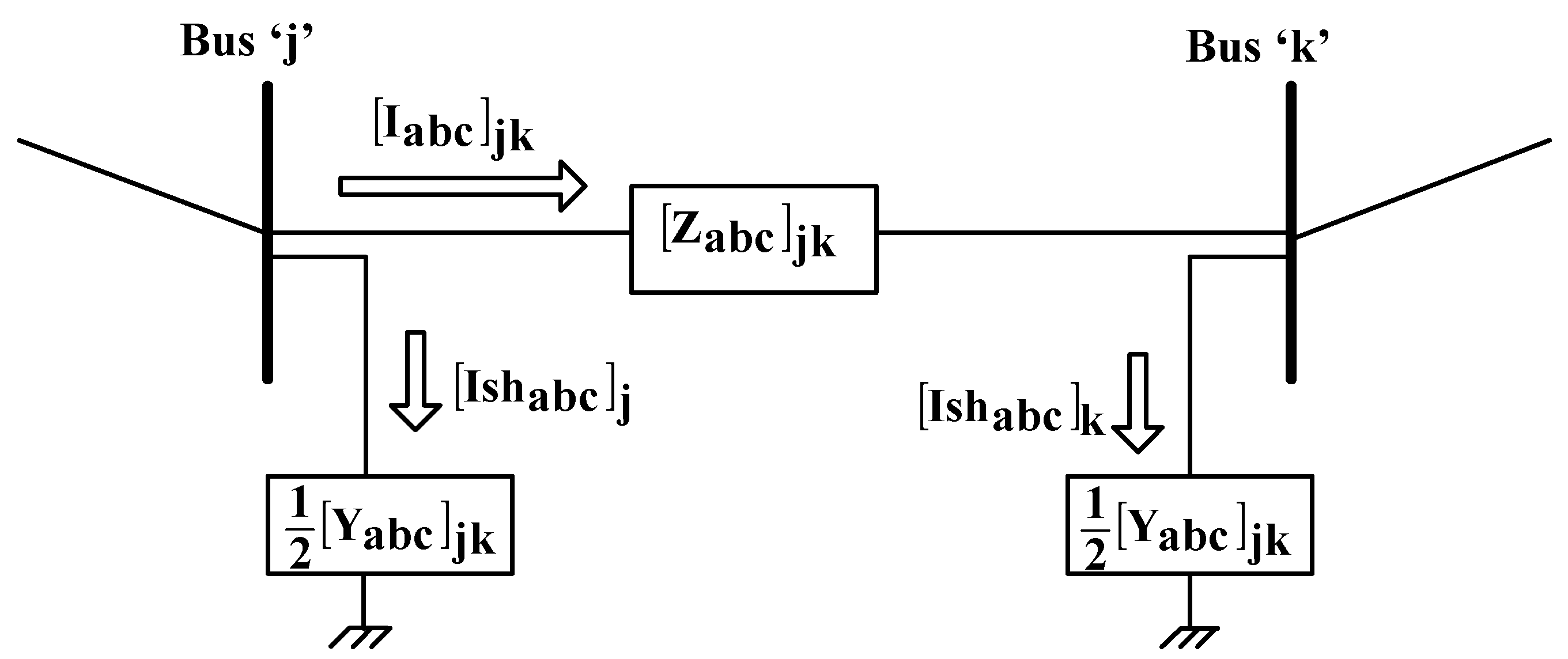
2.1. Modeling of Lines
2.2. Modeling of Loads
2.3. Modeling of Capacitor Banks
2.4. Modeling of Three-Phase Transformers
2.5. Renewable Energy Source
2.5.1. Synchronous Generator
2.5.2. Induction Generator
2.5.3. Power Electronic Converter
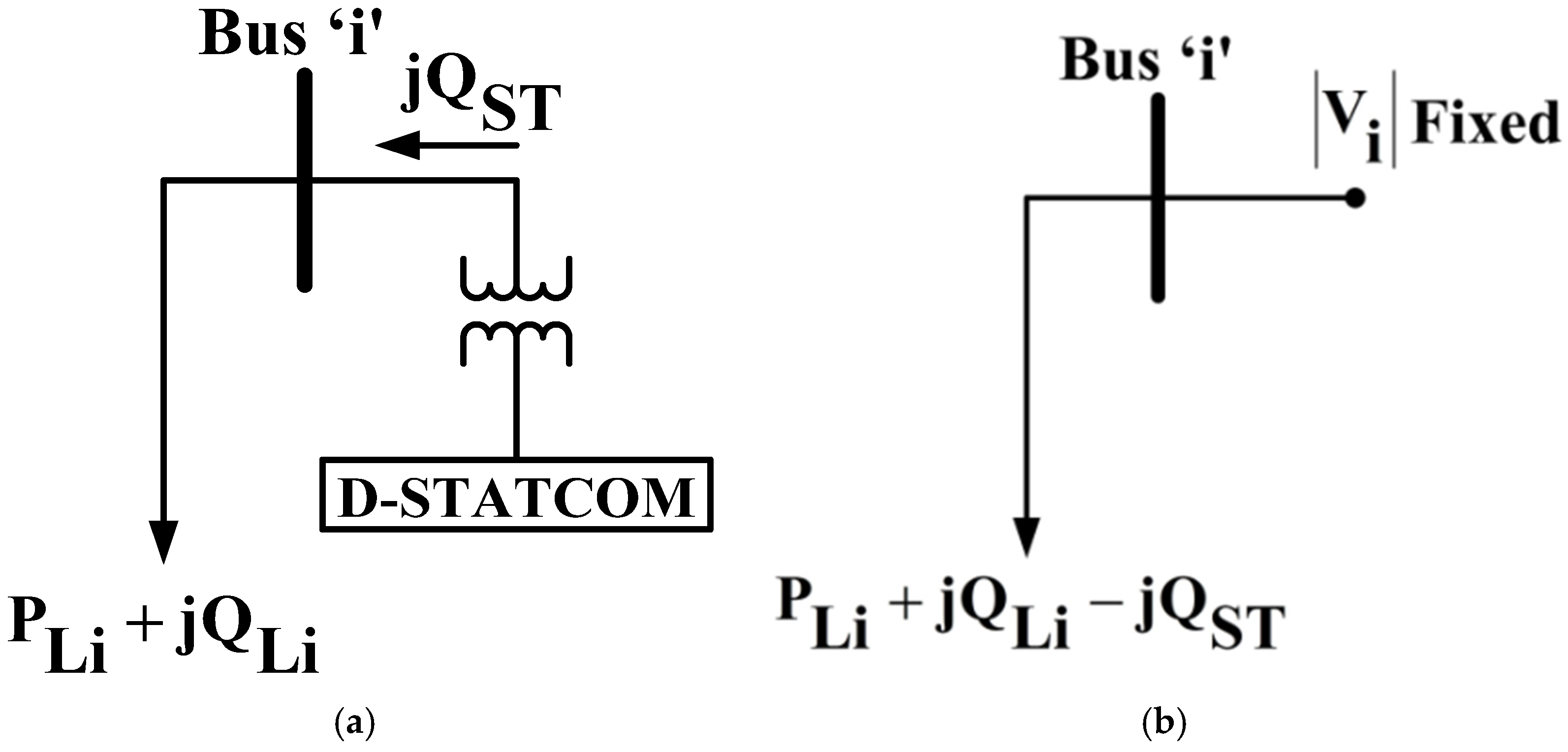
2.6. D-STATCOM
3. Voltage Unbalance
- V2: Negative sequence component of voltage;
- V1: Positive sequence component of voltage.
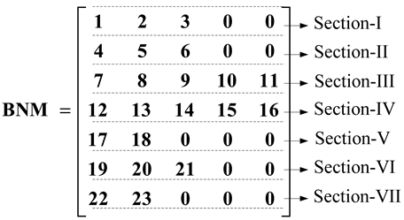
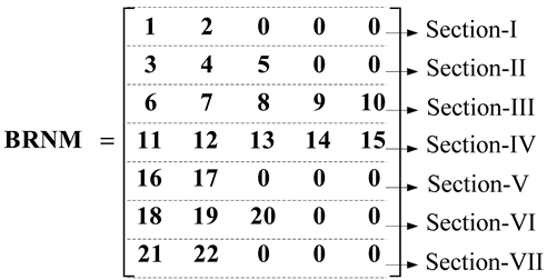
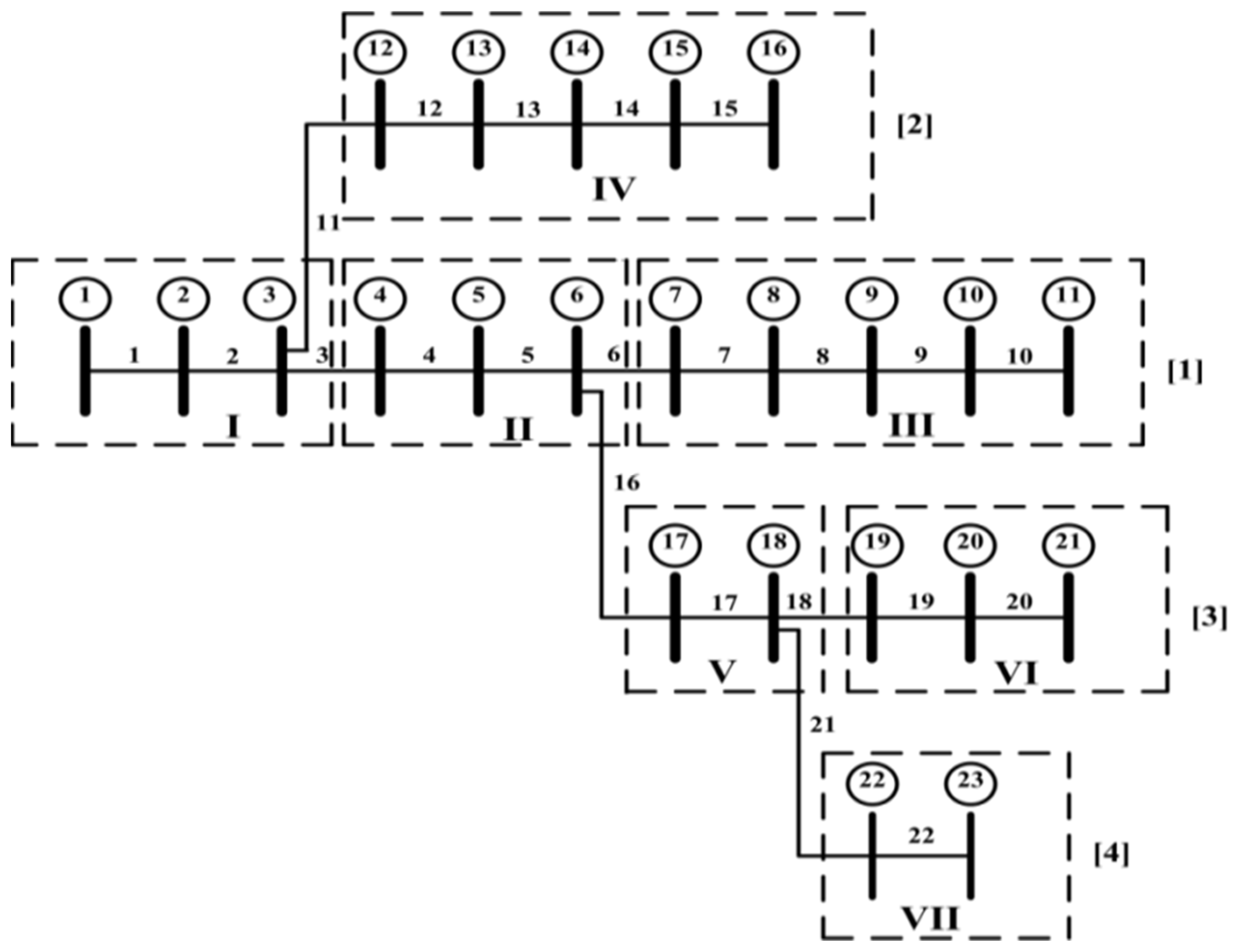
4. Algorithm for Developing the BNM and BRNM
- Starting with BN = 1, read the RE of the BN, i.e., 2. Then, check how many times this 2 appears in the SE row. From the above table it appeared once. That means bus 2 is the sending end for only one branch. Fill these RE 2 and BN 1 into two different variables (BNM and BRNM) as the first row and first column elements. Then, increase the column number by one.
- Increase the BN (i.e., BN = 2), read the RE of the BN, i.e., 3. Then, as in step 1, check for the appearance of 3 in the SE row. Bus 3 appeared twice. That means that two branches leave from bus 3. Then, fill these RE 3 and BN 2 into the same variables as the first row and present the column elements. Name this row’s elements as section-I. Now increase the row number by one and set the column number to one.
- Similarly, increase the BN, read the RE of the BN. Then, check for the appearance of this RE in the SE row. If it appears once, then fill these RE and BN values in as the present row and present column elements of variables BNM and BRNM. Then, increase the column number by one. Repeat step 4. If it does not appear or does appear more than one time in the SE row, then fill the corresponding RE and BN values as present row and present column elements. Then, identify this row as a section. Then, increase the row number by one and set the column number to one. Additionally, repeat step 4.
5. Three-Phase PFA with RESs and D-STATCOMs
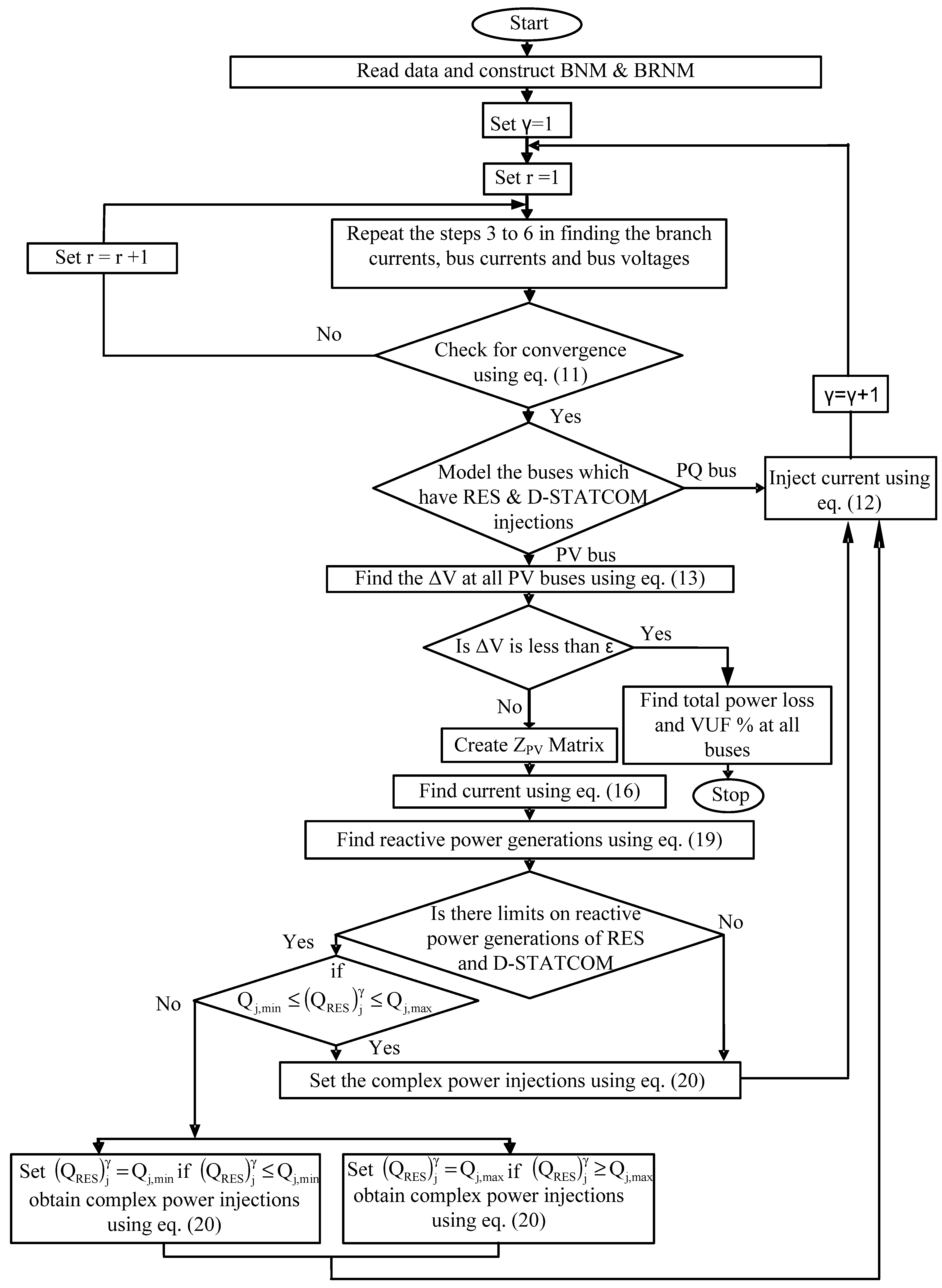
- Set iteration number γ = 1.
- Set iteration number r = 1.
- All bus voltages are allocated as the voltage at the sub-station bus.
- 4.
- Find the line current matrix serving the load at all buses.
- 5.
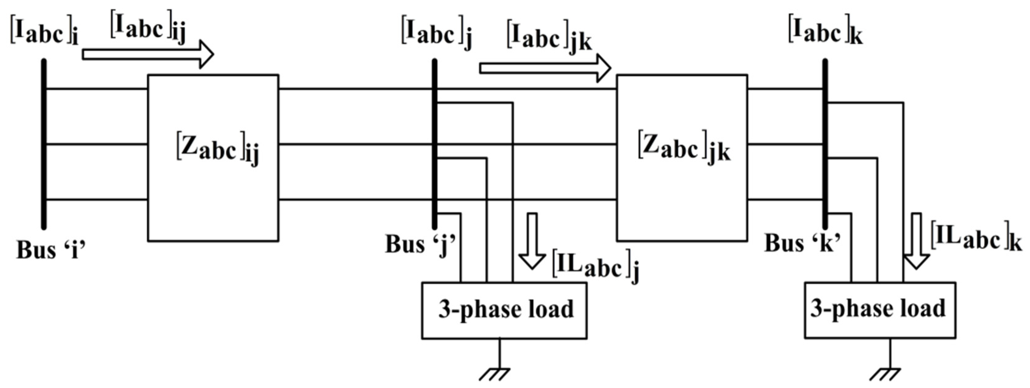
- Start with the collecting line current matrix at bus-23 (the tail bus in section-VII in the BNM) thereby find the line current matrix for branch-22 (the tail branch in section-VII in the BRNM). Then, continue to bus-22 and branch-21 to find the line current matrix at the bus and the line current matrix in the branch, respectively. From Figure 4, the following equations are obtained by applying KCL at every bus:where,: line current matrix at bus-k;: line current matrix for branch-jk;: line current matrix for load at bus-k;: line current matrix for shunt admittance at bus-k;: line current matrix for capacitor bank at bus-k, if any;: line current matrix injected by an RES or a D-STATCOM at busk, if any (for γ = 1, take this current injection as zero).
- 6.
- Now go to section-VI and repeat the procedure as in step 5 to find the line current matrix at the head bus and the line current matrix for the head branch. Similarly, proceed to upto section-I and find the line current matrix upto bus-1 and the line current matrix upto branch-1.
- 7.
- Now start with the head bus in section-I and continue to the tail bus in section-1 by finding the phase voltage matrix at all buses with Equation (1). Then, go to the next section and repeat the same procedure.
- 8.
- Steps 4 to 7 are to be repeated until the convergence criterion as given in Equation (11) is satisfied:
- 9.
- Locations of both the RES and D-STATCOM are to be selected.
- 10.
- Examine the RES type for the γ-th outside iteration.
- 11.
- If at the j-th bus the modeling of the RES is PQ, then the line current injection matrix at that bus is calculated with Equation (12):
- 12.
- If the modeling of the RES and D-STATCOM device at a bus is PV, then mismatches in voltages are calculated with Equation (13):
- 13.
- If Equation (14) is not satisfied at PV buses, then in order to maintain the specified voltages at these buses, the incremental current injection matrices are obtained with Equation (15):
- 14.
- If the RES and D-STATCOM device are able to generate unlimited Q, then the incremental reactive current injection matrix at the j-th PV bus is calculated with Equation (16):
- 15.
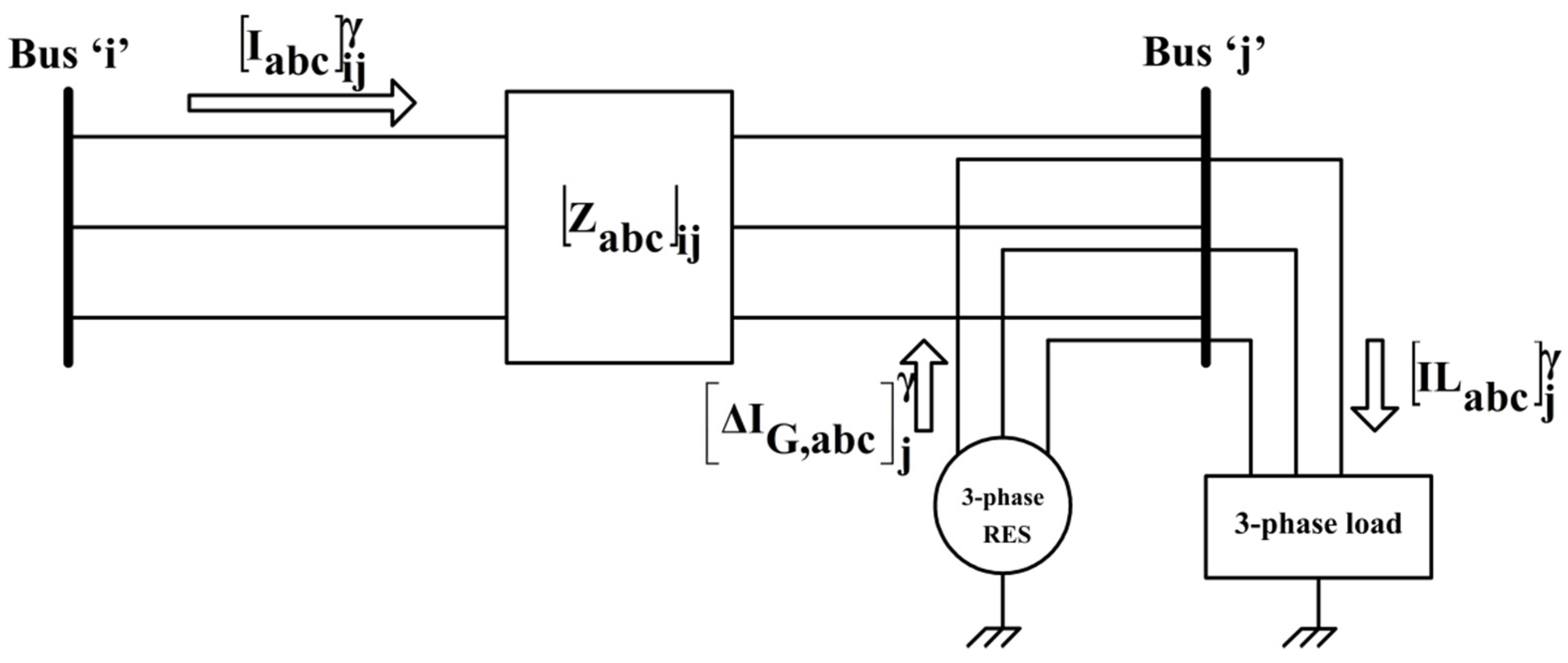
- As displayed in Figure 5, by applying KCL at the j-th bus, the line current matrix for branch ‘ij’ can be obtained with Equation (17):
- 16.
- The injected line current matrix at the RES and D-STATCOM device is obtained with Equation (12) by using the matrix for complex power generation given in Equation (20).
- 17.
- If the RES and D-STATCOM device are able to generate limited Q, then find the total Q generation of the RES and D-STATCOM device with Equation (21). The total Q generation of the RES and D-STATCOM device is now compared with the maximum and minimum limits of Q generation of the RES and D-STATCOM device, respectively. Limits:
- 18.
- Using the line current injection matrix at all PV buses, repeat from step 3 by setting γ = γ + 1.
- 19.
- Stop the iterative procedure when the convergence criteria is attained for every PV bus as given by Equation (14).
- 20.
- The complex power loss matrix for each branch is calculated with Equation (23).
- 21.
- Find the total power loss of the network and VUF% at each bus by using Equation (4).
6. Results and Discussions
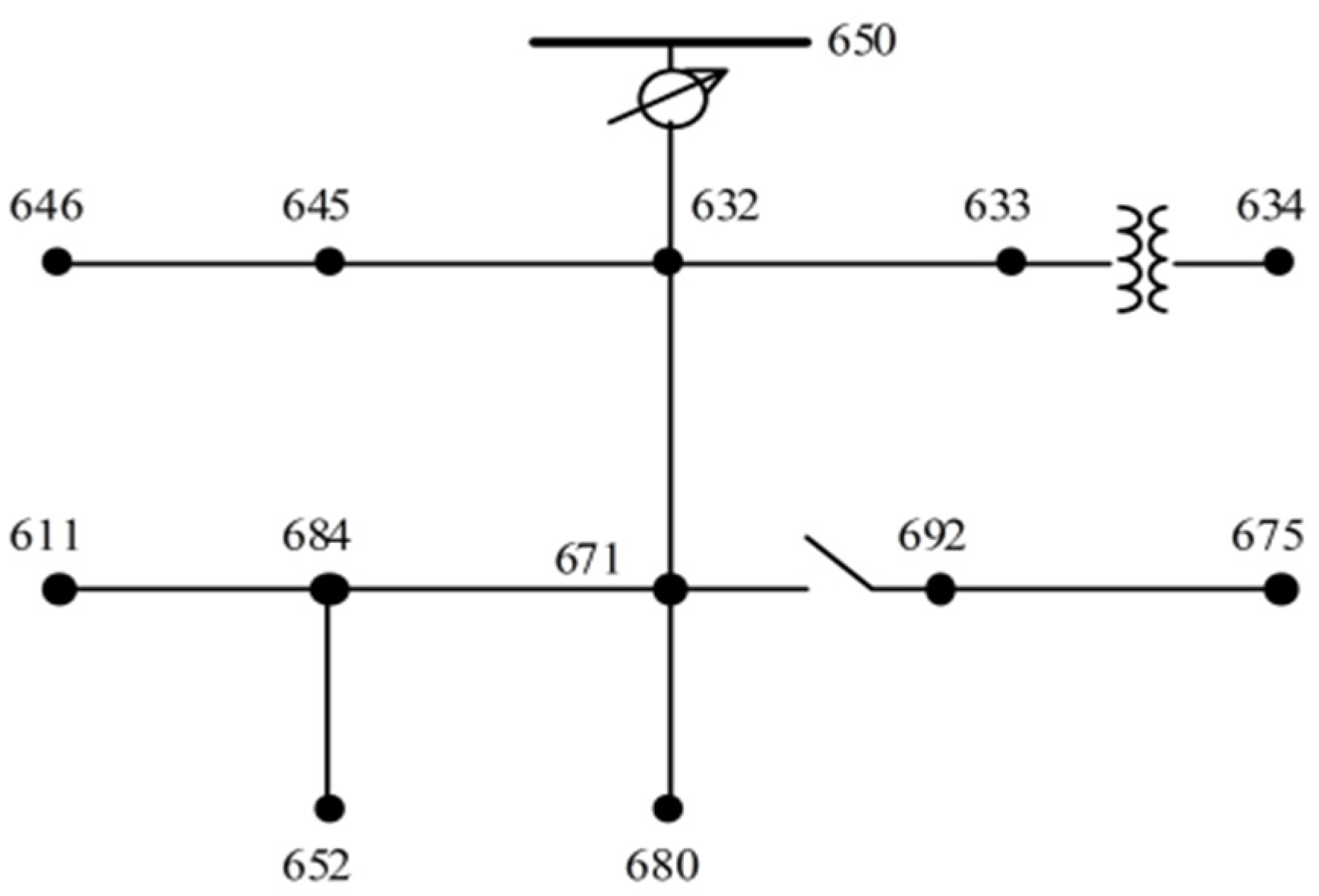
6.1. IEEE-13 Bus URDN
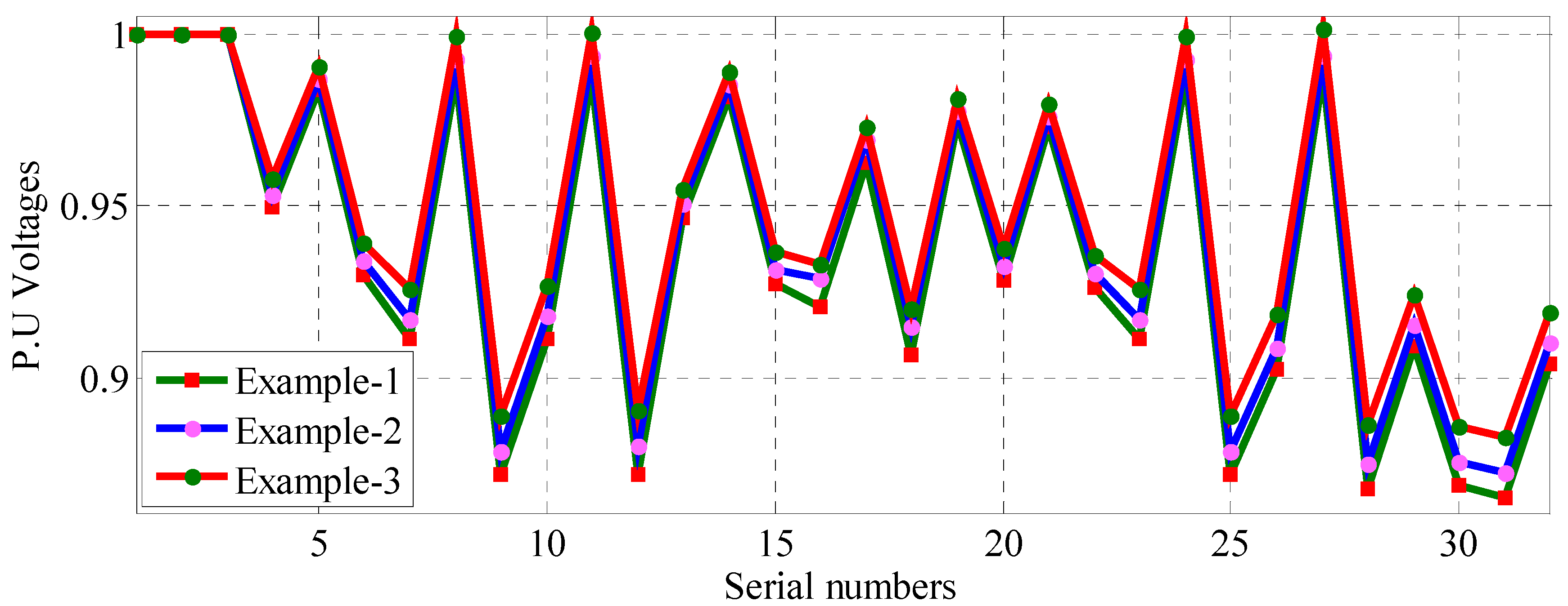
6.2. IEEE-13 Bus URDN with Study Examples
6.3. Discussion
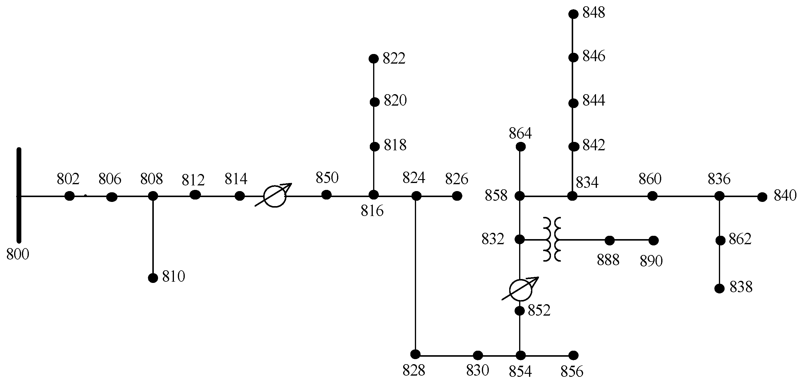
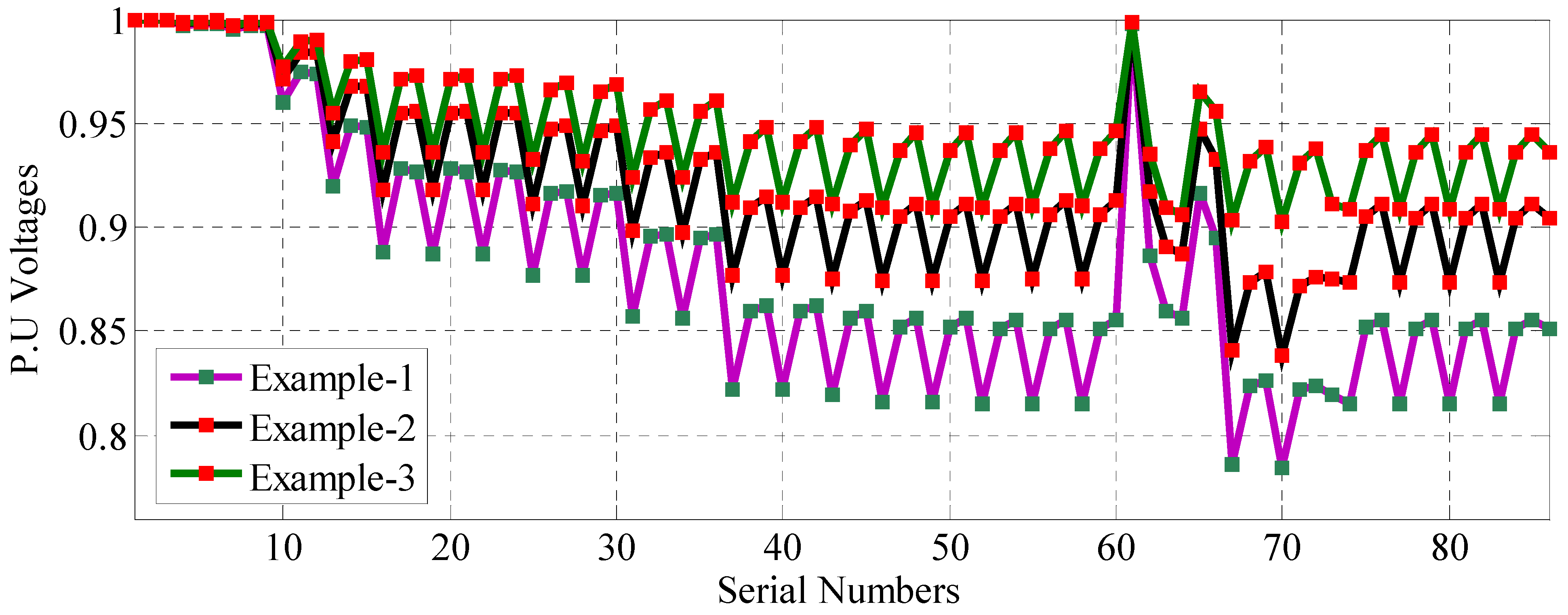
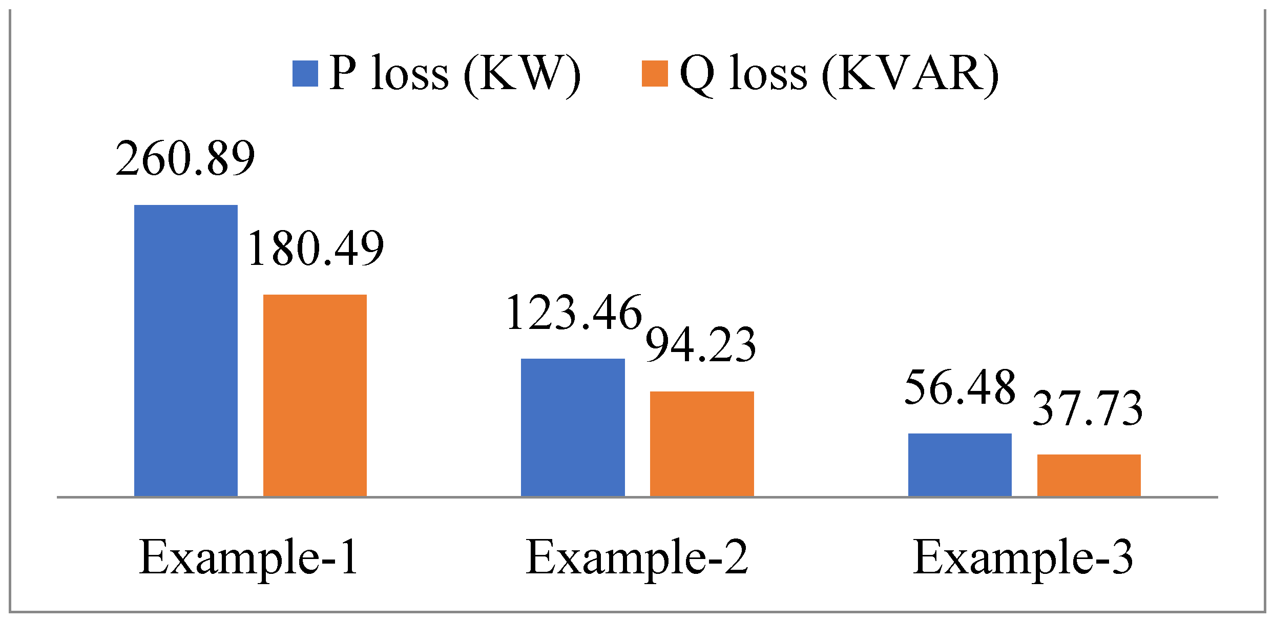
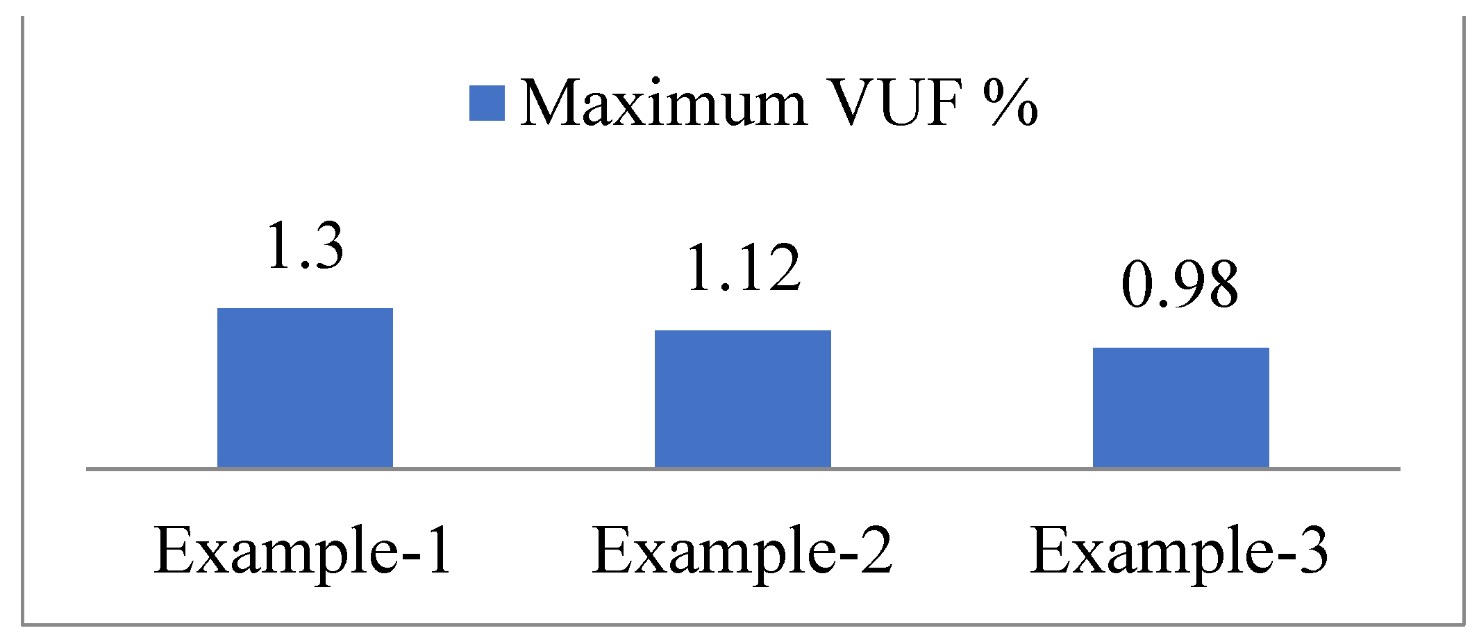
6.4. Study Examples and Discussion of the IEEE-34 Bus URDN
7. Conclusions
Author Contributions
Funding
Conflicts of Interest
References
- Rodríguez, F.J.R.; Hernandez, J.C.; Jurado, F. Voltage unbalance assessment in secondary radial distribution networks with single-phase photovoltaic systems. Int. J. Electr. Power Energy Syst. 2015, 64, 646–654. [Google Scholar] [CrossRef]
- Nour, A.M.; Helal, A.A.; El-Saadawi, M.M.; Hatata, A.Y. A control scheme for voltage unbalance mitigation in distribution network with rooftop PV systems based on distributed batteries. Int. J. Electr. Power Energy Syst. 2021, 124, 106375. [Google Scholar] [CrossRef]
- Abdoli, O.; Gholipour, E.; Hooshmand, R.-A. A New Approach to Compensating Voltage Unbalance by UPQC-Based PAC. Electr. Power Compon. Syst. 2018, 46, 1769–1781. [Google Scholar] [CrossRef]
- Girigoudar, K.; Roald, L.A. On the impact of different voltage unbalance metrics in distribution system optimization. Electr. Power Syst. Res. 2020, 189, 106656. [Google Scholar] [CrossRef]
- Cheng, C.S.; Shirmohammadi, D. A three-phase power flow method for real-time distribution system analysis. IEEE Trans. Power Syst. 1995, 10, 671–679. [Google Scholar] [CrossRef]
- Kumar, A.; Jha, B.K.; Singh, D.; Misra, R.K. A New Current Injection Based Power Flow Formulation. Electr. Power Compon. Syst. 2020, 48, 268–280. [Google Scholar] [CrossRef]
- IEEE. IEEE Standard for Interconnecting Distributed Resources with Electric Power Systems; IEEE: Piscataway, NJ, USA, 2003; pp. 1–28. [Google Scholar] [CrossRef]
- Abdelaziz, A.Y.; Hegazy, Y.G.; El-Khattam, W.; Othman, M.M. A Multi-objective Optimization for Sizing and Placement of Voltage-controlled Distributed Generation Using Supervised Big Bang–Big Crunch Method. Electr. Power Compon. Syst. 2015, 43, 105–117. [Google Scholar] [CrossRef]
- Othman, M.M.; Hegazy, Y.; Abdelaziz, A. Electrical energy management in unbalanced distribution networks using virtual power plant concept. Electr. Power Syst. Res. 2017, 145, 157–165. [Google Scholar] [CrossRef]
- Abdelaziz, A.Y.; Hegazy, Y.G.; El-Khattam, W.; Othman, M.M. Optimal Planning of Distributed Generators in Distribution Networks Using Modified Firefly Method. Electr. Power Compon. Syst. 2015, 43, 320–333. [Google Scholar] [CrossRef]
- Abdelaziz, A.; Hegazy, Y.; El-Khattam, W.; Othman, M. Optimal allocation of stochastically dependent renewable energy based distributed generators in unbalanced distribution networks. Electr. Power Syst. Res. 2015, 119, 34–44. [Google Scholar] [CrossRef]
- Tolba, M.A.; Rezk, H.; Tulsky, V.; Diab, A.A.Z.; Abdelaziz, A.Y.; Vanin, A. Impact of Optimum Allocation of Renewable Distributed Generations on Distribution Networks Based on Different Optimization Algorithms. Energies 2018, 11, 245. [Google Scholar] [CrossRef] [Green Version]
- Serem, N.; Letting, L.; Munda, J. Voltage Profile and Sensitivity Analysis for a Grid Connected Solar, Wind and Small Hydro Hybrid System. Energies 2021, 14, 3555. [Google Scholar] [CrossRef]
- Zarco-Soto, F.; Zarco-Periñán, P.; Martínez-Ramos, J. Centralized Control of Distribution Networks with High Penetration of Renewable Energies. Energies 2021, 14, 4283. [Google Scholar] [CrossRef]
- Gotham, D.J.; Heydt, G.T. Power flow control and power flow studies for systems with FACTS devices. IEEE Trans. Power Syst. 1998, 13, 60–65. [Google Scholar] [CrossRef]
- Yang, Z.; Shen, C.; Crow, M.L.; Zhang, L. An improved STATCOM model for power flow analysis. In Proceedings of the Power Engineering Society Summer Meeting, Seattle, WA, USA, 16–20 July 2000; Volume 2, pp. 1121–1126. [Google Scholar] [CrossRef]
- Jazebi, S.; Hosseinian, S.; Vahidi, B. DSTATCOM allocation in distribution networks considering reconfiguration using differential evolution algorithm. Energy Convers. Manag. 2011, 52, 2777–2783. [Google Scholar] [CrossRef]
- Rezaeian-Marjani, S.; Galvani, S.; Talavat, V.; Farhadi-Kangarlu, M. Optimal allocation of D-STATCOM in distribution networks including correlated renewable energy sources. Int. J. Electr. Power Energy Syst. 2020, 122, 106178. [Google Scholar] [CrossRef]
- Patel, S.K.; Arya, S.R.; Maurya, R. Optimal Step LMS-Based Control Algorithm for DSTATCOM in Distribution System. Electr. Power Compon. Syst. 2019, 47, 675–691. [Google Scholar] [CrossRef]
- Sirjani, R.; Jordehi, A.R. Optimal placement and sizing of distribution static compensator (D-STATCOM) in electric distribution networks: A review. Renew. Sustain. Energy Rev. 2017, 77, 688–694. [Google Scholar] [CrossRef]
- Sayahi, K.; Kadri, A.; Bacha, F.; Marzougui, H. Implementation of a D-STATCOM control strategy based on direct power control method for grid connected wind turbine. Int. J. Electr. Power Energy Syst. 2020, 121, 106105. [Google Scholar] [CrossRef]
- Relić, F.; Marić, P.; Glavaš, H.; Petrović, I. Influence of FACTS Device Implementation on Performance of Distribution Network with Integrated Renewable Energy Sources. Energies 2020, 13, 5516. [Google Scholar] [CrossRef]
- Satish, R.; Kantarao, P.; Vaisakh, K. A new algorithm for impacts of multiple DGs and D-STATCOM in unbalanced radial distribution networks. Int. J. Renew. Energy Technol. 2021, 12, 221. [Google Scholar] [CrossRef]
- Kersting, W.H. Distribution System Modeling and Analysis, 4th ed.; CRC Press: Boca Raton, FL, USA, 2017. [Google Scholar]
- Khushalani, S. Unbalanced distribution power flow with distributed generation. In Proceedings of the IEEE/PES Transactions on Distribution Conference, Dallas, TX, USA, 21–24 May 2006; pp. 301–306. [Google Scholar] [CrossRef]
- Chen, T.-H.; Chen, M.-S.; Inoue, T.; Kotas, P.; Chebli, E. Three-phase cogenerator and transformer models for distribution system analysis. IEEE Trans. Power Deliv. 1991, 6, 1671–1681. [Google Scholar] [CrossRef]
- Losi, A.; Russo, M. Dispersed Generation Modeling for Object-Oriented Distribution Load Flow. IEEE Trans. Power Deliv. 2005, 20, 1532–1540. [Google Scholar] [CrossRef]
- Chen, H.; Chen, J.; Shi, D.; Duan, X. Power flow study and voltage stability analysis for distribution systems with distributed generation. In Proceedings of the IEEE Power Engineering Society General Meeting, Montreal, QC, Canada, 18–22 June 2006; pp. 1–8. [Google Scholar] [CrossRef]
- Naka, S.; Genji, T.; Fukuyama, Y. Practical equipment models for fast distribution power flow considering interconnection of distributed generators. In Proceedings of the Power Engineering Society Summer Meeting Conference Proceedings, Vancouver, BC, Canada, 15–19 July 2001; pp. 1007–1012. [Google Scholar] [CrossRef]
- Nehrir, H.; Wang, C.; Shaw, S. Fuel cells: Promising devices for distributed generation. IEEE Power Energy Mag. 2006, 4, 47–53. [Google Scholar] [CrossRef]
- Shahnia, F.; Majumder, R.; Ghosh, A.; Ledwich, G.; Zare, F. Voltage imbalance analysis in residential low voltage distribution networks with rooftop PVs. Electr. Power Syst. Res. 2011, 81, 1805–1814. [Google Scholar] [CrossRef]
- Singh, A.K.; Singh, G.K.; Mitra, R. Some Observations on Definitions of Voltage Unbalance. In Proceedings of the 39th North American Power Symposium (NAPS), Las Cruces, NM, USA, 30 September–2 October 2007; pp. 473–479. [Google Scholar] [CrossRef]
- Das, D.; Nagi, H.; Kothari, D. Novel method for solving radial distribution networks. IEE Proc.-Gener. Transm. Distrib. 1994, 141, 291–298. [Google Scholar] [CrossRef]
- Radial Distribution Test Feeders. Available online: http://sites.ieee.org/pes-testfeeders/resources (accessed on 2 August 2021).


| Wye Connected | Delta Connected | |
|---|---|---|
| Specified phase voltage matrix at a bus and reactive power matrix | , | , |
| Phase current matrix serving the capacitor bank | ||
| Line current matrix serving the capacitor bank |
| RES Type | Electric Machine | Utility Interface | Suitable Model for PFAs | Explanations |
|---|---|---|---|---|
| Fuel cell | Inverter | PV bus | CCC is intended to independently control P and V | |
| PQ bus | CCC is intended to independently control P and Q | |||
| Solar | Inverter | PV bus | CCC is intended to independently control P and V | |
| PQ bus | CCC is intended to independently control P and Q | |||
| Wind | FSIG | Directly | PQ bus | - |
| SVCM | ||||
| DFIG | Rectifier + Inverter | PV bus | CCC is intended to independently control P and V | |
| PQ bus | CCC is intended to independently control P and Q | |||
| Conventional or permanent magnet SG | Rectifier + Inverter | PV bus | CCC is intended to independently control P and V | |
| PQ bus | CCC is intended to independently control P and Q | |||
| Hydro | SG | Directly | PV bus | VEV in FTV |
| PQ bus | VEV in FPF | |||
| SVCM | CEV | |||
| Geothermal | SG | Directly | PV bus | VEV in FTV |
| PQ bus | VEV in FPF | |||
| SVCM | CEV | |||
| Biofuel | SG | Directly | PV bus | VEV in FTV |
| PQ bus | VEV in FPF | |||
| SVCM | CEV |
| Branch Number (BN) | Sending Bus (SE) | Receiving Bus (RE) |
|---|---|---|
| 1 | 1 | 2 |
| 2 | 2 | 3 |
| 3 | 3 | 4 |
| 4 | 4 | 5 |
| 5 | 5 | 6 |
| 6 | 6 | 7 |
| 7 | 7 | 8 |
| 8 | 8 | 9 |
| 9 | 9 | 10 |
| 10 | 10 | 11 |
| 11 | 3 | 12 |
| 12 | 12 | 13 |
| 13 | 13 | 14 |
| 14 | 14 | 15 |
| 15 | 15 | 16 |
| 16 | 6 | 17 |
| 17 | 17 | 18 |
| 18 | 18 | 19 |
| 19 | 19 | 20 |
| 20 | 20 | 21 |
| 21 | 18 | 22 |
| 22 | 22 | 23 |
| Phase | Obtained Power Loss | IEEE Losses [34] | ||
|---|---|---|---|---|
| P Loss (kW) | Q Loss (kVAR) | P Loss (kW) | Q Loss (kVAR) | |
| a | 39.13 | 152.62 | 39.18 | 152.59 |
| b | −4.74 | 42.27 | −4.70 | 42.22 |
| c | 76.59 | 129.69 | 76.65 | 129.85 |
| Total | 110.98 | 324.57 | 111.13 | 324.66 |
| Bus | Phase | Obtained Voltage Solution | IEEE Solution [34] | Error in Voltage Mag. | Error in Voltage Ang. |
|---|---|---|---|---|---|
| 650 | a | 1<0° | 1<0° | 0.0000 | 0.00 |
| b | 1<−120° | 1<−120° | 0.0000 | 0.00 | |
| c | 1<120° | 1<120° | 0.0000 | 0.00 | |
| RG | a | 1.0625<0° | 1.0625<0° | 0.0000 | 0.00 |
| b | 1.0500<−120° | 1.0500<−120° | 0.0000 | 0.00 | |
| c | 1.0687<120° | 1.0687<120° | 0.0000 | 0.00 | |
| 632 | a | 1.0210<−2.49° | 1.0210<−2.49° | 0.0000 | 0.00 |
| b | 1.0420<−121.72° | 1.0420<−121.72° | 0.0000 | 0.00 | |
| c | 1.0175<117.83° | 1.0170<117.83° | −0.0005 | 0.00 | |
| 671 | a | 0.9900<−5.30° | 0.9900<−5.30° | 0.0000 | 0.00 |
| b | 1.0529<−122.34° | 1.0529<−122.34° | 0.0000 | 0.00 | |
| c | 0.9778<116.03° | 0.977<116.02° | 0.0001 | −0.01 | |
| 680 | a | 0.9900<−5.30° | 0.9900<−5.30° | 0.0000 | 0.00 |
| b | 1.0529<−122.34° | 1.0529<−122.34° | 0.0000 | 0.00 | |
| c | 0.9778<116.03° | 0.977<116.02° | 0.0001 | −0.01 | |
| 633 | a | 1.0180<−2.55° | 1.0180<−2.56° | 0.0000 | 0.01 |
| b | 1.0401<−121.77° | 1.0401<−121.77° | 0.0000 | 0.00 | |
| c | 1.0148<117.82° | 1.0148<117.82° | 0.0000 | 0.00 | |
| 634 | a | 0.9940<−3.23° | 0.9940<−3.23° | 0.0000 | 0.00 |
| b | 1.0218<−122.22° | 1.0218<−122.22° | 0.0000 | 0.00 | |
| c | 0.9960<117.35° | 0.9960<117.34° | 0.0000 | −0.01 | |
| 645 | b | 1.0328<−121.90° | 1.0329<−121.90° | 0.0001 | 0.00 |
| c | 1.0155<117.86° | 1.0155<117.86° | 0.0001 | 0.00 | |
| 646 | b | 1.0311<−121.98° | 1.0311<−121.98° | 0.0000 | 0.00 |
| c | 1.0134<117.90° | 1.0134<117.90° | 0.0000 | 0.01 | |
| 692 | a | 0.9900<−5.30° | 0.9900<−5.31° | 0.0000 | 0.01 |
| b | 1.0529<−122.34° | 1.0529<−122.34° | 0.0000 | 0.00 | |
| c | 0.9778<116.03° | 0.9777<116.02° | −0.0001 | −0.01 | |
| 675 | a | 0.9835<−5.55° | 0.9835<−5.56° | 0.0000 | 0.01 |
| b | 1.0553<−122.52° | 1.0553<−122.52° | 0.0000 | 0.00 | |
| c | 0.9759<116.04° | 0.9758<116.03° | −0.0001 | −0.01 | |
| 684 | a | 0.9881<−5.32° | 0.9881<−5.32° | 0.0000 | 0.00 |
| c | 0.9758<115.92° | 0.9758<115.92° | 0.0000 | 0.00 | |
| 611 | c | 0.9738<115.78° | 0.9738<115.78° | 0.0000 | 0.00 |
| 652 | a | 0.9825<−5.24° | 0.9825<−5.25° | 0.0000 | 0.01 |
| Study Examples | Specification | |||
|---|---|---|---|---|
| Example1 | • Voltage regulator is taken off between bus-650 and bus-632 • Capacitor banks are taken off at bus-675 and bus-611 | |||
| Device | Location | Modeling | Rating [23] | |
| Example2 | Three-phase RES | Bus-634 | PQ | P = 300 kW/phase and Q = 197 kVAR/phase |
| Three-phase RES | Bus-675 | PV | P = 260 kW/phase and 3-phase Q limits: 100 ≤ Q ≤ 650 kVAR | |
| Example3 | Three-phase RES | Bus-634 | PQ | P = 300 kW/phase and Q = 197 kVAR/phase |
| Three-phase RES | Bus-675 | PV | P = 260 kW/phase and 3-phase Q limits: 100 ≤ Q ≤ 650 kVAR | |
| Three-phase D-STATCOM | Bus-680 | PV | P = 0 and 3-phase Q limits: 100 ≤ Q ≤ 500 kVAR | |
| Phase | Example-1 | Example-2 | Example-3 | |||
|---|---|---|---|---|---|---|
| P Loss (kW) | Q Loss (kVAR) | P Loss (kW) | Q Loss (kVAR) | P Loss (kW) | Q Loss (kVAR) | |
| A | 39.48 | 194.82 | 7.9867 | 87.6800 | 7.9589 | 83.4026 |
| B | −2.03 | 47.13 | 4.0219 | 10.1590 | 2.9510 | 9.6542 |
| C | 109.88 | 191.59 | 56.8390 | 88.4051 | 53.9973 | 81.2180 |
| Total | 147.33 | 433.54 | 68.84 | 186.24 | 64.90 | 174.27 |
| Bus | S. No | Ph | Example1 | Example2 | Example3 | |||
|---|---|---|---|---|---|---|---|---|
| VUF% | VUF% | VUF% | ||||||
| 650 | 1 | a | 1<0° | 0 | 1.0000<0° | 0 | 1.0000<0° | 0 |
| 2 | b | 1<−120° | 1.0000<−120° | 1.0000<−120° | ||||
| 3 | c | 1<120° | 1.0000<120° | 1.0000<120° | ||||
| 632 | 4 | a | 0.9498<−2.74° | 1.27 | 0.9730<−1.68° | 0.83 | 0.9752<−1.73° | 0.81 |
| 5 | b | 0.9839<−121.68° | 0.9973<−120.48° | 0.9994<−120.49° | ||||
| 6 | c | 0.9300<117.80° | 0.9540<118.98° | 0.9566<118.92° | ||||
| 671 | 7 | a | 0.9109<−5.89° | 2.58 | 0.9429<−4.10° | 1.89 | 0.9474<−4.19° | 1.88 |
| 8 | b | 0.9875<−122.20° | 1.0045<−120.42° | 1.0088<−120.44° | ||||
| 9 | c | 0.8717<115.95° | 0.9056<117.88° | 0.9109<117.77° | ||||
| 680 | 10 | a | 0.9109<−5.89° | 2.58 | 0.9429<−4.10° | 1.89 | 0.9485<−4.22° | 1.88 |
| 11 | b | 0.9875<−122.20° | 1.0045<−120.42° | 1.0099<−120.45° | ||||
| 12 | c | 0.8717<115.95° | 0.9056<117.87° | 0.9121<117.74° | ||||
| 633 | 13 | a | 0.9466<−2.82° | 1.28 | 0.9749<−1.64° | 0.82 | 0.9772<−1.69° | 0.81 |
| 14 | b | 0.9819<−121.73° | 1.0006<−120.40° | 1.0027<−120.42° | ||||
| 15 | c | 0.9271<117.79° | 0.9574<119.06° | 0.9600<119.01° | ||||
| 634 | 16 | a | 0.9207<−3.60° | 1.35 | 0.9950<−1.00° | 0.76 | 0.9972<−1.05° | 0.76 |
| 17 | b | 0.9624<−122.24° | 1.0249<−119.60° | 1.0270<−119.62° | ||||
| 18 | c | 0.9064<117.21° | 0.9828<119.94° | 0.9853<119.88° | ||||
| 645 | 19 | b | 0.9745<−121.86° | 0.9880<−120.66° | 0.9901<−120.67° | |||
| 20 | c | 0.9283<117.82° | 0.9523<119.00° | 0.9549<118.95° | ||||
| 646 | 21 | b | 0.9729<−121.93° | 0.9863<−120.73° | 0.9884<−120.75° | |||
| 22 | c | 0.9264<117.86° | 0.9503<119.05° | 0.9529<118.99° | ||||
| 692 | 23 | a | 0.9109<−5.89° | 2.58 | 0.9429<−4.10° | 1.89 | 0.9474<−4.19° | 1.88 |
| 24 | b | 0.9875<−122.20° | 1.0045<−120.42° | 1.0088<−120.44° | ||||
| 25 | c | 0.8717<115.95° | 0.9056<117.87° | 0.9109<117.77° | ||||
| 675 | 26 | a | 0.9025<−6.07° | 2.75 | 0.9379<−4.19° | 2.00 | 0.9424<−4.28° | 1.99 |
| 27 | b | 0.9887<−122.30° | 1.0080<−120.44° | 1.0123<−120.47° | ||||
| 28 | c | 0.8678<116.06° | 0.9047<118.08° | 0.9099<117.97° | ||||
| 684 | 29 | a | 0.9093<−5.95° | 0.9411<−4.15° | 0.9456<−4.24° | |||
| 30 | c | 0.8684<115.91° | 0.9023<117.84° | 0.9076<117.74° | ||||
| 611 | 31 | c | 0.8651<115.83° | 0.8990<117.77° | 0.9043<117.66° | |||
| 652 | 32 | a | 0.9041<−5.87° | 0.9358<−4.07° | 0.9403<−4.17° | |||
| Study Examples | Specification | |||
|---|---|---|---|---|
| Example1 | • Voltage regulator is taken off between bus-614 and bus-650 and bus-852–bus-832. • Capacitor banks are taken off at bus-844 and bus-848. | |||
| Device | Location | Modeling | Rating | |
| Example2 | Three-phase RES | Bus-848 | PQ | P = 150 kW/phase and Q = 99 kVAR/phase |
| Three-phase D-STATCOM | Bus-650 | PV | P = 0 and 3-phase Q limits: 50 ≤ Q ≤ 250 kVAR. | |
| Example3 | Three-phase RES | Bus-848 | PQ | P = 150 kW/phase and Q = 99 kVAR/phase |
| Three-phase RES | Bus-890 | PV | P = 130 kW/phase and 3-phase Q limits: 50 ≤ Q ≤ 325 kVAR. | |
| Three-phase D-STATCOM | Bus-650 | PV | P = 0 and 3-phase Q limits: 50 ≤ Q ≤ 250 kVAR. | |
Publisher’s Note: MDPI stays neutral with regard to jurisdictional claims in published maps and institutional affiliations. |
© 2021 by the authors. Licensee MDPI, Basel, Switzerland. This article is an open access article distributed under the terms and conditions of the Creative Commons Attribution (CC BY) license (https://creativecommons.org/licenses/by/4.0/).
Share and Cite
Satish, R.; Vaisakh, K.; Abdelaziz, A.Y.; El-Shahat, A. A Novel Three-Phase Power Flow Algorithm for the Evaluation of the Impact of Renewable Energy Sources and D-STATCOM Devices on Unbalanced Radial Distribution Networks. Energies 2021, 14, 6152. https://doi.org/10.3390/en14196152
Satish R, Vaisakh K, Abdelaziz AY, El-Shahat A. A Novel Three-Phase Power Flow Algorithm for the Evaluation of the Impact of Renewable Energy Sources and D-STATCOM Devices on Unbalanced Radial Distribution Networks. Energies. 2021; 14(19):6152. https://doi.org/10.3390/en14196152
Chicago/Turabian StyleSatish, Raavi, Kanchapogu Vaisakh, Almoataz Y. Abdelaziz, and Adel El-Shahat. 2021. "A Novel Three-Phase Power Flow Algorithm for the Evaluation of the Impact of Renewable Energy Sources and D-STATCOM Devices on Unbalanced Radial Distribution Networks" Energies 14, no. 19: 6152. https://doi.org/10.3390/en14196152