Article

Impacts of Extreme Ambient Temperatures and Road Gradient on Energy Consumption and CO2 Emissions of a Euro 6d-Temp Gasoline Vehicle

by
Barouch Giechaskiel
*,
Dimitrios Komnos
and
Georgios Fontaras
*
Joint Research Centre (JRC), European Commission, Via E. Fermi 2749, 21027 Ispra, Italy
*
Authors to whom correspondence should be addressed.
Energies 2021, 14(19), 6195; https://doi.org/10.3390/en14196195
Submission received: 4 September 2021 / Revised: 22 September 2021 / Accepted: 24 September 2021 / Published: 28 September 2021

Abstract

:
The EU aims to substantially reduce its greenhouse gas emissions in the following decades and achieve climate neutrality by 2050. Better CO2 estimates, particularly in urban conditions, are necessary for assessing the effectiveness of various regional policy strategies. In this study, we measured the CO2 emissions of a Euro 6d-temp gasoline direct injection (GDI) vehicle with a three-way catalyst (TWC) and a gasoline particulate filter (GPF) at ambient temperatures from −30 °C up to 50 °C with the air-conditioning on. The tests took place both on the road and in the laboratory, over cycles simulating congested urban traffic, dynamic driving, and uphill driving towing a trailer at 85% of the maximum payloads of both the car and the trailer. The CO2 values varied over a wide range depending on the temperature and driving conditions. Vehicle simulation was used to quantify the effect of ambient temperature, vehicle weight and road grade on the CO2 emissions. The results showed that vehicle energy demand was significantly increased under the test conditions. In urban trips, compared to the baseline at 23 °C, the CO2 emissions were 9–20% higher at −10 °C, 30–44% higher at −30 °C, and 37–43% higher at 50 °C. Uphill driving with a trailer had 2–3 times higher CO2 emissions. In motorway trips at 50 °C, CO2 emissions increased by 13–19%. The results of this study can help in better quantification of CO2 and fuel consumption under extreme conditions. Additional analysis on the occurrence of such conditions in real-world operation is advisable.

1. Introduction

The European Union (EU) has set targets to become carbon neutral by 2050 progressively. Interestingly, studies have suggested that low-carbon energy policies may improve air pollution [1,2]. The transport sector, in which road transport is the biggest contributor of greenhouse gas emissions, is the only sector of the economy that has not achieved emissions reductions in the past decades [3]. Vehicle energy consumption and the resulting CO2 or other greenhouse gas emissions are at the core of policy initiatives worldwide, as increasingly more countries commit to addressing global warming. In the EU, Regulation (EU) 2019/631/EC mandates, in addition to certification-based CO2 targets, the monitoring of CO2 emissions and energy consumption over real-world vehicle operation. This provision came as a response to previous evidence suggesting that the improvements in fuel consumption and carbon emissions of road vehicles, observed on official certification data, were not fully reflected in actual operation [4,5]. Recent estimates [6] suggest that moving to a new test procedure [7,8] has helped contain the problem at the EU level; however, the differences are still high. EU regulation requires active monitoring of the difference between official and actual emissions at the fleet level. For this purpose, new vehicles sold in the EU are equipped with on-board fuel consumption monitoring systems [9], and new regulations are being implemented for communicating these values periodically, aiming to achieve maximum fleet coverage [10].
Contrary to laboratory test conditions, real-world driving exposes vehicles to extreme operating conditions such as very high or very low temperatures, intense road gradients, extreme congestion, or payload conditions outside the regular certification boundaries. Such factors need to be considered when analysing the nature and origins of the difference between laboratory real-world fuel consumption. In addition, it is crucial to address both vehicle CO2 emissions and the energy needed to propel the vehicles. This last aspect becomes evident when considering the most prominent technologies for transport decarbonization, i.e., electrified vehicles, such as battery electric vehicles, plug-in hybrids, or fuel cell vehicles. Energy consumption directly impacts well-to-tank emissions and vehicle range. The first may result in high CO2 emissions in countries where primary energy is produced from carbon-intensive fossil fuels [11,12]. Range reductions may hamper the technology uptake as long as the refuelling network remains undeveloped [13].
Driving style, trip duration and distance, ambient conditions, road morphology, and traffic all affect the energy consumption of a vehicle and its CO2 emissions and range [14,15,16,17]. A detailed study demonstrated the impact of different factors on the pollutant and CO2 emissions of conventional light and heavy-duty vehicles [18]. In certain cases, electrified vehicles may even suffer more from extreme operating conditions, resulting in increased CO2 emissions if the electricity used for battery charging originates from the combustion of fossil fuels. A study found a 50% reduction at −20 °C and 30% reduction at 40 °C ambient temperature [19]. For similar variation temperature ranges, the impact on CO2 emissions of a conventional vehicle was reported to be much lower, ranging between 4 and 15% [14]. Similarly, road gradient may significantly contribute to the energy consumption, particularly when combined with congested or dynamic drive conditions [20] where the potential energy stored in the vehicle during uphill driving cannot be extensively recuperated during downhill driving. Several recent studies focus on factors such as ambient wind [21], road grade [22,23,24], or combinations thereof [25,26]. The studies of effect of various parameters on CO2 emissions are done in the laboratory with type-approval or real world cycles [27]. Recently, with the introduction of portable emissions measurement systems (PEMS), actual on-road emissions under urban, rural, or motorway conditions are available [28,29]. Such experimental campaigns are costly and time consuming, and consequently, developing detailed simulation models either for emissions projections, transport systems optimization, or policy design is important [30,31].
Most models use speed, acceleration, and vehicle specific power (VSP) [32,33,34,35,36,37,38,39]. Correlations between driving style, aggressivity, or eco-driving to tailpipe emissions or fuel consumption have also been reported [40,41,42]. In previous studies [14,43], we have explored the impact of various factors on the fuel consumption gap, highlighting the importance of driving dynamics and route profile, ambient conditions and weather, and vehicle operating configuration. All of the latter directly influence resistances and energy consumption, resulting in varying fuel consumption. One of the main findings was the lack of up-to-date data relevant to EU vehicles reported over standardised and non-standardised test conditions. To this end, the present study provides an update on the influence of extreme ambient temperatures and road gradients on modern gasoline vehicle energy consumption and CO2 emissions. In this study, a Euro 6d-temp gasoline vehicle is assessed on the road and in the laboratory with various cycles simulating “normal driving”, congested traffic, uphill and towing up to 85% of both the trailer and the vehicle payloads at a temperature range of −30 °C to 50 °C. In a previous thorough review [14], a gap in the specific type of tests and literature data had been identified. Despite the fact that the real-world vehicle CO2 emissions performance concerns several scientists, few studies had been performed for assessing such a performance at extreme conditions. According to our knowledge, this is the first study to cover a so broad range of temperature and driving conditions, going well beyond the boundaries of certification cycles and real driving emissions test procedures. Furthermore, simulations quantify the contribution and importance of each parameter across a comprehensive range of combinations. Scientists and researchers working on (i) real-world CO2 emissions of vehicles, (ii) development of new standards for measuring real-world emissions as part of Real Driving Emissions or similar protocols, and (iii) modellers dealing with real-world emissions monitoring and inventorying will find instrumental evidence and quantified results in the present publication.

2. Materials and Methods

2.1. Experimental Setup, Vehicle, Cycles

The tests took place in the European Commission’s Joint Research Centre (JRC) vehicle emissions laboratory (VELA 8). For all tests conducted, regulated gaseous emissions were measured in the full dilution tunnel in real-time with an AMA i60 bench (AVL, Graz, Austria). Details can be found in a companion paper that assessed the particle emissions of the vehicle [44]. Here the necessary information for the understanding of this paper will be repeated.
A Euro 6d-Temp-Evap-ISC 2019 model-year passenger car was tested with 24,130 km on the odometer. It had a 135 kW four-cylinder, in-line 2.0 L direct-injection gasoline engine, with a close-coupled three-way catalyst (TWC) and an underfloor uncoated gasoline particle filter (GPF) as aftertreatment devices. The fuel was market gasoline (E10). The vehicle air conditioning (A/C) system was on at 21.5 °C for all tests.
Initially, the vehicle was driven on the road with two different routes according to type 1A type approval on-road procedure (RDE road) with portable emissions measurement system (PEMS) (MOVE from AVL). These tests will be called RDE road 1 and 2, respectively (Table 1). Other RDE-like cycles were driven on the chassis dynamometer. One of them was a one-hour duration test with urban (timeshare 53%), rural (28%), and motorway conditions (19%) and road slope (range −9.6% to 9.2%) (called RDE short). The other one was a two-hour cycle recreating the most dynamic drive possible within the RDE boundaries with 90% payload, including road slope (range −8.1% to 6.5%). The urban/rural/motorway timeshares were 66%/20%/15% (called RDE boundary).
Some other cycles driven on the chassis dynamometer (Table 1) included the urban traffic TfL (Transport for London urban interpeak) and the motorway with frequent and sharp accelerations BAB 130 (Bundesautobahn, Federal highway). A cycle simulating uphill driving towing trailer was driven twice: (i) uphill driving with a 5% constant slope, while towing an 800 kg trailer (uphill tow 35%) (ii) uphill driving with a 5% constant slope, car loaded to 85% payload, and towing a 1700 kg trailer (85% of max trailer weight) (uphill tow 85%). Finally, the Type 1 type approval cycle WLTC (worldwide harmonized light vehicles test cycle) was tested. As urban part, the low and medium phases were considered as in the RDE regulation, while as motorway part the extra high phase.
The road load coefficients declared on the CoC (Certificate of Conformity) of the vehicle were used to conduct the road load derivation on the chassis dynamometer for the WLTC. For the rest laboratory cycles, the coefficients were adjusted depending on the simulated conditions (e.g., slope, extra weight etc.).
The TfL, BAB, and RDE short cycles were run at ambient temperatures of −30, −10, −7 °C, 5, 23, and 50 °C to investigate the effect of temperature in various cycles. The challenging (high fuel consumption and CO2) cycles RDE boundary and the uphill cycles were driven only at −7 °C and/or −10 °C as these are the most challenging temperatures at or slightly above the RDE limit in the EU regulation 2017/1151. The WLTC was run as required in the regulation at 23 °C. The ambient temperature of the on-road tests was 17–20 °C. The −30 °C and 50 °C temperatures were selected because these temperatures are far from the conditions at which the vehicle is calibrated.
The WLTC was conducted twice with the difference between the two cycles <0.5 g/km (<0.2%). The rest cycles were conducted only once, and thus we have no variability of the results; nevertheless, it should be small in the order of 1 g/km for the cycles in the laboratory. The on-road tests have higher variability because they cannot be identical. We expect a 5% variability.

2.2. Vehicle Simulation

Vehicle simulations were performed with CO2MPAS model, a vehicle simulator developed for vehicle certification purposes in the EU [45]. It incorporates vehicle technical specifications and recordings from a test (mainly OBD signals) to calibrate different vehicle components such as the gearbox, electric system, and engine efficiency models. It can predict fuel consumption over different conditions using limited input, such as the velocity profile, road gradient, vehicle condition, and others. Studies have assessed its capacity, proving its accuracy in simulating both laboratory [45] and on-road tests [46].
For the simulation, the laboratory tests, the roadload coefficients, the test masses, and the road gradient applied by the dyno were used as inputs in the tool (see Table 1, Table 2 and Table 3). For the on-road tests, the vehicle mass used was the actual mass, with the addition of a mass of 150 kg to account for the two passengers, plus 120 kg, to account for the PEMS instrumentation. The roadload coefficients used were those declared by the manufacturers. The F0 was normalized to the on-road test mass. Auxiliary losses of 300 W were applied to all the tests simulated to account for electric auxiliaries. For the on-road tests, the value increased to 450 W to account for the additional steering-pump losses.
The model was used for the first time to simulate extreme operating conditions, so the following additional adaptations were introduced or expanded: lower torque converter efficiency at lower temperatures, start and stop functionality, A/C consumption at high temperatures, different engine combustion strategies at high loads and temperatures >40 °C. None of the adaptations were made to be cycle or condition-specific, but they were introduced to capture specific underlying behaviours that were not previously modelled.
The vehicle tested was automatic with a torque converter. The torque converter components rotate inside a housing filled with fluid; therefore, its efficiency is impacted by its viscosity [47] with the latter depending on the operation temperature [48]. Literature sources show a trend of oil viscosity versus oil temperature, stabilizing after 40 °C [49]. To capture this behaviour, an additional efficiency loss was attributed as a function of the gearbox temperature that CO2MPAS calculates; the efficiency decrease was assumed to follow the increase of oil viscosity, in a reversely proportional way, starting with a 20% extra efficiency loss in −40 °C, and declining to 0% in 40 °C.
The vehicle’s start-and-stop functionality did not operate over the tests in the extreme ambient temperatures (both cold and hot). This behaviour over warm conditions could be explained by the high auxiliary power demand for cabin cooling. In cold conditions, warm-up strategy probably forces the deactivation of start and stop to quickly achieve catalyst light off conditions. This behaviour has a significant impact when the share of vehicle stop in the cycle is not negligible. For example, 25% of TfL cycle time the vehicle is stopped, especially in the first phase of the cycle. The vehicle did not enter the start and stop mode if the driver did not manually put the vehicle in neutral gear, so braking was the only way from keeping the vehicle from moving forward. This is an additional consumption for automatic transmission vehicles during the stop period without start and stop activated. To address both issues, the maximum allowed warm-up duration was extended to span over the entire cycle duration. Not putting neutral gear resulted in higher engine loads due to torque converter losses, as explained above. The OBD engine load signal was overlapped to the simulated engine power output during the stop phases to capture the additional load introduced by the torque converter. The difference was translated to 1 kW of additional losses in stop phases.
A simple model was created based on literature to capture the additional power demand for cooling. For simplicity, in the present study, the air-conditioning (A/C) load was assumed to be a linear function only in function of the average ambient temperature (test cell or environment). The assumptions were that up to 19 °C there was no need for A/C cooling; at 23 °C, the power consumption was 600 W, and the maximum electric power consumption of the A/C was 2.2 kW. The values of 600 W and 2.2 kW were based on the experimental data and theoretical estimations in the literature [50,51,52,53]. In particular, the high cut off point corresponds to high cooling loads that could reach up to 6–7 kW to allow quick cooling of the passenger cabin [54]; considering a coefficient of performance (COP) of 2.5, such cooling load translates to 3 kW of compressor load.
A fuel enrichment of 20% was assumed for ambient temperatures above 40 °C and engine loads above 50%. The resulting combustion efficiency reduction from the fuel enrichment and very low lambda values was based on experimental data that showed very high CO spikes at high loads over all tested high-temperature cycles [55]. With high loads and exhaust gas temperatures, typically, fuel enrichment takes place to protect the components from overheating; the fuel enrichment increases fuel consumption and emissions. Furthermore, it could be that the 50 °C conditions had not been optimized or fully calibrated as they rarely occur in the EU. Some additional losses could be explained by the continuous operation of the engine cooling system.
After validation of the simulation tool with the experimental data, it was used to assess the influence of temperature, vehicle mass, and road slope on the results. Details will be given in the relevant sections. The validation of the simulation model versus the experimental data can be found in the Appendix A.

2.3. Simulation Equations

The fuel energy [kWh] is calculated from the consumed fuel and the lower heating value (LHV) and then divided as follows:
Fuel energy = Engine losses + Engine out
Engine out = Cycle demand + Aux + A/C + Rest
Rest = Gear box + Clutch + Alternator
Cycle demand = Rolling Resist. + Aerodynamic Resist.+ Inertia + Slope
where the cycle demand work [kWh] is calculated as follows:
Cycle demand = Σ Pi,+/3600
Pi = Fi vi 0.001/3.6
Fi = F0RRR cosθ + F2Rd vi2 + (TM+mr) ai + TM g sinθ
where Pi,+ [kW] is the positive motive power; Fi [N] is the motive force; F0RRR [N] and F2Rd [N/(km/h)2] are the tyre rolling resistance loss and aerodynamic drag, respectively; v [km/h] is the vehicle speed; TM [kg] is the test mass of the vehicle; mr [kg] is the rotational mass (approximately 3% of TM); θ is the road grade (fractional); and a [m/s2] is the acceleration.
The terms F0RRR and F2Rd have been produced using the manufacturer declared road load coefficients (F0, F1, F2) in the Certificate of Conformity. The F0–F2 are based on the European Type approval procedure for the road load coefficient derivation through physical coast down tests (Regulation (EU) 2017/1151). F1 is set to a desired value, and then, F0 and F2 are readjusted by applying a new quadratic fitting curve with only F0(A) and F2(C) coefficients to each set of road loads [56]. To attribute the vehicle deceleration forces to the tyre rolling resistance and aerodynamic losses, a similar procedure was used setting F1 to 0. The F0(A) and F2(C) are then directly assigned to F0RRR and F2Rd, respectively. More details about the calculation steps are presented in [57]. This procedure allows to attribute the cycle energy demand [kWh] to physical quantities (tyre rolling resistance, aerodynamics, inertia, and slope). In contrast, the declared F1 coefficient was negative, and this would result to artificial negative forces.
The distance related cycle energy DrCE [kJ/m] [58] is calculated from the following equation and is practically the cycle demand divided by distance.
DrCE = Σ Pi,+/Σ vi

3. Results

3.1. Real Time Example

Figure 1a gives, as an example, the cumulative CO2 emissions for the TfL (Transport for London) and BAB (Bundesautobahn, Federal highway) cycles for various ambient temperatures. In general, two sets of curves can be seen, the −10 °C to 23 °C curves and the −30 °C and 50 °C curves, which are higher.
Figure 1b plots the cabin temperature, measured with a thermocouple. At the extreme temperatures of −30 °C and 50 °C, there is a 4° temperature difference between set ambient (cell) temperature and inside the cabin temperature. For the remaining temperatures, the difference is smaller (within 2 °C). The temperature approaches the set point of 21.5 °C approximately at 1000 s for positive ambient temperatures, but more than 2000 s at negative ambient temperatures.
Figure 2a shows the cumulative CO2 emissions of various urban cycles at −10 °C and −7 °C. It should be recalled (Table 2) that the urban TfL is a 8.9 km long; the urban part of the RDE short is 12.7 km, while the dynamic RDE boundary and the actual RDE on-road cycles are around 36 km long. The uphill cycles towing a trailer are 9 km long.
The time that is needed to reach approximately 9 km is also shown. It is around 1100 s for the uphill and RDE boundary cycles, but 2300 s for the TfL cycle. For the same time and distance (e.g., 1100 s), the higher power demand cycles (e.g., driving uphill towing a trolley 85% of the payload) have higher CO2 emissions. On the other hand, a specific amount of CO2 (e.g., 2500 g) can be reached at different times (from 400 s to 2300 s).
Figure 2b shows the cumulative CO2 emissions of the previous cycles in function of the cumulative positive power. The asterisks indicate a distance of 9 km. The urban part for the RDE boundary continues until 45.7 kW. After that TfL, the motorway cycle BAB continues.

3.2. Urban and Motorway Emissions

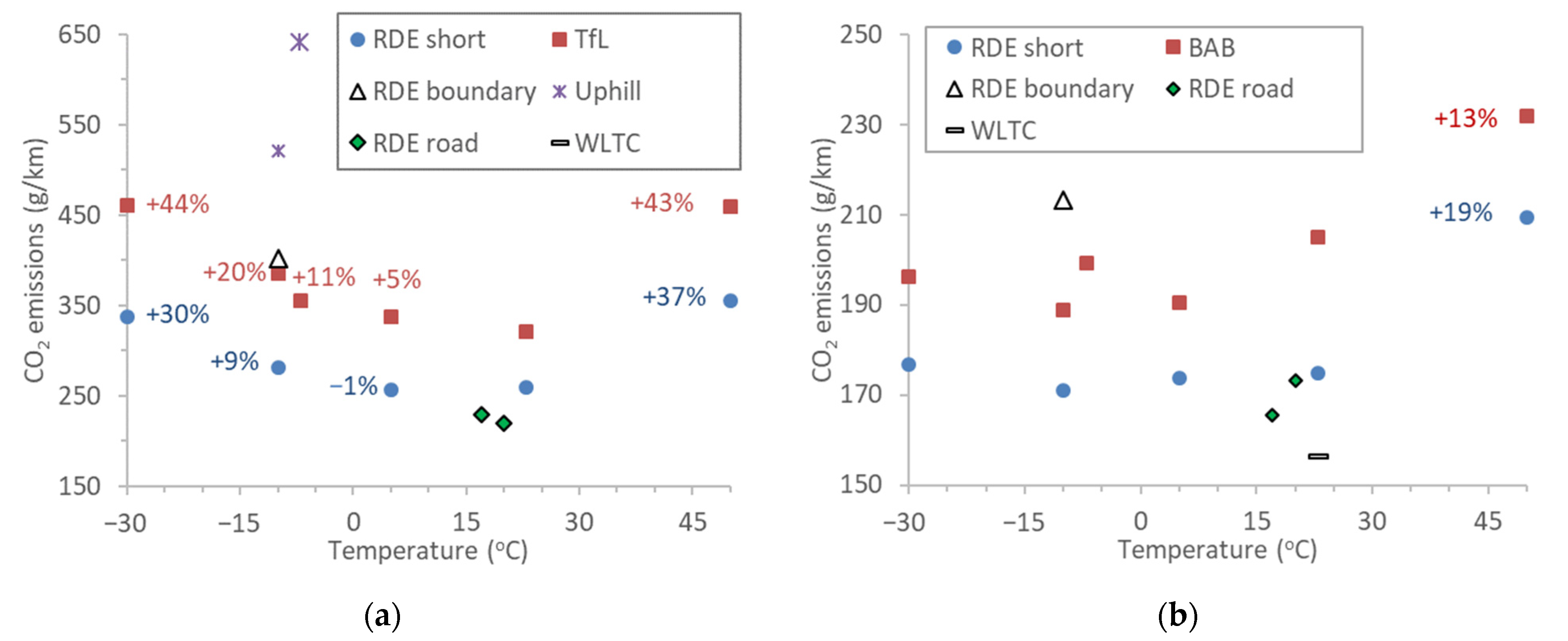
Figure 3 presents the CO2 emissions of the vehicle for the urban and motorway cycles. Starting with CO2 of urban cycles (Figure 3a), for the same cycle (e.g., RDE short or TfL), the emissions in function of the ambient temperature showed a bathtub-like curve. They were the lowest in the 5 °C to 23 °C range and increased at lower and higher ambient temperatures. The percentages give the CO2 increase compared to the 23 °C case, for cycles that different ambient temperature tests were available (TfL and RDE short). For example, at 50 °C, the CO2 was 43% higher compared to the 23 °C test for the TfL and +37% for the RDE short. The higher emission at low and high temperatures reflects the additional fuel consumption due to the use of the air-conditioning (A/C) system, while for the uphill cycles, additionally, the higher power demands due to the road grade and towing of the trailer. It should be mentioned that the road load coefficient F2 (a proxy for the airdrag coefficient) that was used with the chassis dynamometer was not corrected for the differences of air density at different temperatures. The effect should be negligible for the urban cycles.
For the same temperature (e.g., −10 °C and −7 °C) the highest values were noted for the uphill cycles towing a trailer, which required high engine power. Note that the uphill cycle with 85% towing (big symbol) had higher emissions than the 35% towing, even though the temperature was 3 degrees higher. The dynamic cycle RDE boundary and the congested traffic cycle TfL followed. RDE short had the lowest values. A similar trend was noted at 23 °C, but the cycles were more similar in terms of power demand (RDE road, RDE short).
Figure 3b summarises the motorway results. The differences were much smaller, within experimental uncertainties at the −30 °C to 23 °C temperature range. It should be mentioned though that the road load coefficients were not increased at lower temperatures (10% at −7 °C) as typically required in the regulations, and thus, the presented CO2 emissions at lower temperatures are underestimated. At 50 °C, there was a significant (around 15%) increase of the CO2.
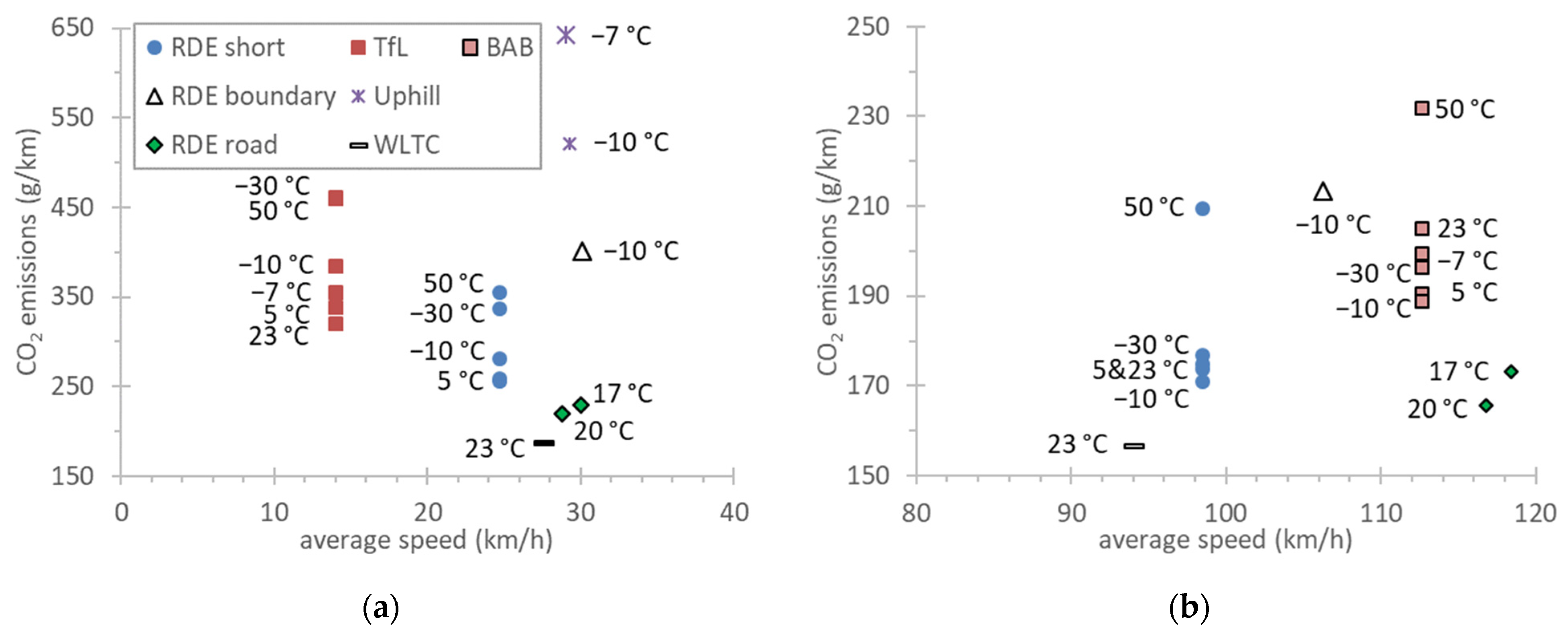
Figure 4 presents the correlation of CO2 with the mean speed for the urban cycles and the motorway cycles (Figure 4b). For urban cycles (Figure 4a), the emissions increase as the mean cycle speed decreases. However, there is still a temperature effect, as discussed previously. Most importantly there are a few points that do not follow the trendline: the uphill and dynamic cycles. For the motorway cycles (Figure 4b), there is no clear trend (note also the much smaller y-axis range). For the motorway cycles, the mean speed was between 95 km/h and 120 km/h. For the same ambient temperature, higher mean speed had slightly higher CO2 values (around +20 g/km), as expected due to the rapid increase in aerodynamic losses. With the exception of the 50°C tests, the rest results (−10 °C to 23 °C) for the same cycle (and mean speed) varied within a range of 10–20 g/km. The on-road tests, which had a mean speed close to 120 km/h had 20–30 g/km lower CO2 emissions than the BAB cycles. These results indicate an additional strong dependence on cycle dynamicity (e.g., aggressiveness of the cycle).
Figure 5 presents the correlation of CO2 with the 95th percentile of speed times acceleration (v × a). The left panel present the urban cycles, while the right panel the motorway cycles. This indicator is used in the RDE regulation to prevent extremely dynamic driving, that might have an impact on the emissions. Quite often, it is used as indicator of the trip dynamics. Figure 5 shows that for different urban cycles, v × a and CO2 do not have any correlation. One of the reasons is that v × a does not include road gradient, additional payload, or the use of air-conditioning (A/C), which have an impact on CO2 emissions. For the motorway cycles, for the same ambient temperature (e.g., −10 °C), the correlation is weak.
Figure 6a plots the cumulative CO2 emissions as a function of the positive work at the wheels as calculated from Equation (6), for different cycles and their phases (urban, rural, motorway). There is a linear correlation between the two variables for the different cycles, even though the scatter of some points (e.g., TfL) around the mean is quite large.
Figure 6b plots the CO2 emissions as a function of the distance related cycle energy (DrCE). Practically it is similar to Figure 6a, dividing every point with the distance of the specific test. However, the correlation does not improve compared to Figure 6a, but slightly gets worse. It should be recalled that the work and DrCE practically reflect the cycle demands (see Equations (5) and (8)), while the CO2 emissions correspond to the fuel consumed, which depends, in addition to the cycle demands, on auxiliary and air conditioning power demands and the combustion (engine) losses. The contribution of each parameter will be analysed in the Discussions section.

4. Discussion

This study assessed the CO2 emissions of a Euro 6d-temp gasoline vehicle with TWC and GPF, focusing on extreme temperatures and driving conditions. The major contribution of this study is the extension to extreme ambient temperatures (−30 °C and 50 °C) and driving conditions (congested traffic, dynamic driving, towing 85% of the max trailer load). In many cases, the correlation of CO2 cycle emissions to various parameters (e.g., average speed [38,39], speed times acceleration [59]) was weak in agreement with other researchers. To better understand the results, simulations were performed to quantify the contribution of various parameters on energy consumption and CO2.

4.1. Fuel Energy Shares

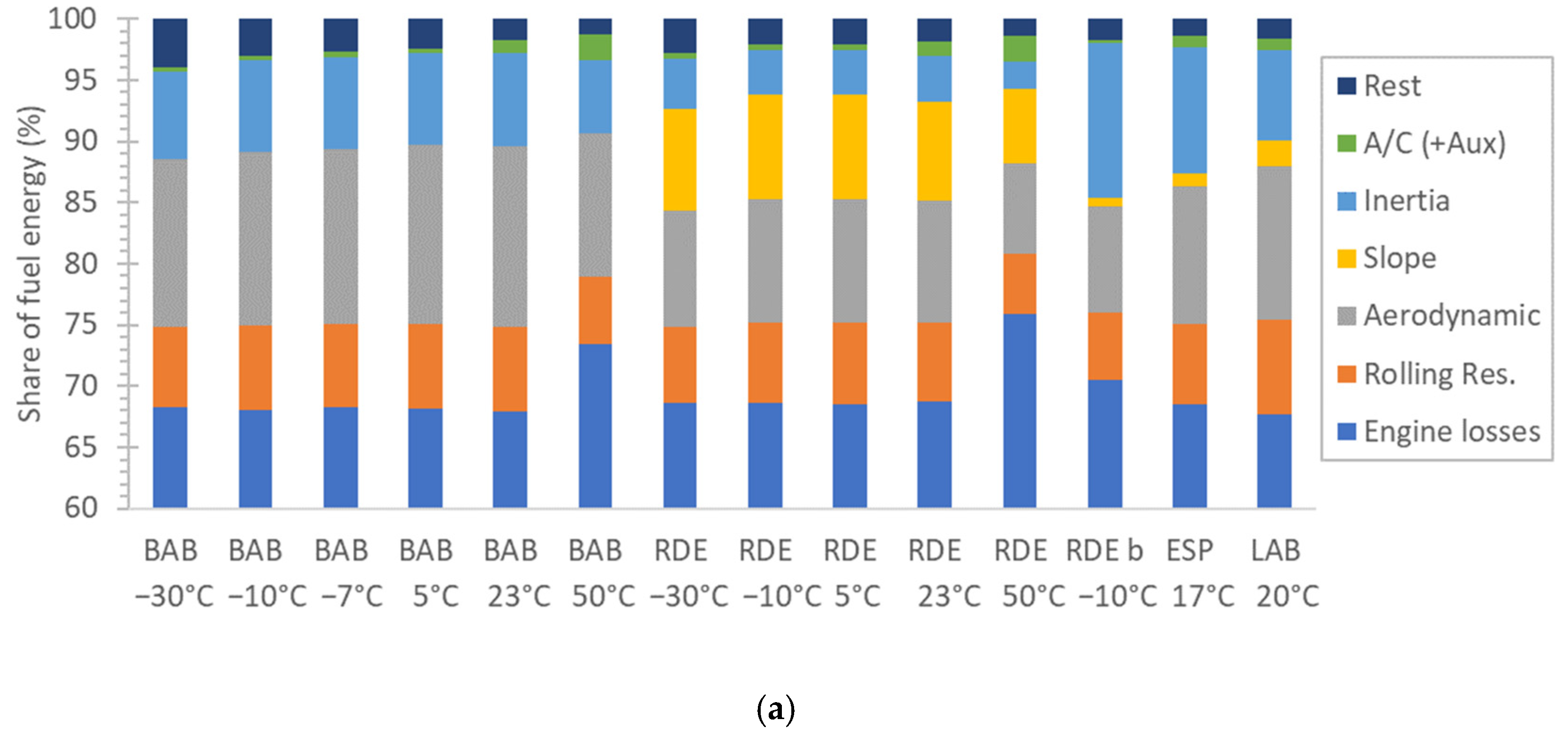
Figure 7 presents the relative contribution of various parameters to the final energy consumption (fuel energy), based on the simulation tool. Each cycle at each temperature is presented separately. Figure 7a plots the motorway cycle BAB or the motorway parts of the other cycles. The lost energy is 69–75%, with the highest values at the 50 °C tests. This has to do with the more frequent fuel enrichments under these conditions. The contribution of rolling resistance losses (F0RRR) was on average 7% and of aerodynamic resistance (F2Rd) 12%. The slope contribution was 8% for the RDE short and 2% for the RDE road. BAB had no slope. The contribution of A/C was slightly higher than 2% for the 50 °C tests and half (around 1%) for the 23 °C tests. The reason is that the air-conditioning load was minimum below 20 °C and was increasing with higher ambient temperatures. The rest losses were 1.4–4.1% (higher for low ambient temperatures).
Figure 7b plots the urban cycles or the urban parts of the RDE cycles. The lost energy is 70–84%, with the highest values in the low ambient temperature tests, due to the higher contribution of cold start (lower efficiency in the gearbox, torque converter, extended warm up phase). The TfL had also higher losses than the rest cycles. The urban cycles’ relative energy loss was higher than the motorway cycles (Figure 7a). In urban cycles, cold start was the contributing factor, while in motorway cycles, the fuel enrichment. For this reason, the trend was the opposite: urban cycles had higher lost energy with decreasing temperature, while motorway cycles, high ambient temperature. The contribution of rolling resistance losses (F0RRR) was on average 3.4% and of aerodynamic resistance (F2Rd) 0.6% (due to the low speeds). The contribution of A/C was 5–7% for the 50 °C tests. For the uphill tests, the contribution of slope was around 15%, it being the dominant source of energy consumption. For the rest cycles the contribution was much smaller (2% for RDE sort, 4.5% for RDE road).
The indicative engine efficiency, defined as the ratio of the positive engine work to the fuel energy content, can be calculated from the data above as one minus the engine losses. It was on average about 30% for the motorway cycles, while for the urban cycles, on average, 23% exhibited high cycle dependency. The complete cycles had an efficiency ranging from 24% to 30%, with an average of 27%. Analysing the chassis dyno test results, we see that the average indicative vehicle efficiency of the different cycles, i.e., the ratio between the total energy at the wheel and the total fuel energy content, is of the order of 25%, a value relatively high compared to past literature values. This positive finding reflects an overall improvement of vehicle and powertrain efficiency. Modelling results for WLTP indicate similar vehicle efficiency (26%) and average engine efficiency of approximately 31%. A 3–5% difference between indicative vehicle and engine efficiencies can be explained by the additional work provided by the engine for auxiliaries (e.g., A/C), which is not considered when calculating vehicle-related values.

4.2. Sensitivity Analysis

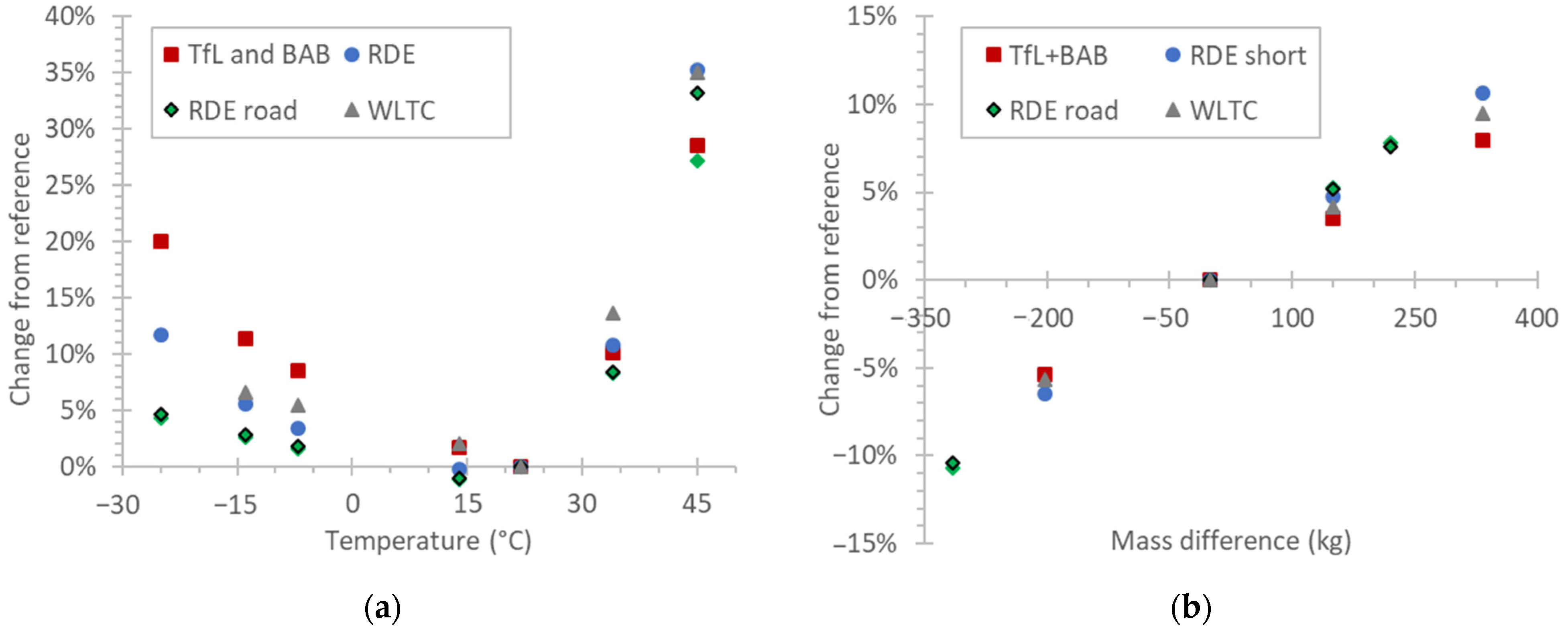
Figure 8a presents the CO2 sensitivity to ambient temperature for various cycles, keeping the rest parameters the same (as described in the experimental part). The 23 °C were considered the basis in the comparison. There is a significant increase (10% at 35 °C and 30% at 45 °C) due to the A/C use and the enrichment at high loads. The scatter of the differences at a specific temperature (e.g., 27–35% at 45 °C) has to do with the speed profile and duration of the cycles. At lower temperatures, there is an increase in CO2 emissions (between 5 and 20% at −25 °C), mainly due to the higher contribution of cold start. Studies have reported a 25% increase of CO2 from 23 °C to −7 °C in the urban part of the type approval cycle (NEDC), while for the complete cycle the effect was 17% [60]. Another study with Euro 6 vehicles found changes ranging up to 23% [61].
Many studies have found higher emissions due to lower ambient temperatures [62]. The main reason of higher emissions is high viscosity and friction; but excess fuelling contributes as well [63]. A study found +100 to +400 g CO2 when the temperature decreased from 23 °C to −20 °C [64]. In our tests, an increase of 30–44% (78–140 g/km CO2) was measured when the ambient temperature changed from 23 °C to −30 °C, even though the road load coefficients remained the same.
At high temperatures, in addition to the fuel enrichment, the energy consumption from the A/C is significant. In one study, switching on the A/C resulted on average +40 g/km (12%) extra CO2 emissions [65]. Furthermore, the higher the ambient air temperature, the higher the CO2 emissions were. Most studies in the literature showed a 15–25% increase with the use of A/C [66]. A dedicated study found +30 g/km or +10% as the contribution of A/C when the ambient temperature was 37°C instead of 23°C in an urban cycle [65]. That was the average of five cars; the maximum increase was +82.7 g/km (+26%). In another study, the increase from A/C use was 90% while idle, and it decreased from 35% to 9% at constant speed as speed increased [51]. An effect of up to 28% has also been shown for hybrid vehicles [67].
Figure 8b plots the effect of additional or less mass on the CO2. The effect is linear with a slope of 3% every 100 kg. This increase is in line with the findings of another simulation based study [68,69]. Several studies exist in the literature about the impact of the additional mass in CO2. One study reports less impact [70] and others higher. For example, a 230 kg increase (+17%) resulted in 10–20% higher CO2 emissions [71]. In a review paper, 5–7% increase of the CO2 for every 100 kg increase of the vehicle mass was found [66].
Figure 9a summarizes the simulation results modifying the original slope by up to ±70% for the RDE short cycle with slope simulated by the dyno or the actual on-road tests RDE road. These two RDE cycles had a natural variable positive and negative slope over the trip, while the TfL and WLTC had no slope. For the last two cycles, a constant slope was added or subtracted for the simulations (±2%) (Figure 9b). A +50% for the RDE means 50% increase of the actual positive slope, e.g., 5% slope would be 7.5%, but a −5% slope in the same trip would be −7.5%. A −50% for the RDE means 50% decrease of the actual positive slope, e.g., 5% slope would be 2.5%, but a -5% slope in the same trip would be −2.5%.
The effect on the RDE (short and road) cycles was ±10% (Figure 9a), while for the rest cycles with a fixed slope addition the effect was up to ±30%. For the limited variations of road gradient simulated here, the effect on CO2 emissions was almost linear. The literature suggests a 5–9% increase for a 1–1.5% slope [14], and 40–100% for a 5% slope [20,72,73].
Simulations of the RDE cycles were performed across the full range of ambient temperature (as in Figure 8a) and for changes of the slope up to ±70% (as in Figure 9a). The different slopes resulted in a different average positive motive power across the trips. Based on these results, we introduce in Figure 10 a 3-dimension presentation of the simulated CO2 percentage difference from the 23 °C WLTC value as a function of the ambient temperature and the change of the mean positive power at the wheel (WLTC taken as reference). Only the RDE cycles performed in the laboratory and on road were simulated because they had a realistic elevation pattern. Thus, Figure 10 is a combination of Figure 8a and Figure 9a but within the entire temperature and slope simulated range.
RDE short (laboratory) and RDE road 1 (on-road) with the original slope had on average 25% higher positive motive power than on WLTC test. RDE road 2 (test on-road) had an average difference of 35% due to its trip characteristics. Smaller differences (but still positive) were simulated with the “negative” slope. Overall, the difference of the positive motive power from WLTC ranged from 5 to 60% and maintained a quasi-linear profile. The additional CO2 increase ranges from 15 to 30% with the additional positive power.
A second order polynomial model was selected to fit the additional CO2 as a function of the ambient temperature, with its minimum at 14 °C (11–15% depending on the trip) for the base simulation (use of original slope). The lowest CO2 difference at 14 °C can be justified due to the reduced needs for cabin heating and cooling and the fact that the official WLTP CO2 emissions certification value is declared after being corrected for 14 °C conditions. The highest difference in the original slope was seen at the highest ambient temperature (45 °C, 50% average difference from WLTC) caused by the excessive needs for air-conditioning (A/C) and other reasons described previously. In the lowest ambient temperature, the increase was again significant (−25 °C, 22% average difference from WLTC). The message from this figure is that the slope or ambient temperature effects are not only cycle dependent (as it was shown in Figure 8a and Figure 9a), but there is a combined effect (e.g., higher slopes at higher temperatures might need more fuel enrichment). The fit is given in Equation (9). The R2 value was 0.813, which implies an acceptable correlation.
Δ CO 2 = ( c 1 · Δ P + + c 2 ) ·   ( c 3 · T amb 2 + c 4   · T amb + c 5 )
where ΔCO2 [%] is the CO2 difference from WLTC (values 0–100), ΔP+ [%] is the mean positive motive power difference from WLTC (values 0–100), Tamb [°C] is the mean ambient temperature. The constants are c1 = 0.0001269, c2 = 0.003989, c3 = 2.467, c4 = −11.74, and c5 = 1487.

5. Conclusions

A Euro 6d-Temp gasoline direct injection (GDI) vehicle was tested on the road and in the laboratory with cycles simulating congested urban traffic, uphill driving towing a trailer at 85% of the maximum payload of the car and the trailer, and dynamic driving at ambient temperatures between −30 °C to 50 °C. In urban trips, compared to the baseline at 23 °C, the CO2 emissions were 9–20% higher at −10 °C, 30–44% higher at −30 °C, and 37–43% higher at 50 °C. Uphill driving with trailer had 2–3 times higher CO2 emissions. In motorway trips, the CO2 was higher 13–19% only at the 50 °C ambient temperature. The CO2 emissions did not show any particular trend in function of trip average speed because the contributions of the ambient temperature and payload were higher. The simulations of the trips with CO2MPAS were on average within ±5%, with a few exceptions (50 °C and uphill driving with trailer) where the differences were 5–12%. The simulation tool was used to predict the effect of ambient temperature, vehicle mass, and road grade on the CO2 emissions. The simulations gave an almost linear and proportional effect of 3.5% every 100 kg increase of the vehicle weight, and a 12–14% increase for every grade of slope. The temperature effect was not linear, but with small uncertainties, an increase of 15 °C or a decrease of 15 °C of the ambient temperature resulted in a 7–15% increase of the CO2 emissions, with the higher values at traffic and high ambient temperatures.

Author Contributions

Conceptualization, G.F.; formal analysis, B.G. and D.K.; writing—original draft preparation, B.G. and D.K.; writing—review and editing, G.F. All authors have read and agreed to the published version of the manuscript.

Funding

This research received no external funding.

Institutional Review Board Statement

Not applicable.

Informed Consent Statement

Not applicable.

Data Availability Statement

The data are available upon request from the corresponding authors.

Acknowledgments

The authors would like to acknowledge the VELA staff (M. Otura, C. Ferrarese, F. Forloni) for the experimental support.

Conflicts of Interest

The authors declare no conflict of interest. The opinions expressed in this manuscript are those of the authors and should in no way be considered to represent an official opinion of the European Commission. Mention of trade names or commercial products does not constitute endorsement or recommendation by the European Commission or the authors.

Appendix A

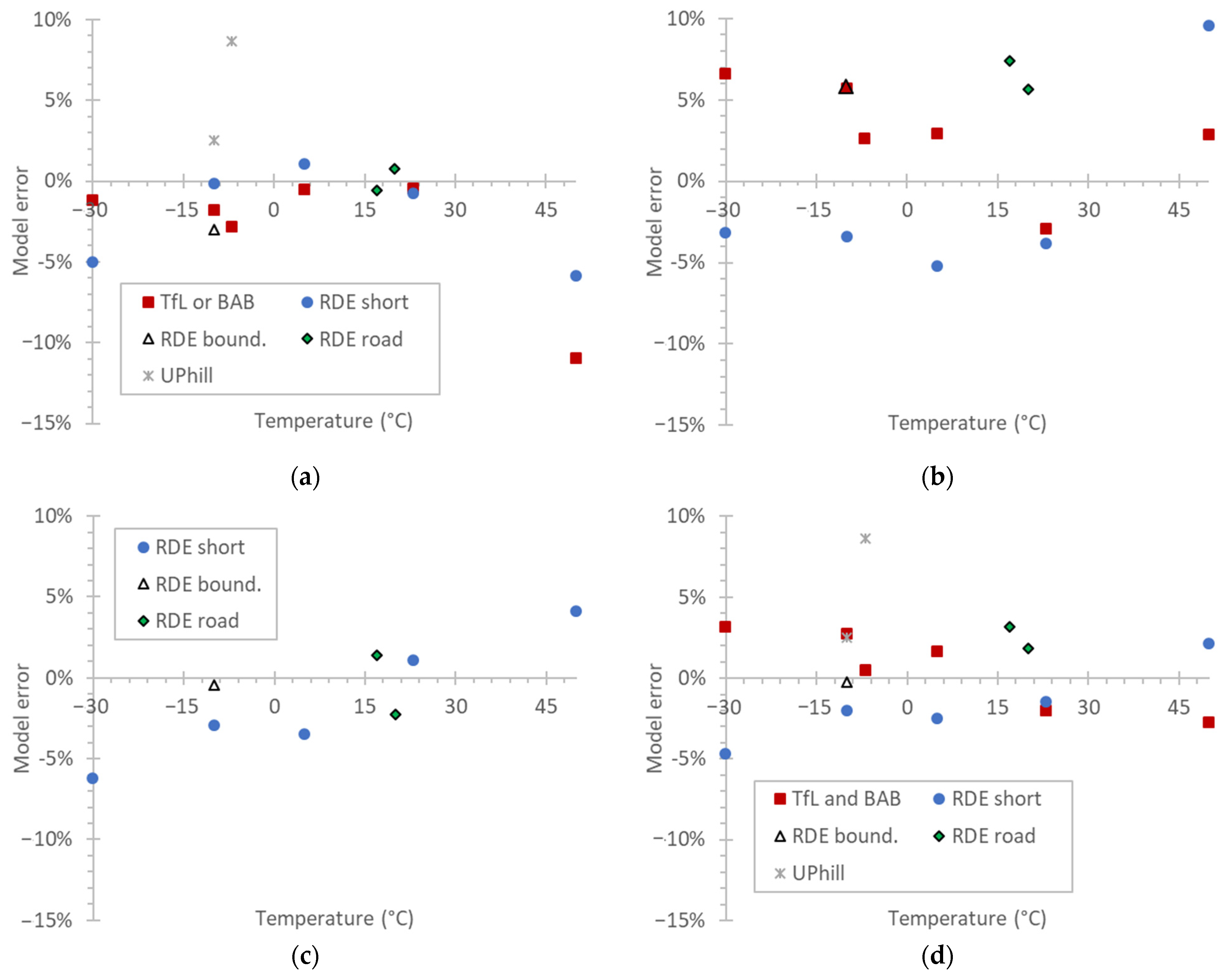
Figure A1 plots the model error as function of the ambient temperature for various cycles at urban (Figure A1a), motorway (Figure A1b), rural (Figure A1c) parts, and complete trip (Figure A1d). In general, there is a good agreement between experimental and modelled results, giving confidence about the assumptions made. The mean difference is −1.2% (±4.7%) for the urban cycles, 2.1% (±3.8%) for motorway cycles, −1.1% (±3.3%) for rural cycles, and 0.7% (±3.2%) for the complete trips. The higher differences were found for the high temperature (50°C) tests and the uphill cycles. The higher differences for the uphill cycles come from the first 200 s, because the model could not predict accurately the engine coolant temperature. At high ambient temperatures, there is a slight CO2 underprediction in the urban parts (Figure A1a) and overprediction in the motorway parts (Figure A1b). Still, in RDE short that incorporates a rural part, the model had a good agreement (Figure A1c,d). Overall, the models created to capture the high temperature tests show reasonable error figures, pointing out the need for further improvements in the A/C operation and the fuel enrichments.
Figure A1. Model error at (a) urban cycles (TfL, uphill) or urban parts of other cycles, (b) motorway cycles (BAB) or motorway part of other cycles, (c) rural parts, and (d) complete cycle.
Energies 14 06195 g0a1

References

  1. West, J.J.; Smith, S.J.; Silva, R.A.; Naik, V.; Zhang, Y.; Adelman, Z.; Fry, M.M.; Anenberg, S.; Horowitz, L.W.; Lamarque, J.-F. Co-Benefits of Mitigating Global Greenhouse Gas Emissions for Future Air Quality and Human Health. Nat. Clim. Chang. 2013, 3, 885–889. [Google Scholar] [CrossRef] [PubMed] [Green Version]
  2. Woodward, A.; Baumgartner, J.; Ebi, K.L.; Gao, J.; Kinney, P.L.; Liu, Q. Population Health Impacts of China’s Climate Change Policies. Environ. Res. 2019, 175, 178–185. [Google Scholar] [CrossRef]
  3. European Commission. Transport Emissions: A European Strategy for Low-Emission Mobility 2021. Available online: https://ec.europa.eu/clima/policies/transport_en (accessed on 27 September 2021).
  4. Pavlovic, J.; Fontaras, G.; Ktistakis, M.; Anagnostopoulos, K.; Komnos, D.; Ciuffo, B.; Clairotte, M.; Valverde, V. Understanding the Origins and Variability of the Fuel Consumption Gap: Lessons Learned from Laboratory Tests and a Real-Driving Campaign. Environ. Sci. Eur. 2020, 32, 53. [Google Scholar] [CrossRef] [Green Version]
  5. Pavlovic, J.; Anagnostopoulos, K.; Clairotte, M.; Arcidiacono, V.; Fontaras, G.; Rujas, I.P.; Morales, V.V.; Ciuffo, B. Dealing with the Gap between Type-Approval and in-Use Light Duty Vehicles Fuel Consumption and CO2 Emissions: Present Situation and Future Perspective. Transp. Res. Rec. 2018, 2672, 23–32. [Google Scholar] [CrossRef]
  6. Tietge, U.; Díaz, S.; Mock, P.; Bandivadekar, A.; Dornoff, J.; Ligterink, N. From Laboratoy to Road: A 2018 Update of Official and Real-World Fuel Consumption and CO2 Values for Passenger Cars in Europe; ICCT: Berlin, Germany, 2019. [Google Scholar]
  7. Pavlovic, J.; Ciuffo, B.; Fontaras, G.; Valverde, V.; Marotta, A. How Much Difference in Type-Approval CO2 Emissions from Passenger Cars in Europe Can Be Expected from Changing to the New Test Procedure (NEDC vs. WLTP)? Transp. Res. Part A Policy Pract. 2018, 111, 136–147. [Google Scholar] [CrossRef]
  8. Chatzipanagi, A.; Pavlovic, J.; Fontaras, G.; Komnos, D. Impact of WLTP Introduction on CO2 Emissions from M1 and N1 Vehicles: Evidence from Type-Approval and 2018 EEA Data; Publications Office of the European Union: Luxembourg, 2020; ISBN 978-92-76-22766-3. [Google Scholar] [CrossRef]
  9. Pavlovic, J.; Fontaras, G.; Broekaert, S.; Ciuffo, B.; Ktistakis, M.A.; Grigoratos, T. How Accurately Can We Measure Vehicle Fuel Consumption in Real World Operation? Transp. Res. Part D Transp. Environ. 2021, 90, 102666. [Google Scholar] [CrossRef]
  10. Ktistakis, M.A.; Pavlovic, J.; Fontaras, G. Sampling Approaches for Road Vehicle Fuel Consumption Monitoring; Report EUR 30420 EN; Publications Office of the European Union: Luxembourg, 2021. [Google Scholar]
  11. Reksowardojo, I.K.; Setiapraja, H.; Fajar, R.; Wibowo, E.; Kusdiana, D. An Investigation of Laboratory and Road Test of Common Rail Injection Vehicles Fueled with B20 Biodiesel. Energies 2020, 13, 6118. [Google Scholar] [CrossRef]
  12. Tucki, K.; Orynycz, O.; Mitoraj-Wojtanek, M. Perspectives for Mitigation of CO2 Emission Due to Development of Electromobility in Several Countries. Energies 2020, 13, 4127. [Google Scholar] [CrossRef]
  13. Sendek-Matysiak, E.; Łosiewicz, Z. Analysis of the Development of the Electromobility Market in Poland in the Context of the Implemented Subsidies. Energies 2021, 14, 222. [Google Scholar] [CrossRef]
  14. Fontaras, G.; Zacharof, N.-G.; Ciuffo, B. Fuel Consumption and CO2 Emissions from Passenger Cars in Europe—Laboratory versus Real-World Emissions. Prog. Energy Combust. Sci. 2017, 60, 97–131. [Google Scholar] [CrossRef]
  15. Wen, Y.; Zhang, S.; He, L.; Yang, S.; Wu, X.; Wu, Y. Characterizing Start Emissions of Gasoline Vehicles and the Seasonal, Diurnal and Spatial Variabilities in China. Atmos. Environ. 2021, 245, 118040. [Google Scholar] [CrossRef]
  16. Al-Wreikat, Y.; Serrano, C.; Sodré, J.R. Driving Behaviour and Trip Condition Effects on the Energy Consumption of an Electric Vehicle under Real-World Driving. Appl. Energy 2021, 297, 117096. [Google Scholar] [CrossRef]
  17. Kim, S.; Jeong, H.; Lee, H. Cold-Start Performance Investigation of Fuel Cell Electric Vehicles with Heat Pump-Assisted Thermal Management Systems. Energy 2021, 232, 121001. [Google Scholar] [CrossRef]
  18. Weller, K.; Lipp, S.; Röck, M.; Matzer, C.; Bittermann, A.; Hausberger, S. Real World Fuel Consumption and Emissions From LDVs and HDVs. Front. Mech. Eng. 2019, 5, 45. [Google Scholar] [CrossRef] [Green Version]
  19. Yang, B.; Yao, M.; Li, X.; Wang, M.; Wei, D.; Li, G. Impact of Thermal Architecture on Electric Vehicle Energy Consumption/Range: A Study with Full Vehicle Simulation; SAE Technical Paper 2021-01-0207; SAE: Warrendale, PA, USA, 2021. [Google Scholar] [CrossRef]
  20. Gao, J.; Chen, H.; Dave, K.; Chen, J.; Jia, D. Fuel Economy and Exhaust Emissions of a Diesel Vehicle under Real Traffic Conditions. Energy Sci. Eng. 2020, 8, 1781–1792. [Google Scholar] [CrossRef]
  21. Zachiotis, A.T.; Giakoumis, E.G. Monte Carlo Simulation Methodology to Assess the Impact of Ambient Wind on Emissions from a Light-Commercial Vehicle Running on the Worldwide-Harmonized Light-Duty Vehicles Test Cycle (WLTC). Energies 2021, 14, 661. [Google Scholar] [CrossRef]
  22. Wyatt, D.W.; Li, H.; Tate, J.E. The Impact of Road Grade on Carbon Dioxide (CO2) Emission of a Passenger Vehicle in Real-World Driving. Transp. Res. Part D Transp. Environ. 2014, 32, 160–170. [Google Scholar] [CrossRef] [Green Version]
  23. Costagliola, M.A.; Costabile, M.; Prati, M.V. Impact of Road Grade on Real Driving Emissions from Two Euro 5 Diesel Vehicles. Appl. Energy 2018, 231, 586–593. [Google Scholar] [CrossRef]
  24. Zachiotis, A.T.; Giakoumis, E.G. Methodology to Estimate Road Grade Effects on Consumption and Emissions from a Light Commercial Vehicle Running on the WLTC Cycle. J. Energy Eng. 2020, 146, 04020048. [Google Scholar] [CrossRef]
  25. Jiménez, J.L.; Valido, J.; Molden, N. The Drivers behind Differences between Official and Actual Vehicle Efficiency and CO2 Emissions. Transp. Res. Part D Transp. Environ. 2019, 67, 628–641. [Google Scholar] [CrossRef]
  26. Küng, L.; Bütler, T.; Georges, G.; Boulouchos, K. How Much Energy Does a Car Need on the Road? Appl. Energy 2019, 256, 113948. [Google Scholar] [CrossRef]
  27. Franco, V.; Kousoulidou, M.; Muntean, M.; Ntziachristos, L.; Hausberger, S.; Dilara, P. Road Vehicle Emission Factors Development: A Review. Atmos. Environ. 2013, 70, 84–97. [Google Scholar] [CrossRef]
  28. Valverde, V.; Mora, B.A.; Clairotte, M.; Pavlovic, J.; Suarez-Bertoa, R.; Giechaskiel, B.; Astorga-LLorens, C.; Fontaras, G. Emission Factors Derived from 13 Euro 6b Light-Duty Vehicles Based on Laboratory and on-Road Measurements. Atmosphere 2019, 10, 243. [Google Scholar] [CrossRef] [Green Version]
  29. Valverde-Morales, V.; Clairotte, M.; Pavlovic, J.; Giechaskiel, B.; Bonnel, P. On-Road Emissions of Euro 6d-TEMP Vehicles: Consequences of the Entry into Force of the RDE Regulation in Europe; SAE Technical Paper 2020-01-2219; SAE: Warrendale, PA, USA, 2020. [Google Scholar] [CrossRef]
  30. Nesamani, K.S.; Saphores, J.-D.; McNally, M.G.; Jayakrishnan, R. Estimating Impacts of Emission Specific Characteristics on Vehicle Operation for Quantifying Air Pollutant Emissions and Energy Use. J. Traffic Transp. Eng. 2017, 4, 215–229. [Google Scholar] [CrossRef]
  31. Yu, Q.; Yang, Y.; Xiong, X.; Sun, S.; Liu, Y.; Wang, Y. Assessing the Impact of Multi-Dimensional Driving Behaviors on Link-Level Emissions Based on a Portable Emission Measurement System (PEMS). Atmos. Pollut. Res. 2021, 12, 414–424. [Google Scholar] [CrossRef]
  32. Kuhler, M.; Karstens, D. Improved Driving Cycle for Testing Automotive Exhaust Emissions; SAE Technical Paper 780650; SAE: Warrendale, PA, USA, 1978. [Google Scholar] [CrossRef]
  33. Ericsson, E. Independent Driving Pattern Factors and Their Influence on Fuel-Use and Exhaust Emission Factors. Transp. Res. Part D Transp. Environ. 2001, 6, 325–345. [Google Scholar] [CrossRef]
  34. Rakha, H.; Ahn, K.; Trani, A. Development of VT-Micro Model for Estimating Hot Stabilized Light Duty Vehicle and Truck Emissions. Transp. Res. Part D Transp. Environ. 2004, 9, 49–74. [Google Scholar] [CrossRef]
  35. Wang, H.; Fu, L.; Zhou, Y.; Li, H. Modelling of the Fuel Consumption for Passenger Cars Regarding Driving Characteristics. Transp. Res. Part D Transp. Environ. 2008, 13, 479–482. [Google Scholar] [CrossRef]
  36. Oduro, S.D.; Metia, S.; Duc, H.; Ha, Q.P. CO2 Vehicular Emission Statistical Analysis with Instantaneous Speed and Acceleration as Predictor Variables. In Proceedings of the 2013 International Conference on Control, Automation and Information Sciences (ICCAIS), Nha Trang, Vietnam, 25–28 November 2013; pp. 158–163. [Google Scholar]
  37. Afotey, B.; Sattler, M.; Mattingly, S.P.; Chen, V.C.P. Statistical Model for Estimating Carbon Dioxide Emissions from a Light-Duty Gasoline Vehicle. JEP 2013, 4, 8–15. [Google Scholar] [CrossRef] [Green Version]
  38. Rodríguez, R.A.; Virguez, E.A.; Rodríguez, P.A.; Behrentz, E. Influence of Driving Patterns on Vehicle Emissions: A Case Study for Latin American Cities. Transp. Res. Part D Transp. Environ. 2016, 43, 192–206. [Google Scholar] [CrossRef]
  39. Qu, L.; Wang, W.; Li, M.; Xu, X.; Shi, Z.; Mao, H.; Jin, T. Dependence of Pollutant Emission Factors and Fuel Consumption on Driving Conditions and Gasoline Vehicle Types. Atmos. Pollut. Res. 2021, 12, 137–146. [Google Scholar] [CrossRef]
  40. Barth, M.; Boriboonsomsin, K. Energy and Emissions Impacts of a Freeway-Based Dynamic Eco-Driving System. Transp. Res. Part D Transp. Environ. 2009, 14, 400–410. [Google Scholar] [CrossRef]
  41. Frey, H.C.; Zhang, K.; Rouphail, N.M. Fuel Use and Emissions Comparisons for Alternative Routes, Time of Day, Road Grade, and Vehicles Based on in-Use Measurements. Environ. Sci. Technol. 2008, 42, 2483–2489. [Google Scholar] [CrossRef] [PubMed]
  42. Sentoff, K.M.; Aultman-Hall, L.; Holmén, B.A. Implications of Driving Style and Road Grade for Accurate Vehicle Activity Data and Emissions Estimates. Transp. Res. Part D Transp. Environ. 2015, 35, 175–188. [Google Scholar] [CrossRef]
  43. Cubito, C.; Millo, F.; Boccardo, G.; Di Pierro, G.; Ciuffo, B.; Fontaras, G.; Serra, S.; Otura Garcia, M.; Trentadue, G. Impact of Different Driving Cycles and Operating Conditions on CO2 Emissions and Energy Management Strategies of a Euro-6 Hybrid Electric Vehicle. Energies 2017, 10, 1590. [Google Scholar] [CrossRef]
  44. Giechaskiel, B.; Valverde, V.; Kontses, A.; Melas, A.; Martini, G.; Balazs, A.; Andersson, J.; Samaras, Z.; Dilara, P. Particle Number Emissions of a Euro 6d-Temp Gasoline Vehicle under Extreme Temperatures and Driving Conditions. Catalysts 2021, 11, 607. [Google Scholar] [CrossRef]
  45. Fontaras, G.; Valverde, V.; Arcidiacono, V.; Tsiakmakis, S.; Anagnostopoulos, K.; Komnos, D.; Pavlovic, J.; Ciuffo, B. The Development and Validation of a Vehicle Simulator for the Introduction of Worldwide Harmonized Test Protocol in the European Light Duty Vehicle CO2 Certification Process. Appl. Energy 2018, 226, 784–796. [Google Scholar] [CrossRef]
  46. Mogno, C.; Fontaras, G.; Arcidiacono, V.; Komnos, D.; Pavlovic, J.; Ciuffo, B.; Makridis, M.; Valverde, V. The Application of the CO2MPAS Model for Vehicle CO2 Emissions Estimation over Real Traffic Conditions. Transp. Policy 2020. [Google Scholar] [CrossRef]
  47. Joachim, F.J.; Börner, J.; Kurz, N. How to Minimize Power Losses in Transmissions, Axles and Steering Systems. Gear Technol. 2012, 2012, 58–66. [Google Scholar]
  48. Gillot, R.; Dempsey, M.; Picarelli, A. Predicting the Effect of Powertrain Preconditioning on Vehicle Efficiency. Math. Comput. Model. Dyn. Syst. 2017, 23, 301–318. [Google Scholar] [CrossRef] [Green Version]
  49. Organisciak, M.; Baart, P.; Barbera, S.; Paykin, A.; Schweig, M. Theoretical and Experimental Study of the Frictional Losses of Radial Shaft Seals for Industrial Gearbox. Power Transm. Eng. 2015, 2015, 58–63. [Google Scholar]
  50. Fayazbakhsh, M.A.; Bahrami, M. Comprehensive Modeling of Vehicle Air Conditioning Loads Using Heat Balance Method; SAE Technical Paper 2013-01-1507; SAE: Warrendale, PA, USA, 2013. [Google Scholar] [CrossRef] [Green Version]
  51. Lee, J.; Kim, J.; Park, J.; Bae, C. Effect of the Air-Conditioning System on the Fuel Economy in a Gasoline Engine Vehicle. Proc. Inst. Mech. Eng. Part D J. Automob. Eng. 2013, 227, 66–77. [Google Scholar] [CrossRef]
  52. Mebarki, B.; Draoui, B.; Allaou, B.; Rahmani, L.; Benachour, E. Impact of the Air-Conditioning System on the Power Consumption of an Electric Vehicle Powered by Lithium-Ion Battery. Model. Simul. Eng. 2013, 2013, 1–6. [Google Scholar] [CrossRef] [Green Version]
  53. Galindo, E.; Blanco, D.; Brace, C.; Chappell, E.; Burke, R. Chassis Dynamometer Testing: Addressing the Challenges of New Global Legislation (WLTP and RDE); SAE International: Warrendale, PA, USA, 2017; ISBN 978-0-7680-8278-4. [Google Scholar]
  54. Farrington, R.; Rugh, J. Impact of Vehicle Air-Conditioning on Fuel Economy, Tailpipe Emissions, and Electric Vehicle Range; National Renewable Energy Lab. (NREL): Golden, CO, USA, 2000. [Google Scholar]
  55. Giechaskiel, B.; Valverde, V.; Kontses, A.; Suarez-Bertoa, R.; Selleri, T.; Melas, A.; Otura, M.; Ferrarese, C.; Martini, G.; Balazs, A.; et al. Effect of Extreme Temperatures and Driving Conditions on Gaseous Pollutants of a Euro 6d-Temp Gasoline Vehicle. Atmosphere 2021, 12, 1011. [Google Scholar] [CrossRef]
  56. Kühlwein, J. Driving Resistances of Light-Duty Vehicles in Europe: Present Situation, Trends, and Scenarios for 2025; ICCT: Berlin, Germany, 2016. [Google Scholar]
  57. Komnos, D.; Broekaert, S.; Grigoratos, T.; Ntziachristos, L.; Fontaras, G. In Use Determination of Aerodynamic and Rolling Resistances of Heavy-Duty Vehicles. Sustainability 2021, 13, 974. [Google Scholar] [CrossRef]
  58. Claßen, J.; Pischinger, S.; Krysmon, S.; Sterlepper, S.; Dorscheidt, F.; Doucet, M.; Reuber, C.; Görgen, M.; Scharf, J.; Nijs, M.; et al. Statistically Supported Real Driving Emission Calibration: Using Cycle Generation to Provide Vehicle-Specific and Statistically Representative Test Scenarios for Euro 7. Int. J. Engine Res. 2020, 21, 1783–1799. [Google Scholar] [CrossRef]
  59. Song, J.; Cha, J. Analysis of Driving Dynamics Considering Driving Resistances in On-Road Driving. Energies 2021, 14, 3408. [Google Scholar] [CrossRef]
  60. Dardiotis, C.; Martini, G.; Marotta, A.; Manfredi, U.; European Commission; Joint Research Centre; Institute for Energy and Transport. Extension of Low Temperature Emission Test to Euro 6 Diesel Vehicle; Publications Office: Luxembourg, 2012; ISBN 978-92-79-25610-3. [Google Scholar]
  61. Suarez-Bertoa, R.; Astorga, C. Impact of Cold Temperature on Euro 6 Passenger Car Emissions. Environ. Pollut. 2018, 234, 318–329. [Google Scholar] [CrossRef] [PubMed]
  62. Bielaczyc, P.; Woodburn, J.; Szczotka, A. Low Ambient Temperature Cold Start Emissions of Gaseous and Solid Pollutants from Euro 5 Vehicles Featuring Direct and Indirect Injection Spark-Ignition Engines. SAE Int. J. Fuels Lubr. 2013, 6, 968–976. [Google Scholar] [CrossRef]
  63. Bielaczyc, P.; Szczotka, A.; Woodburn, J. An Overview of Cold Start Emissions from Direct Injection Spark-Ignition and Compression Ignition Engines of Light Duty Vehicles at Low Ambient Temperatures. Combust. Engines 2013, 154, 96–103. [Google Scholar] [CrossRef]
  64. Weilenmann, M.; Favez, J.-Y.; Alvarez, R. Cold-Start Emissions of Modern Passenger Cars at Different Low Ambient Temperatures and Their Evolution over Vehicle Legislation Categories. Atmos. Environ. 2009, 43, 2419–2429. [Google Scholar] [CrossRef]
  65. Weilenmann, M.F.; Vasic, A.-M.; Stettler, P.; Novak, P. Influence of Mobile Air-Conditioning on Vehicle Emissions and Fuel Consumption: A Model Approach for Modern Gasoline Cars Used in Europe. Environ. Sci. Technol. 2005, 39, 9601–9610. [Google Scholar] [CrossRef] [PubMed]
  66. Fontaras, G.; Ciuffo, B.; Zacharof, N.; Tsiakmakis, S.; Marotta, A.; Pavlovic, J.; Anagnostopoulos, K. The Difference between Reported and Real-World CO2 Emissions: How Much Improvement Can Be Expected by WLTP Introduction? Transp. Res. Procedia 2017, 25, 3933–3943. [Google Scholar] [CrossRef]
  67. Li, C.; Brewer, E.; Pham, L.; Jung, H. Reducing Mobile Air Conditioner (MAC) Power Consumption Using Active Cabin-Air-Recirculation in a Plug-in Hybrid Electric Vehicle (PHEV). WEVJ 2018, 9, 51. [Google Scholar] [CrossRef] [Green Version]
  68. Pavlovic, J.; Marotta, A.; Anagnostopoulos, K.; Tsiakmakis, S.; Ciuffo, B.; Fontaras, G.; Zacharof, N.G.; European Commission; Joint Research Centre. Review of in Use Factors Affecting the Fuel Consumption and CO2 Emissions of Passenger Cars; Publications Office: Luxembourg, 2016. [Google Scholar]
  69. Lee, H.; Lee, K. Comparative Evaluation of the Effect of Vehicle Parameters on Fuel Consumption under NEDC and WLTP. Energies 2020, 13, 4245. [Google Scholar] [CrossRef]
  70. Mellios, G.; Hausberger, S.; Keller, M.; Samaras, C.; Ntziachristos, L.; Dilara, P.; Fontaras, G.; European Commission; Joint Research Centre; Institute for Energy and Transport. Parameterisation of Fuel Consumption and CO2 Emissions of Passenger Cars and Light Commercial Vehicles for Modelling Purposes; Publications Office: Luxembourg, 2009; ISBN 978-92-79-21051-8. [Google Scholar]
  71. Giechaskiel, B.; Riccobono, F.; Vlachos, T.; Mendoza-Villafuerte, P.; Suarez-Bertoa, R.; Fontaras, G.; Bonnel, P.; Weiss, M. Vehicle Emission Factors of Solid Nanoparticles in the Laboratory and on the Road Using Portable Emission Measurement Systems (PEMS). Front. Environ. Sci. 2015, 3, 82. [Google Scholar] [CrossRef] [Green Version]
  72. Zhang, K.; Frey, H.C. Road Grade Estimation for On-Road Vehicle Emissions Modeling Using Light Detection and Ranging Data. J. Air Waste Manag. Assoc. 2006, 56, 777–788. [Google Scholar] [CrossRef]
  73. Gallus, J.; Kirchner, U.; Vogt, R.; Benter, T. Impact of Driving Style and Road Grade on Gaseous Exhaust Emissions of Passenger Vehicles Measured by a Portable Emission Measurement System (PEMS). Transp. Res. Part D Transp. Environ. 2017, 52, 215–226. [Google Scholar] [CrossRef]
Figure 1. TfL and BAB cycles at different ambient temperatures (−30 °C to 50 °C): (a) cumulative CO2 emissions (the inset focuses on the first 600 s) and (b) cabin temperature.
Energies 14 06195 g001
Figure 2. Various cycles at −7 °C and −10 °C. Asterisk indicates the point at which a distance of approximately 9 km is covered (a) in function of time and (b) in function of cumulative positive power.
Energies 14 06195 g002
Figure 3. CO2 emissions of in function of ambient temperature: (a) urban cycles (TfL, uphill) or urban parts of the rest cycles (RDE short, RDE boundary, RDE road, and WLTC low and medium phases); (b) motorway cycle (BAB) or motorway parts of the rest cycles (RDE short, RDE boundary, RDE road, and WLTC extra high phase).
Energies 14 06195 g003
Figure 4. CO2 emissions in function of mean speed: (a) urban cycles (TfL, uphill) or urban parts of the rest cycles (RDE short, RDE boundary, RDE road, and WLTC low and medium phases); (b) motorway cycle (BAB) or motorway parts of the rest cycles (RDE short, RDE boundary, RDE road, and WLTC extra high phase). The ambient temperature of each test is indicated next to each test.
Energies 14 06195 g004
Figure 5. CO2 emissions in function of 95th percentile of speed times acceleration (v × a): (a) urban cycles (TfL, uphill) or urban parts of the rest cycles (RDE short, RDE boundary, RDE road, and WLTC low and medium phases); (b) motorway cycle (BAB) or motorway parts of the rest cycles (RDE short, RDE boundary, RDE road, and WLTC extra high phase). The dashed line presents the approximate limit from the RDE regulation. The ambient temperature of each test is indicated next to each test.
Energies 14 06195 g005
Figure 6. (a) Cumulative CO2 emissions in function of positive work at the wheels; (b) CO2 emissions in function of the distance related cycle energy (DrCE). Solid symbols are the urban cycles; open symbols are the rural cycles; symbols with frame are the motorway cycles. For RDE short, BAB, and TfL, there are five points for the five tested temperatures (−30 °C to 50 °C). The ambient temperatures of the tests that are further away from the rest points are indicated in the graphs.
Energies 14 06195 g006
Figure 7. Fuel energy share of various parameters: (a) motorway cycles; (b) urban cycles.
Energies 14 06195 g007aEnergies 14 06195 g007b
Figure 8. Simulation results of the effect of various parameters on CO2 emissions. The base is the test at 23°C. (a) Ambient temperature; (b) vehicle total mass.
Energies 14 06195 g008
Figure 9. Effect of road slope on CO2 emissions based on the simulation tool. (a) Percentage change of actual road slope; (b) addition of slope.
Energies 14 06195 g009
Figure 10. Red points are the simulated RDE trip CO2 percentage difference from WLTC (ΔCO2) in function of the mean trip ambient temperature (Tamb) and the mean positive motive power percentage difference from WLTC (ΔP+) resulted from road slope change. The green points are the experimental data. The blue surface corresponds to the fit of the points: linear on the mean positive power difference, second order on the ambient temperature (Equation (9)).
Energies 14 06195 g010
Table 1. Characteristics of the complete cycles conducted on the chassis dynamometer except RDE Road 1 and Road 2.
CompleteWLTCRDE ShortRDE BoundaryRDE Road 1RDE Road 2
Trip
characteristics
Duration (s)18003600708868126630
Distance (km)235010096.499.0
Mean speed (km/h)46.549.550.950.953.7
Max speed (km/h)131120136149.6135.2
Cold startYesYesYesYesYes
Temperatures 1 (°C)23 °Call−10 °C2017
Test massInertia (kg)18171817215019301930
Road load
coefficients 2
F0 (N)221221253--
F1 (N/(km/h))−0.224−0.224−0.224--
F2 (N/(km/h)2)0.031470.031470.03147--
Slope range(%)No−9.6 to 9.2%−8.1 to 6.5%−7.3 to 9.2%−9.8 to 10.6%
1 All refers to −30, −10, 5, 23, and 50 °C. 2 The road-load coefficients (F0–F2) correspond to the road coefficients. The RDE road mass includes the PEMS, the driver, and the co-pilot.
Table 2. Characteristics of the urban cycles (TfL, uphill) and the urban parts of the RDE tests and the WLTC (low and medium phases). All tests conducted on the chassis dynamometer except RDE Road 1 and 2 which were done on the road.
UrbanWLTCTfLUphill 35%Uphill 85%RDE ShortRDE BoundaryRDE Road 1RDE Road 2
Duration (s)10222310111011101850454044784179
Distance (km)7.98.99.29.212.738.035.834.8
Mean speed (km/h)27.614.029.329.124.730.128.830.0
Max speed (km/h)76.65253.953.048.760.860.060
95th v × a (m2/s3) 110.97.58.78.510.118.78.89.9
Cold startYesYesYesYesYesYesYesYes
Temperatures 2 (°C)23 °CAll−10 °C−7 °Call−10 °C2017
Inertia (kg)18171817261735701817215019301930
F0 (N) 322122115922172221253--
F1 (N/(km/h))−0.224−0.224−0.224−0.224−0.224−0.224--
F2 (N/(km/h)2)0.031470.031470.031470.031470.031470.03147--
Slope range (%)NoNo5% to F05% to F0−9.6 to 8.8%−8.1 to 6.3%−7.3 to 9.2%−9.8 to 10.6%
1 The limit is 0.136 v + 14.44, where v is the mean speed. 2 All refer to −30, −10, 5, 23, and 50 °C. 3 The road-load coefficients (F0–F2) correspond to the road coefficients. The RDE road mass includes the PEMS, the driver and the co-pilot.
Table 3. Characteristics of the motorway cycle (BAB), the extra-high part of WLTC and the motorway parts of the RDE cycles. All tests conducted on the chassis dynamometer except RDE Road 1 and 2 which were done on the road.
MotorwayWLTCBABRDE ShortRDE BoundaryRDE Road 1RDE Road 2
Duration (s)32380070010918811054
Distance (km)8.32519.132.229.034.2
Mean speed (km/h)94.0112.798.5106.3118.4116.8
Max speed (km/h)131.3130121138148.8135.2
95th v × a (m2/s3) 115.143.513.726.724.921.5
Cold startNoNoNoNoNoNo
Temperatures 2 (°C)23 °Callall−10 °C2017
Inertia (kg)181718171817215019301930
F0 (N) 3221221221253--
F1 (N/(km/h))−0.224−0.224−0.224−0.224--
F2 (N/(km/h)2)0.031470.031470.031470.03147--
Slope range (%)NoNo−5.1 to 6.4%−5.0 to 5.3%−6.6 to 6.2%−7.2 to 5.8%
1 The limit is 0.0742 v + 18.966, where v is the mean speed. 2 All refer to −30, −10, 5, 23, and 50 °C. 3 The road-load coefficients (F0–F2) correspond to the road coefficients. The RDE road mass includes the PEMS, the driver, and the co-pilot.
Publisher’s Note: MDPI stays neutral with regard to jurisdictional claims in published maps and institutional affiliations.