Abstract
Statistical analysis methods have been widely used in all industries. In well logs analyses, they have been used from the very beginning to predict petrophysical parameters such as permeability and porosity or to generate synthetic curves such as density or sonic logs. Initially, logs were generated as simple functions of other measurements. Then, as a result of the popularisation of algorithms such as the k-nearest neighbours (k-NN) or artificial neural networks (ANN), logs were created based on other logs. In this study, various industry and general scientific programmes were used for statistical data analysis, treating the well logs data as individual data sets, obtaining very convergent results. The methods developed for processing well logs data, such as Multi-Resolution Graph-Based Clustering (MRGBC), as well as algorithms commonly used in statistical analysis such as Kohonen self-organising maps (SOM), k-NN, and ANN were applied. The use of the aforementioned statis-tical methods allows for the electrofacies determination and prediction of an Rt log based on the other recorded well logs. Correct determination of Rt in resistivity measurements made with the Dual Laterolog tool in the conditions of the Groningen effect is often problematic. The applied calculation methods allow for the correct estimation of Rt in the tested well.
1. Introduction
Advanced statistical methods have been widely used in various industries for years. Nowadays, statistical analyses using artificial intelligence (AI) algorithms, e.g., using artificial neural networks (ANNs), can be performed on personal computers and the time to perform such calculations is relatively short and depends on the complexity of the model adopted. In interpreting well log data, statistical analyses have been performed since the early 1970s [1]. However, large-scale use began in the 80s with the development of computers. Then, the concept of electrofacies (EF) as a “set of well log data that characterises lithologic unit and permit that stratigraphic interval to be correlated with, or distinguished from, others” [2,3,4] was also introduced. For the sake of ease in our considerations, as EF, we will consider a set of data with very similar petrophysical parameters extracted based on well-logging measurements. Note that electrofacies are not the same as geological facies. Of course, EF can be helpful to classify geological facies based on well log data and cores data analysis. Statistical methods applied in the well logging analysis were used to predict parameters that could not be determined directly from measurements [5,6]. They were most often used to determine porosity and permeability [7,8,9] or for predicting the synthetic curves if, for some reason, they were not made [10,11]. The lack of reliable data is also a characteristic of relatively modern resistivity measurements in specific geological conditions with high resistivity contrast. Dual Laterolog tools were designed for such conditions, but they also fail in certain situations [12,13]. The measuring environment in the borehole with low-resistivity mud about 0.1 ohmm and surrounding formation high-resistivity in the order 40,000 ohmm can often cause problems. Erroneously high resistivity deep resistivity (LLD) readings in the reservoir zone isolated from the top by high-resistivity formations are known as the Groningen effect [14]. The increase in resistivity on the LLD, begins at a depth of approximately 60 m below the high resistivity beds and gradually increases along the reservoir formation until the DLL tool reaches the high resistivity layers [15,16]. The Groningen effect does not affect the shallow measurement (LLS) value from the DLL tools. Overestimating the LLD resistivity relative to the LLS resistivity may have given the false impression of hydrocarbon saturation in the upper part of the formation. The phenomenon was first observed at the Groningen gas field in the Netherlands in Zechstein formations in the Rotliegendes sandstone. This effect is also manifested in the Main Dolomite (Ca2) reservoir formations isolated from above and below by highly resistive anhydrides. Since the problem was observed at the end of the 1970s, there have been many papers describing the phenomenon as well as ways to eliminate it on the deep resistivity measurement [17,18,19]. The proposed solutions did not always produce the desired results, so finally, at the beginning of the 1990s, a new solution was developed to eliminate the Groningen effect altogether [20]. New solutions based on multi-electrode Array Laterolog types are now quite widely used. However, DLL-type tools even today are still readily used in conditions of high resistivity contrasts and determining the true resistivity Rt under such conditions is quite problematic. When drilling new wells, additional measurements can be planned to eliminate the Groningen effect. Unfortunately, it is worse with archival well logging data, where we can find many falsified LLD logs from the DLL tools. Nowadays, in the age of widespread digitisation, it is popular to build digital models of the reservoir [21,22]. In such situations, one has to be careful when entering well logging data into reservoir models in carbonate formations [23]. In such situations, additional tools such as electrofacies are helpful, on the basis of which we can fill in the model more accurately and avoid overestimation of resources due to the Groningen effect.
The main objective of this work is to find a way to determine the true resistivity (Rt) in hydrocarbon reservoirs where the Groningen effect was observed on logs made with Dual Laterolog tools. There is a large number of such reservoirs and well log data in Poland, and the development of an adequate method for Rt evaluation will be helpful in the analysis of archival and new well logs. In the case of identified oil fields, for this purpose, we can build an artificial neural network based on a relatively large amount of data from adjacent boreholes.
2. Materials and Methods
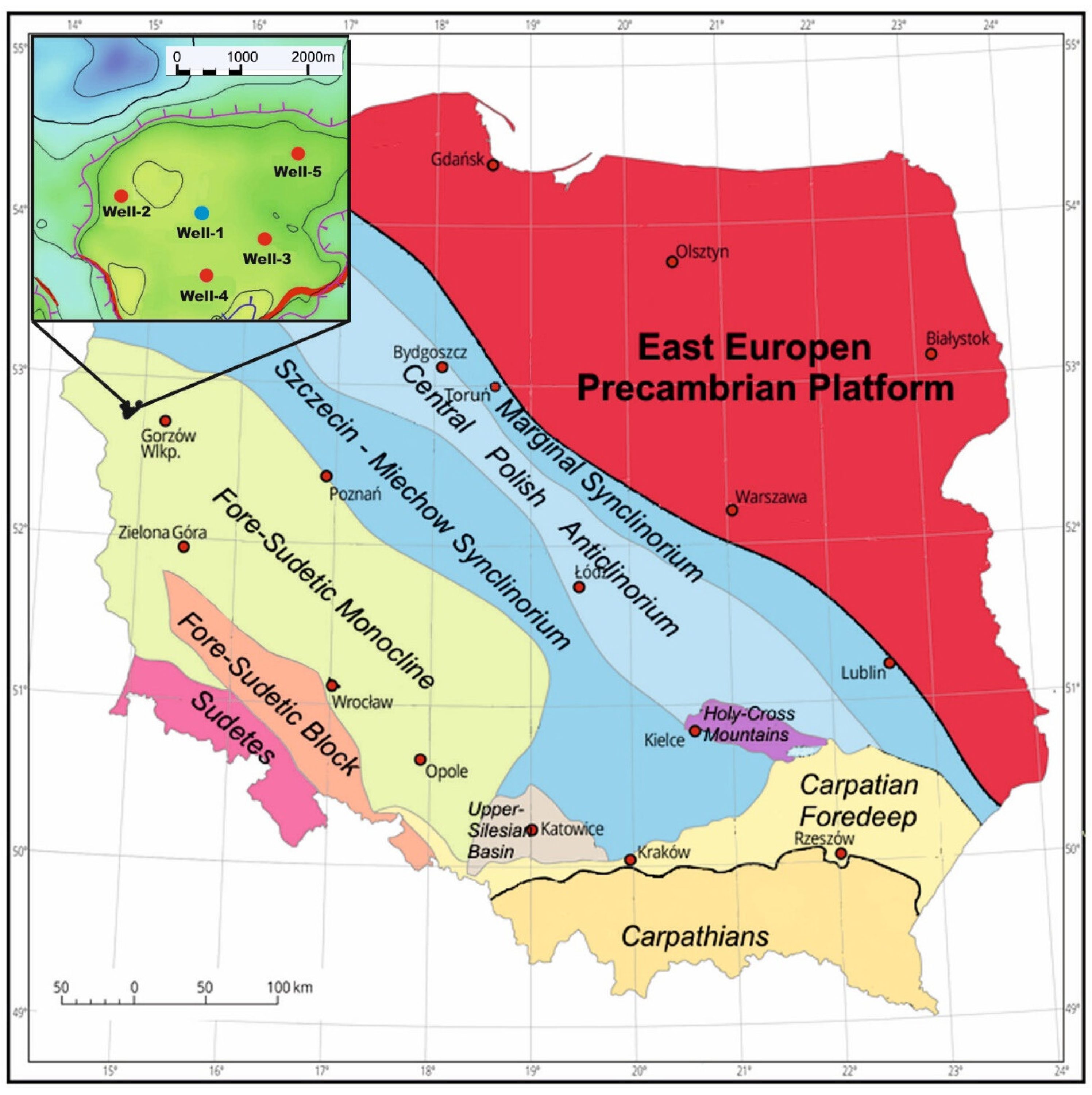
Research and detailed analyses were carried out for a selected area with five wells at one of the largest hydrocarbon reservoirs in the Main Dolomite in the Fore-Sudetic Monocline (Figure 1) in Poland [24]. The Barnówko-Mostno-Buszewo (BMB) reservoir, from which the data are derived, was discovered in the early 1990s [25,26]. More than 40 wells have been drilled in the field to date.
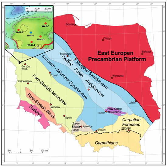
Figure 1.
Map of Poland with a marked area of study. Well-1, marked on the map with a blue dot, is the target of our research (after [24]—modified).
This oil and gas reservoir has been discovered, such as barriers forming the edge zones of the Zechstein carbonate platforms, where increased porosity allows the accumulation of hydrocarbons. Good reservoir properties result from intergranular porosity and fractures observed in the dipmeter log [27,28]. The thickness of the Main Dolomite ranges from 21 to 36 m here, and it is situated on the anhydrite formations (A1G). From the top, directly on Ca2, there are anhydrite (A2) deposits with a thickness of 5 to 9 m. Then there are evaporative deposits of cyclothems: Stassfurt (Z2), Leine (Z3) and Aller (Z4) with a total thickness of more than 400 m. The considerable thickness of the salt-anhydrite formations is responsible for the Groningen effect in the low-resistivity parts of the Main Dolomite.
A set of five wells from Well-1 to Well-5 was selected on the reservoir, for which the data presented in Table 1 were collected. For all wells the following measurements are available: natural gamma-ray GR (API), shallow resistivity LLS (ohmm), deep resistivity LLD (ohmm), sonic compressional slowness DT (us/m), caliper CALI (mm), bulk density RHOB (g/cm3), neutron porosity NPHI (%). The deep resistivity Groningen corrected measurement, LLDO (ohmm), is also available for four out of five wells. The LLD resistivity measurement with Groningen correction was not performed at Well-1, which is situated in the centre of this area, between the other wells. The LLDO curve in the considered boreholes can be taken as the Rt curve. The main goals were to create and evaluate electrofacies and predict the LLDO (Rt) value in Well-1.

Table 1.
Well log data available to electrofacies analysis.
Figure 2 shows an exemplary visualisation of the logs from Table 1 for Well-1 and Well-4. Figure 2a shows the measurements from Well-4, which has been qualified as the reference well for EF calculation and training neural networks. Figure 2b shows the measurements from Well-1, where no LLDO measurement with Groningen correction was performed. In this well, the RT_PRED (LLDO prediction) curve will be predicted based on EF and neural networks models.
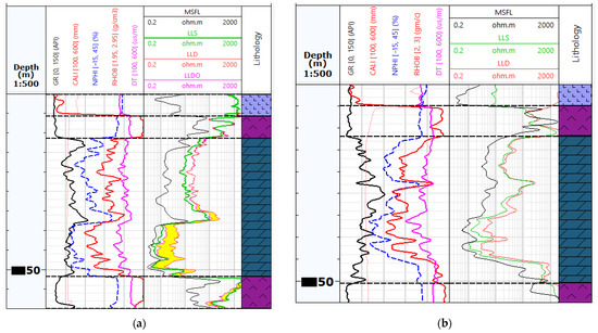
Figure 2.
An example of well-logging data in the analysed wells: (a) An example of Well-4 with a complete set of data, the yellow colour marks the difference between the LLD measurement (overestimated due to the Groningen effect) and the LLDO measurement, which corresponds to the true resistivity value Rt; (b) Summary of measurements in Well-1, without the LLDO measurement.
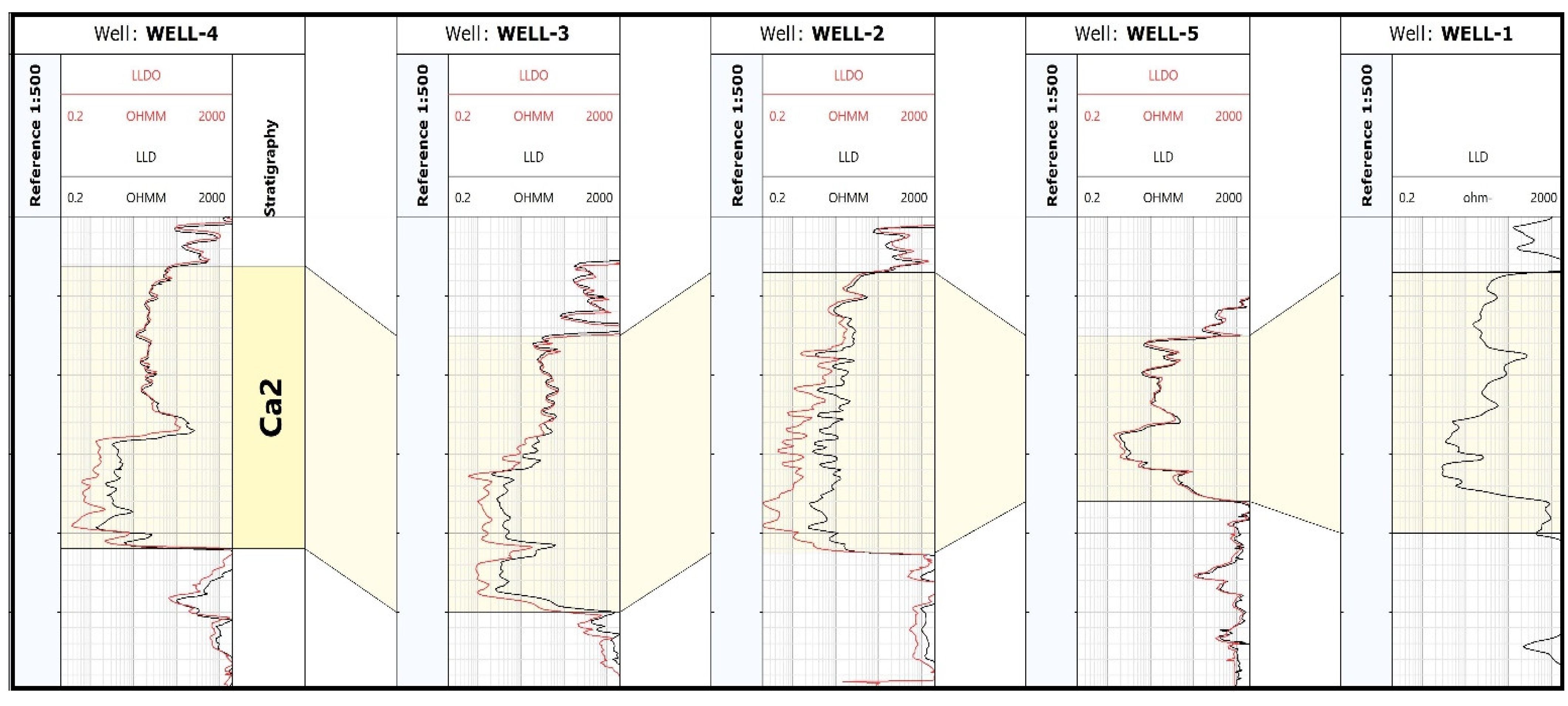
Figure 3 summarises the distribution of resistivity from the deep laterologs LLD and LLDO. In Well-4, the duality of the Main Dolomite (Ca2) interval is particularly visible, related to different reservoir parameters, mainly with different saturations of water and hydrocarbons. The least visible difference is in Well-5. After comparing the measurement of deep laterolog resistivity (LLD) with the measurement taking into account the Groningen effect (LLDO), the most remarkable differences in resistivity can be seen in the bottom of the Ca2 intervals of Well-2, Well-3, and Well-4. This effect was not recorded in Well-5, while it was not available in Well-1. Due to the most significant differentiation of the resistivity (distinct duality) of Ca2 in Well-4, this well was chosen as the teaching well for further analysis, both when determining electrofacies and during Rt prediction in Well-1.
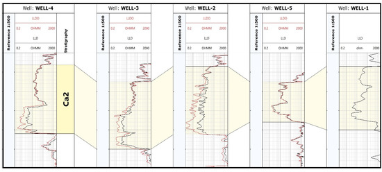
Figure 3.
Combination of LLD and LLDO in the Ca2 interval.
2.1. Electrofacies Calculation
Before building a neural network, a cluster analysis is worth performing to check the heterogeneity of the Main Dolomite. It was known from the available geological data that the Main Dolomite in the studied area might be saturated with gas, crude oil, and formation water. At least two electrofacies with significant water saturation Sw in the bottom part and hydrocarbon saturation Sh in the top part of the Main Dolomite were determined [29,30]. Unfortunately, a reliable Rt is needed to determine the saturation correctly. In four of the five wells, available Rt values were obtained from additional resistivity measurements correcting for the negative impact of the Groningen effect. For detailed analysis, the Geolog Facimage (Emerson Paradigm Holding LLC) [31] program was used, which has several built-in models based on various methods of statistical analysis:
- –
- cluster analysis—Multi-Resolution Graph-Based Clustering (MRGBC) [32], Self-Organizing Map (SOM), Dynamic Clustering, Ascendant Hierarchical Clustering (AHC);
- –
- similarity—Similarity Threshold Method (STM);
- –
- neural networks—Artificial Neural Networks (ANN) [33]. The workflow in the Facimage program it is presented in Figure 4.
 Figure 4. Workflow in the Facimage program to identify facies (based on Geolog, Facimage manual) [34].
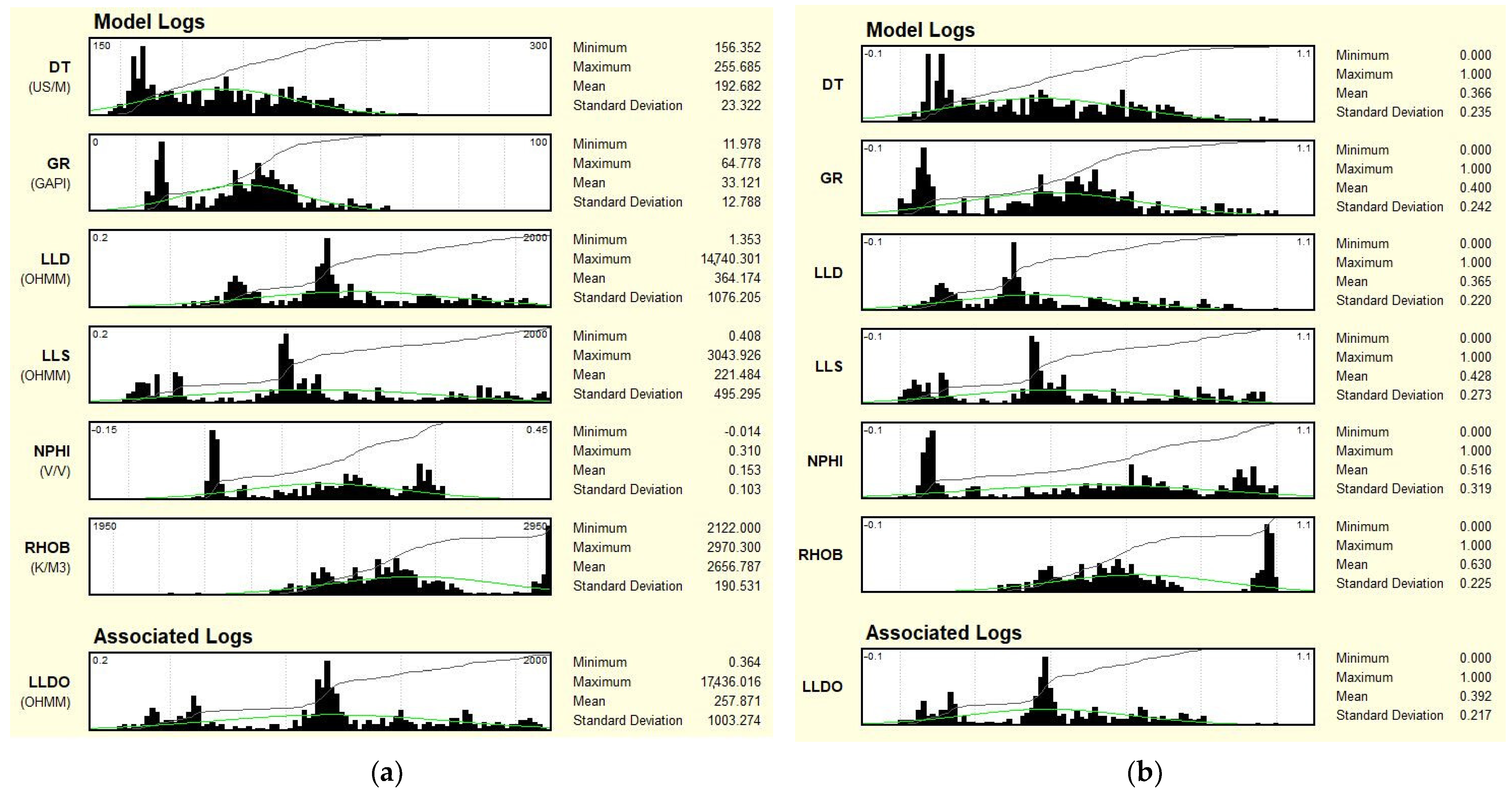
Figure 5 shows the histograms of the well logs from Well-4 that were used to build the model. Figure 5a presents histograms of field data, while Figure 5b shows histograms of normalised logs to release electrofacies. Facies propagation can be performed using two methods: Barycenter or k-NN (k-nearest neighbours).
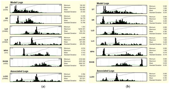
Figure 5.
Histograms of well log data used in MRGBC model: (a) Measurement’s data presented in scales in which they were recorded; (b) After normalisation to calculate electrofacies.
Another module used to build the electrofacies distribution was IPSOM, available in the Techlog, Schlumberger software (AGH University of Science and Technology license), based on Kohonen networks, one of the basic types of self-organising neural networks [35]. A Self-Organizing Map (SOM) differs from typical ANNs both in its architecture and algorithmic properties. Its structure comprises a single-layer linear 2D grid of neurons. All the nodes on this grid are connected directly to the input vector but not to one another, meaning the nodes do not know the values of their neighbours and only update the weight of their connections as a function of the given inputs. The grid is the map that organises itself at each iteration as a function of the input data.
2.2. True Resistivity Prediction (Rt_PRED/LLDO_PRED)
Logs in the Facimage program can be predicted in four ways using k-NN and Barycenter in clustering models and using the ANN or regressions log prediction method. In ANN, it is possible to select the number of epochs (minimum 300) and the number of hidden layers (minimum 2).
Alternatively, the possibility of applying artificial neural networks for LLDO (Rt) prediction was checked using the PS IMAGO PRO (ver. 7) programme based on the IBM SPSS Statistics (ver. 27) analytical engine [36]. IBM SPSS Statistics is a well-known statistical software widely used for statistical analysis and data mining. It also has a Neural Networks module for multilayer perception (MLP) model building. The resistivity logs (LLD, LLS, and LLDO) were logarithmised to reduce the skewness of distributions. Three models were built: one on each of the data sets from Well-2, Well-4, and Well-5, and additionally a fourth model in which the predicted value of the target variable was calculated as the arithmetic mean of the values obtained from the three models mentioned above. In each model, the target variable was LLDO (Rt), and the predictors were LLD, LLS, GR, DT, RHOB, and NPHI. In the beginning, the grouping of observations was performed using the two-step cluster analysis (2SC) method [37,38]. This method was designed to handle very large datasets with both continuous and categorical variables. It has two steps. First, cluster the cases into many small sub-groups using the so-called cluster feature tree. Second, cluster the sub-groups resulting from the pre-cluster step into the desired number of groups using hierarchical clustering. 2SC can also automatically select the optimal number of clusters based on Schwarz’s Bayesian Information Criterion (BIC). Assignment to the clusters designated in this way was then used as one of the predictors in the constructed MLP models.
The quantitative variables introduced into the model of artificial neural networks MLP were standardised. In IBM SPSS Statistics, the MLP models have an input layer, one or two hidden layers, and an output layer. The number of neurons (excluding the bias unit) in the input layer equals the sum of the number of all quantitative predictors and the number of qualitative predictor categories. The number of neurons in two hidden layers was chosen automatically. The output layer has one neuron for the quantitative target variable. Each neuron from a given layer is connected to all neurons from the next layer. Connections have assigned weights, which are initially numbers in the range [0; 1]. As an output from each neuron of the hidden and output layers, we obtain the value of the activation function on the linear combination of input signals and weights. The activation function for the hidden layers was a hyperbolic tangent and for the output layer—identity. The weights are corrected in the learning process by the backpropagation algorithm so that the error function defined as the sum of the squared errors reaches a minimum. The number of epochs in this learning process was set as 1000. To avoid reaching the local minimum instead of the global one, the learning process was repeated 10 times and the model with the smallest error on the training set was selected.
The quality of the models was verified on the test set containing data from Well-3 restricted to the Main Dolomite. The point of reference for all models was the LLDO approximation by the LLD. The values of the root mean squared error and the absolute error were compared. The root mean squared error (RMSE) for the target variable is defined using Formula (1)
and the mean absolute error (MAE) is defined using Formula (2)
where: denotes the observed and denotes the predicted value of the target variable for the i-th observation [39].
3. Results
3.1. Electrofacies Calculation
After performing the calculations with all available methods in the Facimage program, it was decided to present the results obtained with the MRGBC model, as they were the best. This method is quite commonly used in the analysis of well logs data [40,41]. As a result of the cluster analysis using the MRGBC method, six electrofacies were separated in Well-4 and propagated to the remaining wells in the considered depth intervals. The statistical characteristics of individual EF calculated in Well-4 are presented in Figure 6. Facies_1 corresponds to salt formations, Facies_2 corresponds to anhydrite formations, while Facies_3 to 6 correspond to Main Dolomites with different reservoir parameters. The best reservoir parameters of the formation can be observed on Facies_5 and 6, which is related to porosity.

Figure 6.
Electrofacies calculated in Well-4.
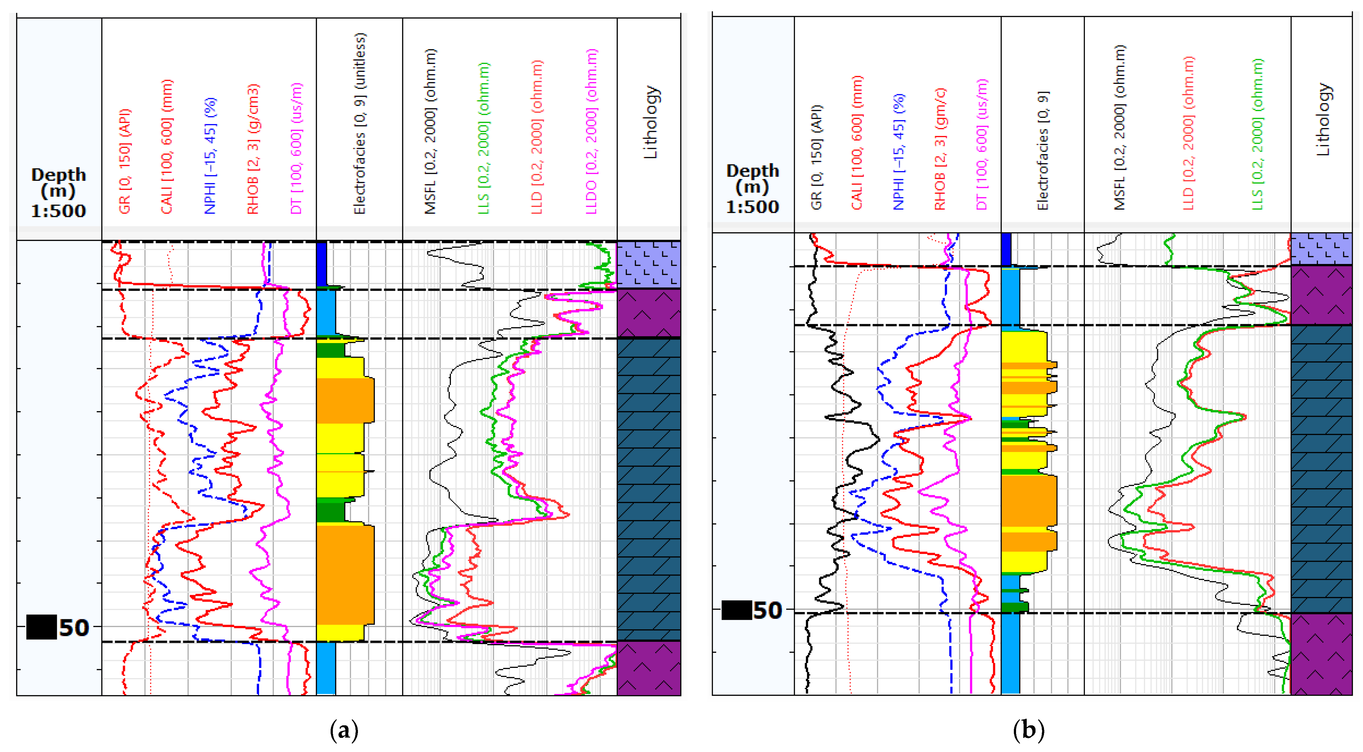
At the histograms of individual facies (Facies_1 to 6) and measurement curves, presented in Figure 6, it can be seen that the DT curve had a minimal effect on the facies division, and it could well be omitted in the cluster analysis. The results of the model’s operation are presented in Figure 7a—the analysis of electrofacies at Well-4, and Figure 7b—the effects of the propagation of the model built on Well-4 over Well-1. In this case, the k-NN (k-nearest neighbours) as a facies propagation method was used.

Figure 7.
An example of well logging data and electrofacies calculation: (a) On Well-4 with a complete set of data, (b) Summary of measurements and electrofacies calculation in the Well-1, using the MRGBC model built on Well-4.
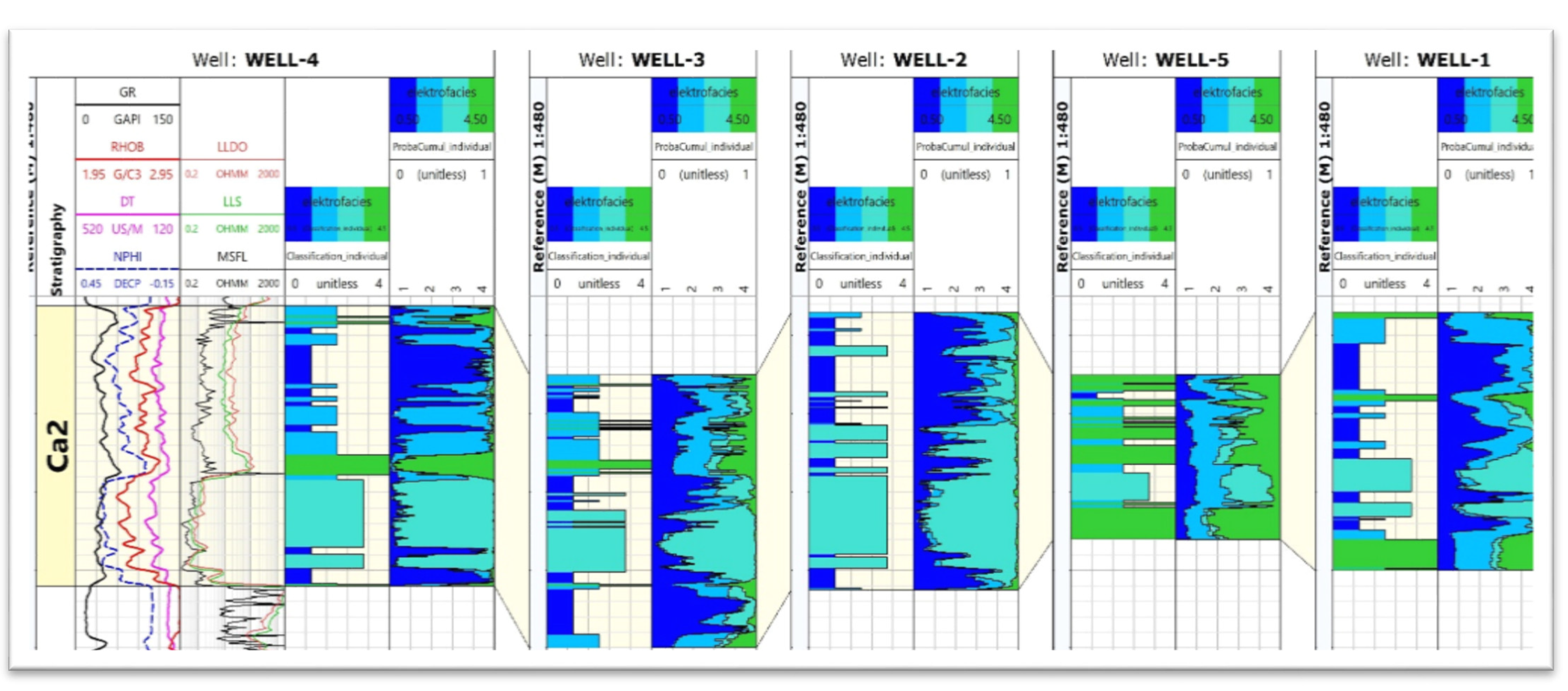
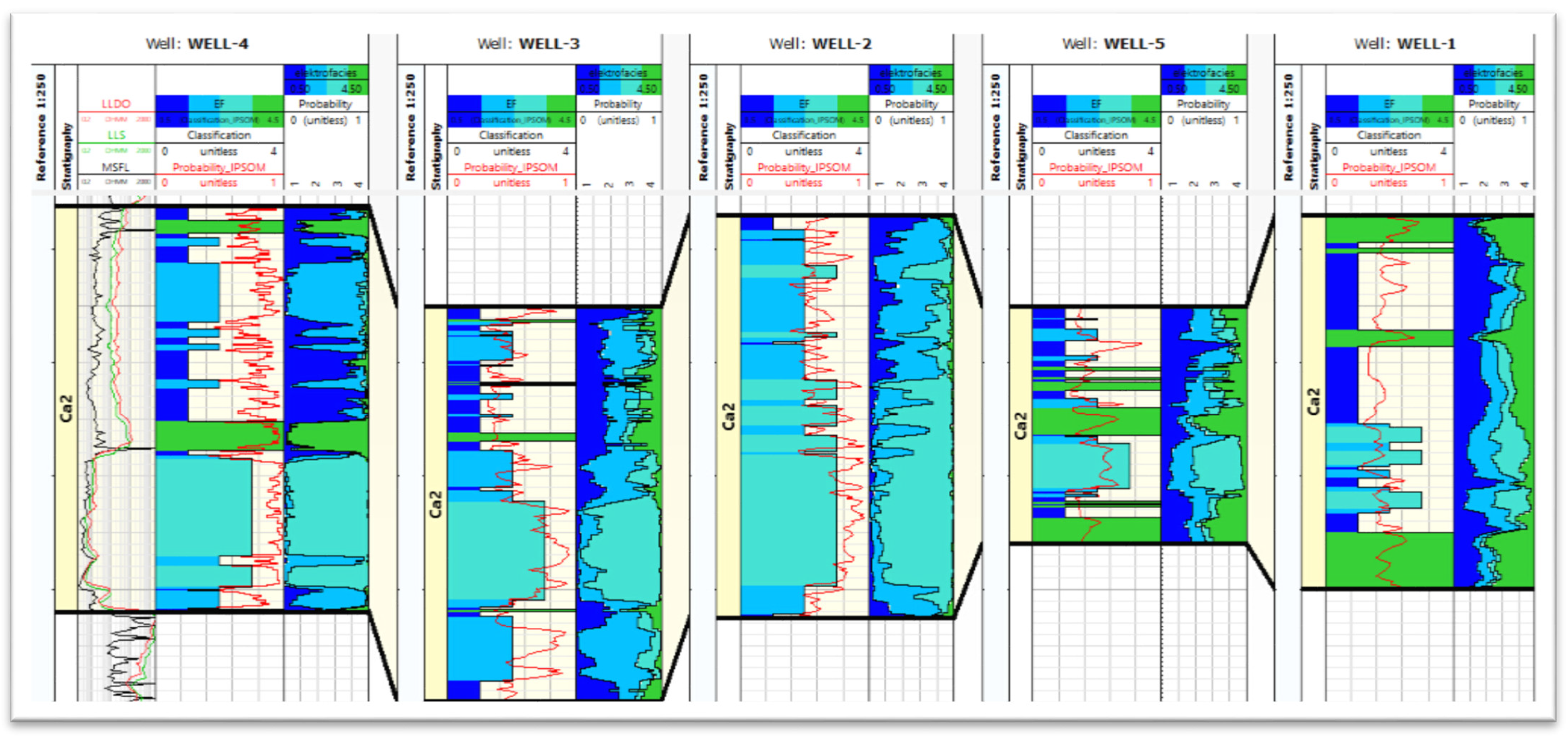
Figure 8 and Figure 9 show the results of the Kohonen network application (IPSOM, Techlog software, Schlumberger, Houston, TX, USA) for the determination of EF in the analysed wells. The analysis was performed for the Main Dolomite interval twice. In the first stage, in each well, the EF were determined individually (Figure 8). In the second stage, the Kohonen network was taught to recognise electrofacies only in Well-4. Subsequently, the constructed network was applied to predict EF in the remaining four wells (Figure 9). Divisions into different numbers of groups were tested. The best result was obtained for four groups. Furthermore, statistical analysis showed the probable presence of four groups. As a result, for both cases, it was decided to separate the four groups.

Figure 8.
Results of electrofacies determination using the IPSOM module, each well was learned individually. The following paths are summarised: DT, GR, RHOB and NPHI input logs (only for Well-4), LLDO, LLS, MSFL resistivity logs (in the Well-1 only LLS and MSFL, no LLDO) (only for Well-4), separated electrofacies, distinguished by colour, determined for the Ca2 interval, for each well individually, and probability curves of a given electrofacies (the one for which the probability of occurrence is the highest—“winning facies” is selected).

Figure 9.
Results of electrofacies determination using IPSOM module, the network was learned only for Well-4, results of learning were applied to other wells. The following paths are summarised: LLDO, LLS, MSFL resistivity logs (in the Well-1 only LLS and MSFL, no LLDO) (only for Well-4), separated electrofacies, distinguished by colour, determined for the Ca2 interval, learned in Well-4 and after that applied to other wells probability function—on a scale from 0 to 1 [unitless] shows the probability of a correct choice of facies, probability curves of a given electrofacies (the one for which the probability of occurrence is the highest—“winning facies” is selected).
As it can be seen, in the first stage, when electrofacies were determined individually for each well (Figure 8), all four facies were distinguished in Well-4. Facies 1 (dark blue) and 2 (medium blue) dominate in the top part, while facies 3 (light blue) and 4 (green) dominate in the bottom part. A similar situation can be seen in Well-3. Alternating facies 1 and 3 were observed in Well-2, while facies 4 dominates in Well-5, with the present interfaces of facies 2 and 3. In Well-1, alternating facies 1, 2, 3, and 4 were observed.
In the second stage (Figure 9), electrofacies were determined for a network learned only on Well-4 data. The network was then applied to determine EF in the remaining wells. In these wells, similar results were obtained as in the first stage. The highest differences were recorded in Well-2, where in the second stage, mostly facies 2 and 3 were observed. This result means that Well-4 is a representative well including all cases occurring in the analysed group, and the network learned only on this well can be successfully used to predict EF in the remaining wells.
Based on a comparison of the average values of the input logs in individual groups, the selected electrofacies were characterised:
- –
- electrofacies 1 (dark blue)—characterised by the lowest GR logs indication (average 13 API), average bulk density of 2.59 g/cc, average transit interval time 60 us/ft, and average neutron porosity on the order of 20%. It is characterised by high deep resistivity (10 ohmm) and a large filtration zone;
- –
- electrofacies 2 (medium blue)—characterised by relatively (in comparison to other groups) high GR logs indication (average 20 API), average bulk density of 2.62 g/cc, average transit interval time 57 us/ft, and medium average neutron porosity on the order of 15%. It is characterised by high deep resistivity (14 ohmm) and a large filtration zone;
- –
- electrofacies 3 (light blue)—characterised by low GR logs indication (average 14 API), the lowest average bulk density of 2.44 g/cc, average transit interval time 68 us/ft, and highest average neutron porosity on the order of 28%. It is characterised by relatively (in comparison to other groups) low deep resistivity (4 ohmm);
- –
- electrofacies 4 (green)—characterised by the highest GR logs indication (average 23 API), the highest average bulk density of 2.70 g/cc, the lowest average transit interval time 52 us/ft, and the lowest average neutron porosity on the order of 7%. It is characterised by high deep resistivity (17 ohmm) and a large filtration zone.
3.2. True Resistivity Prediction (Rt_PRED/LLDO_PRED)
The prediction of the Rt curve was performed using ANN in Facimage and MLP in the IBM SPSS Statistics. The ANN tests in Facimage were performed for various epochs and hidden layers, but increasing epochs and hidden layers did not significantly improve the results. Eventually, the results were obtained with the parameters of 500 epochs and three hidden layers. Figure 10 shows the well log data and RT_PRED prediction results from Facimage learned in Well-4.
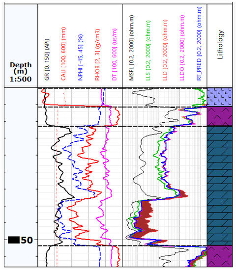
Figure 10.
Well logging data and RT_PRED from Well-4. The brown colour shows the difference in the LLD value from the measurement and the RT_PRED value from the prediction.
The brown colour shows the difference in the LLD value from the measurement and the RT_PRED value from the prediction. As can be seen, the LLD value in the bottom part was reduced similarly to the LLDO measurement (Figure 2a). The difference between LLDO and predicted RT_PRED from ANN learning is very convergent.
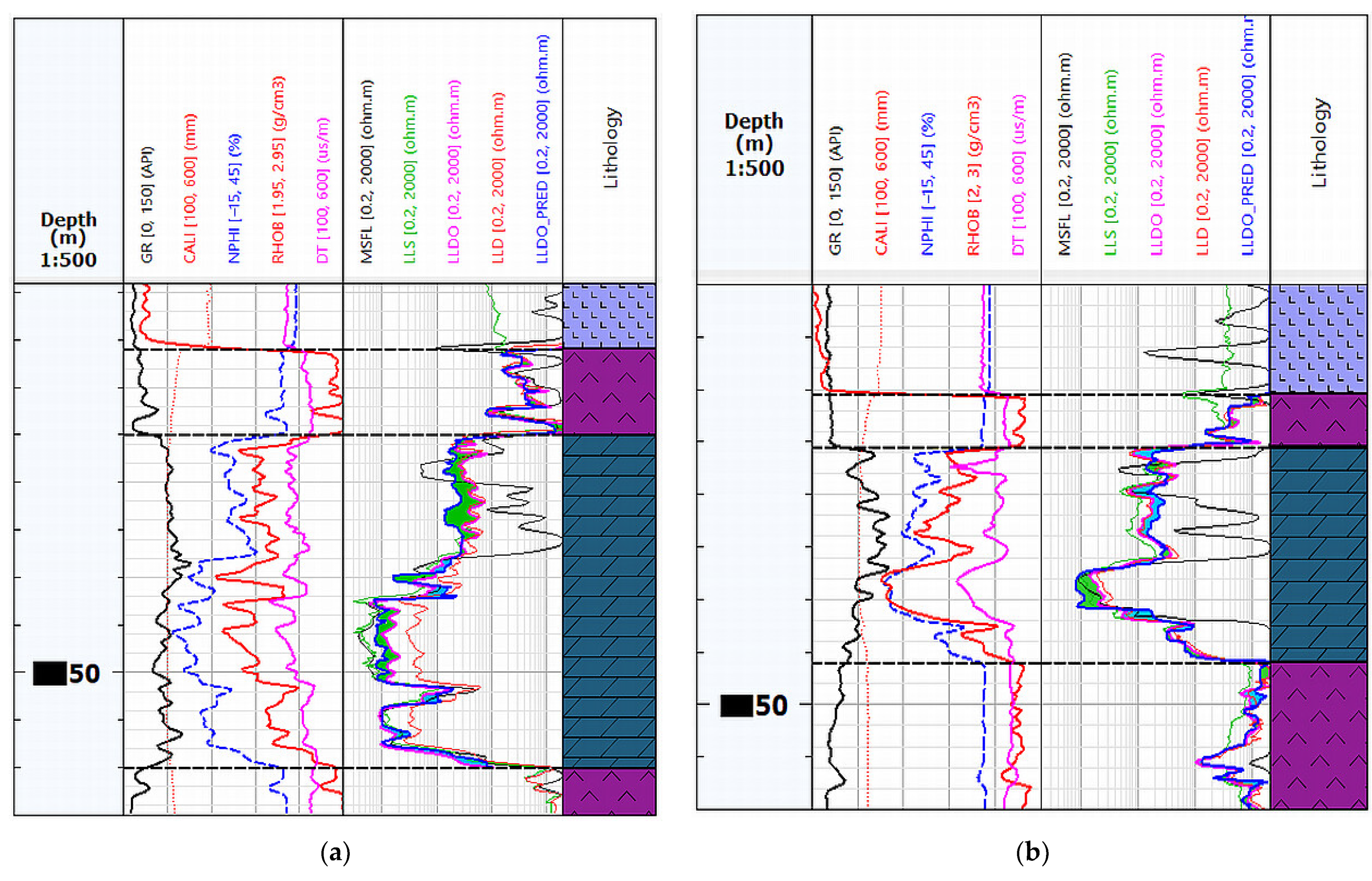
Then the model built on Well-4 was tested on Well-3 and Well-5. The model implementation results on Well-3 and Well-5 are presented in Figure 11a,b, respectively. As can be seen in Figure 11a,b, the differences between the measured values of LLDO and the values LLDO_PRED from the prediction of the neural network learned on Well-4 are very similar and can be used in the further interpretation of saturation.
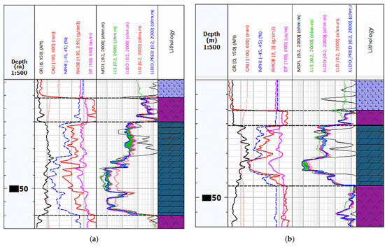
Figure 11.
Summary of well logging data in the tested wells, the RT_PRED values below the LLDO are marked in green and above the LLDO in blue: (a) Well log data from Well-3 with Rt prediction (LLDO_PRED); (b) Well log data from Well-5 with Rt prediction (LLDO_PRED).
Various models of multilayer perceptrons were also examined in IBM SPSS Statistics. They were built on Well-2, Well-4, and Well-5 and tested on Well-3. The prediction quality was checked for models with original LLS, LLD, and LLDO resistivity values and models with logarithmised LLS, LLD, and LLDO values. Additionally, it was checked if adding the grouping step before building the multilayer perceptron model would improve the prediction quality. Indeed, it turned out that the diversity of the geological structure was reflected in the results of 2SC. Three good quality clusters were obtained corresponding to the main dolomite, salt, and anhydrite deposits. The variable identifying membership of these clusters was then introduced as a predictor of the MLP model, significantly improving its quality. Furthermore, a much better quality of prediction characterised models built based on logarithmic values of resistivity. To take advantage of the natural location of Well-1 between Well-2, Well-4, and Well-5 wells, a model was also built that averaged the values predicted by MLP on individual wells. As could be expected, this model turned out to be better than the previous ones. Table 2 summarises RMSE and MAE values for log(LLDO) and LLDO prediction by LLD and best models tested on Well-3.

Table 2.
RMSE and MAE values for log(LLDO) and LLDO prediction by LLD and various models tested on Well-3.
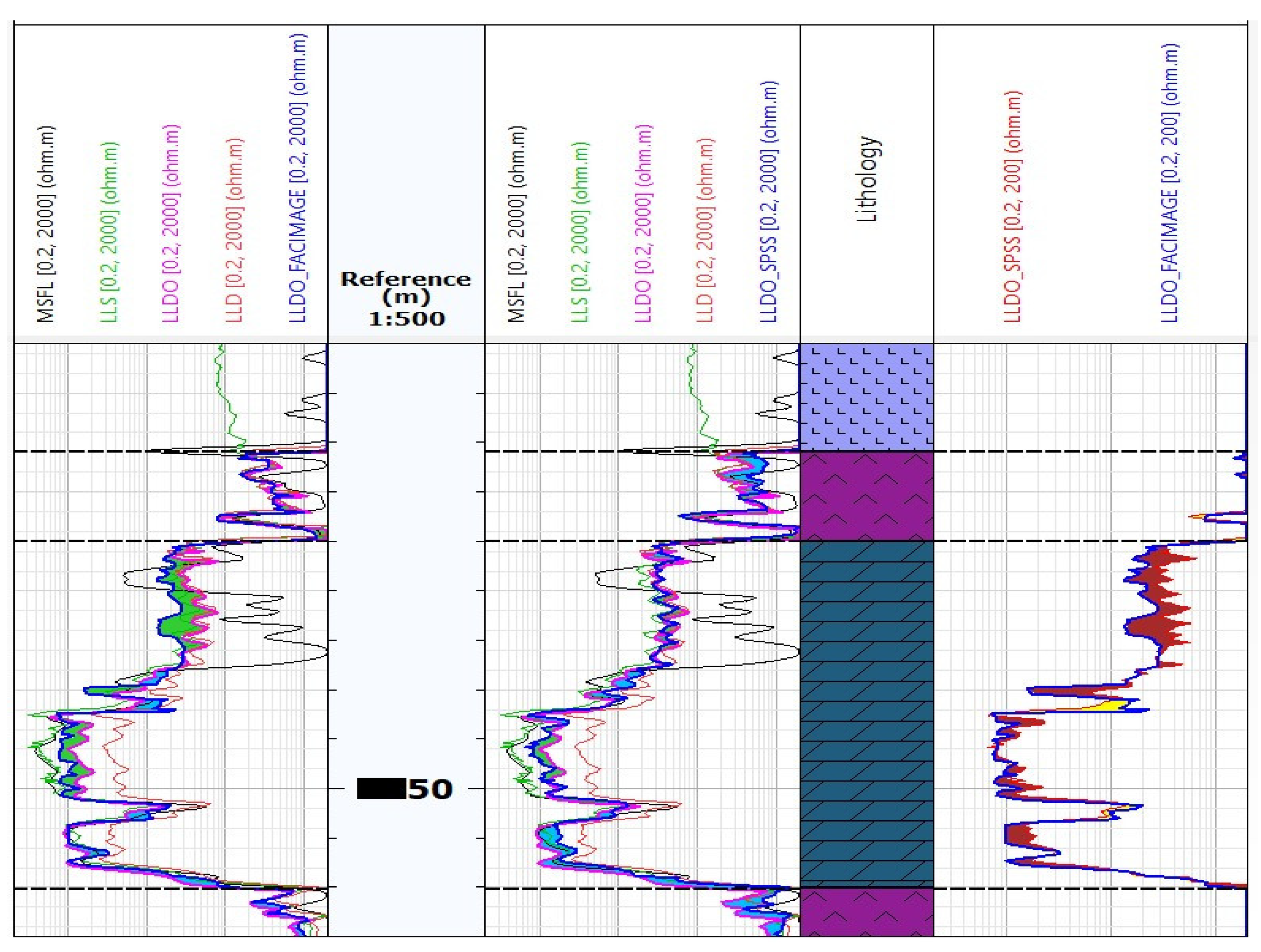
Based on Table 2, it can be observed that the network built in Facimage on Well-4 gives the smallest MAE(LLDO) = 9.3463 error. On the other hand, if we consider logarithmised data, the smallest MAE(log(LLDO)) = 0.1837 error gives the model defined as the mean value of the values predicted by networks built on Well-2, 4, and 5 in IBM SPSS Statistics program. Figure 12 shows the result of LLDO (Rt) prediction by these two models on Well-3. Tracks 1 and 2 compile the resistivity logs and LLDO_PRED curves from the Facimage and the IBM SPSS Statistics predictions, respectively. On track 3, the two prediction curves on a smaller scale from 0 to 200 ohmm have been compiled to refine the differences. The prediction of both curves is satisfactory and does not differ significantly from the LLDO measurement curve.
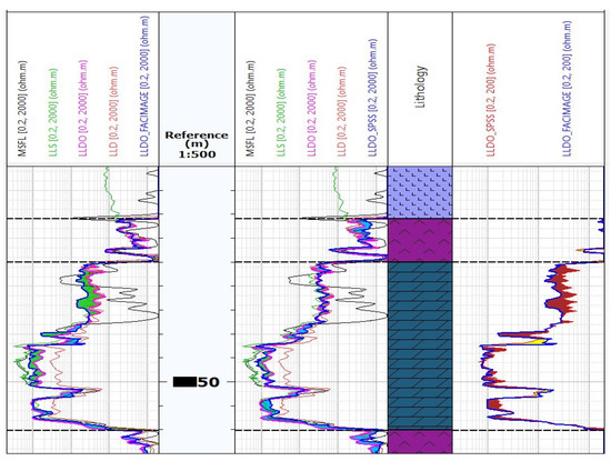
Figure 12.
Comparison of the calculated LLDO_FACIMAGE and LLDO_SPSS resistivity values on Well-3.
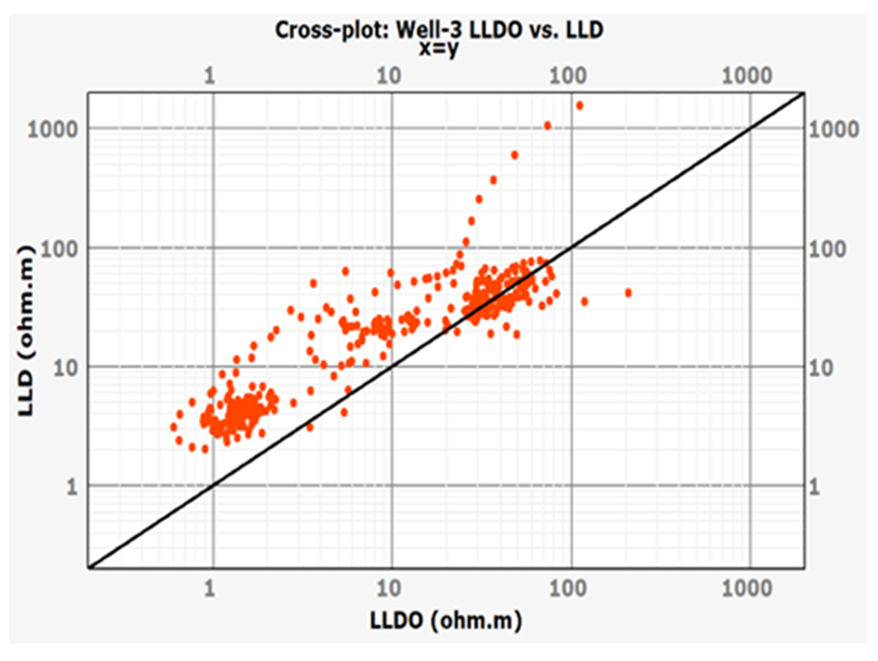
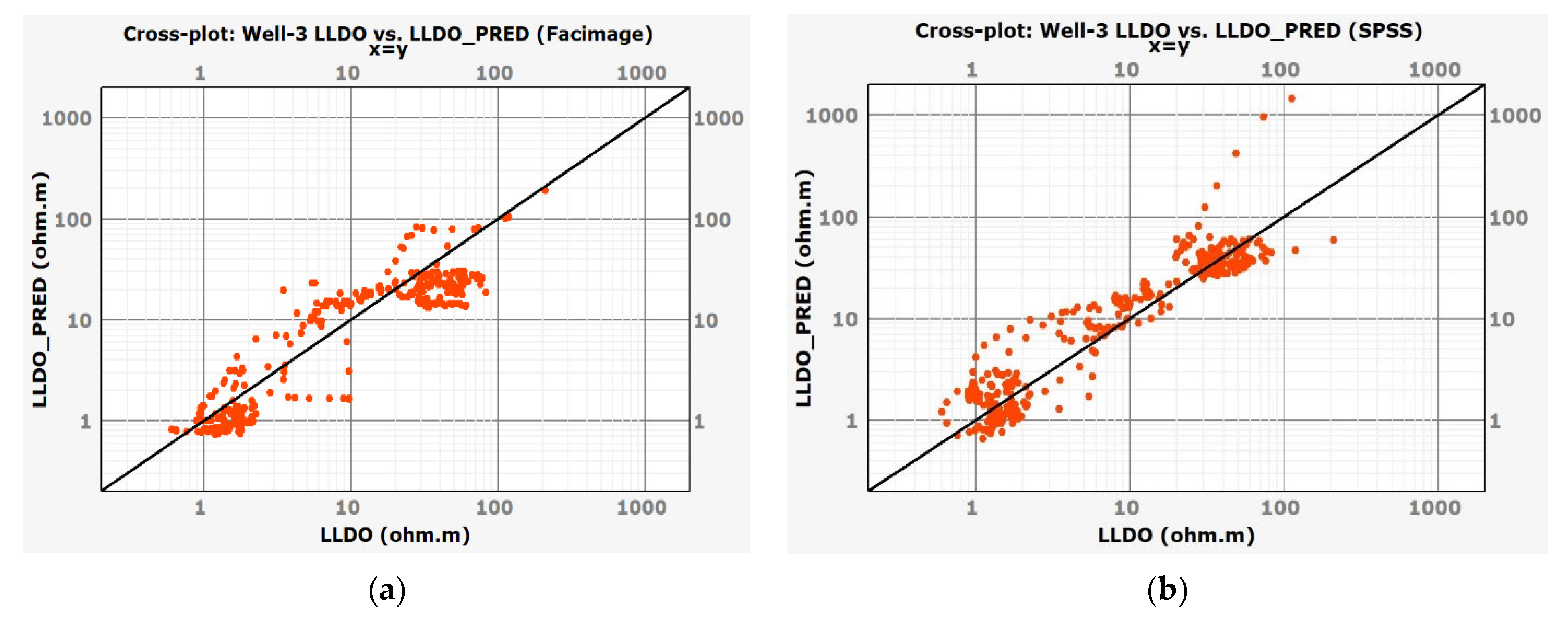
A scatterplot (Figure 13) was made to show the relationship between the measured LLDO value and the deep resistivity log LLD. As can be seen, the LLD overestimates the values of LLDO. Figure 14a,b show the fit of LLDO values predicted by best models built in the Facimage and IBM SPSS Statistics programs to the LLDO measured values. As can be seen, the observations fit line quite well.

Figure 13.
Scatterplot illustrating the prediction of LLDO by LLD on Well-3 with line added.
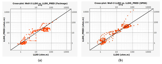
Figure 14.
Scatterplots of predicted values LLDO_PRED from two best models and LLDO measurements on Well-3: (a) LLDO_PRED calculated in the Facimage program based on Well-4 and tested on Well-3; (b) LLDO_PRED calculated in the IBM SPSS Statistics program based on the mean value of three networks (built on Well-2, 4, and 5) and tested on Well-3.
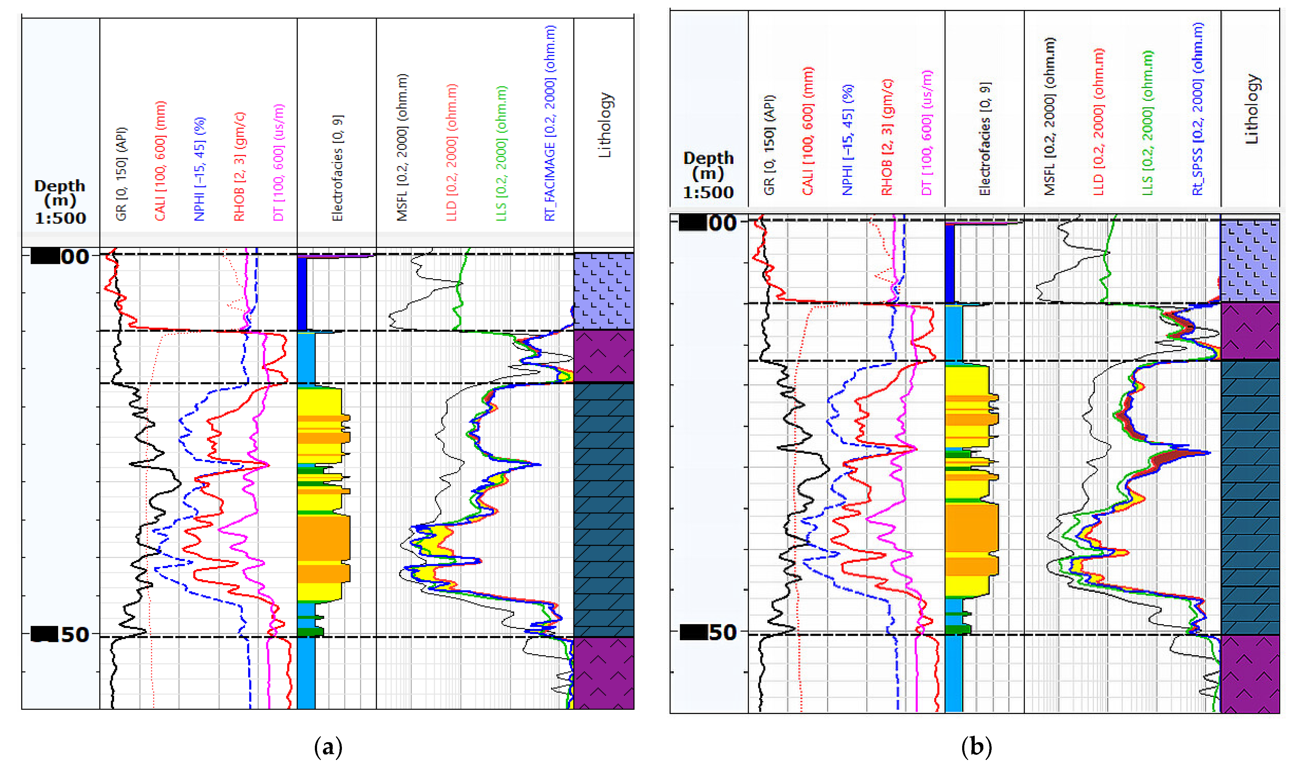
Figure 15a,b show the final results of the models’ prediction on Well-1. They summarise the resistivity measurements, electrofacies is and Rt prediction curves in Facimage and IBM SPSS Statistics programs, respectively.
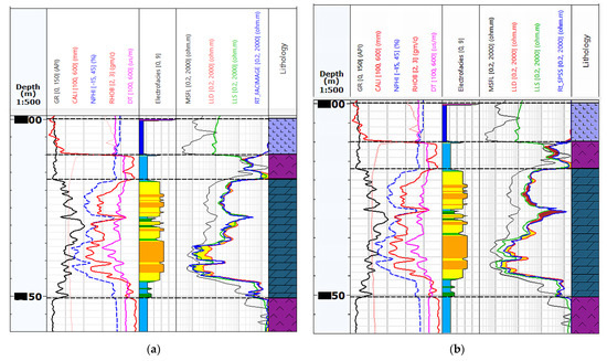
Figure 15.
Comparison of the Rt (blue curve on resistivity track) curve prediction using the Facimage and the IBM SPSS Statistics programs on Well-1. The yellow colour marks the area where the Rt values are below the LLD, and the brown colour marks the area where the Rt values are over the LLD. (a) Well-1 logging data with RT_FACIMAGE predicted in the Facimage program; (b) Well-1 logging data with RT_SPSS predicted in the IBM SPSS Statistics program.
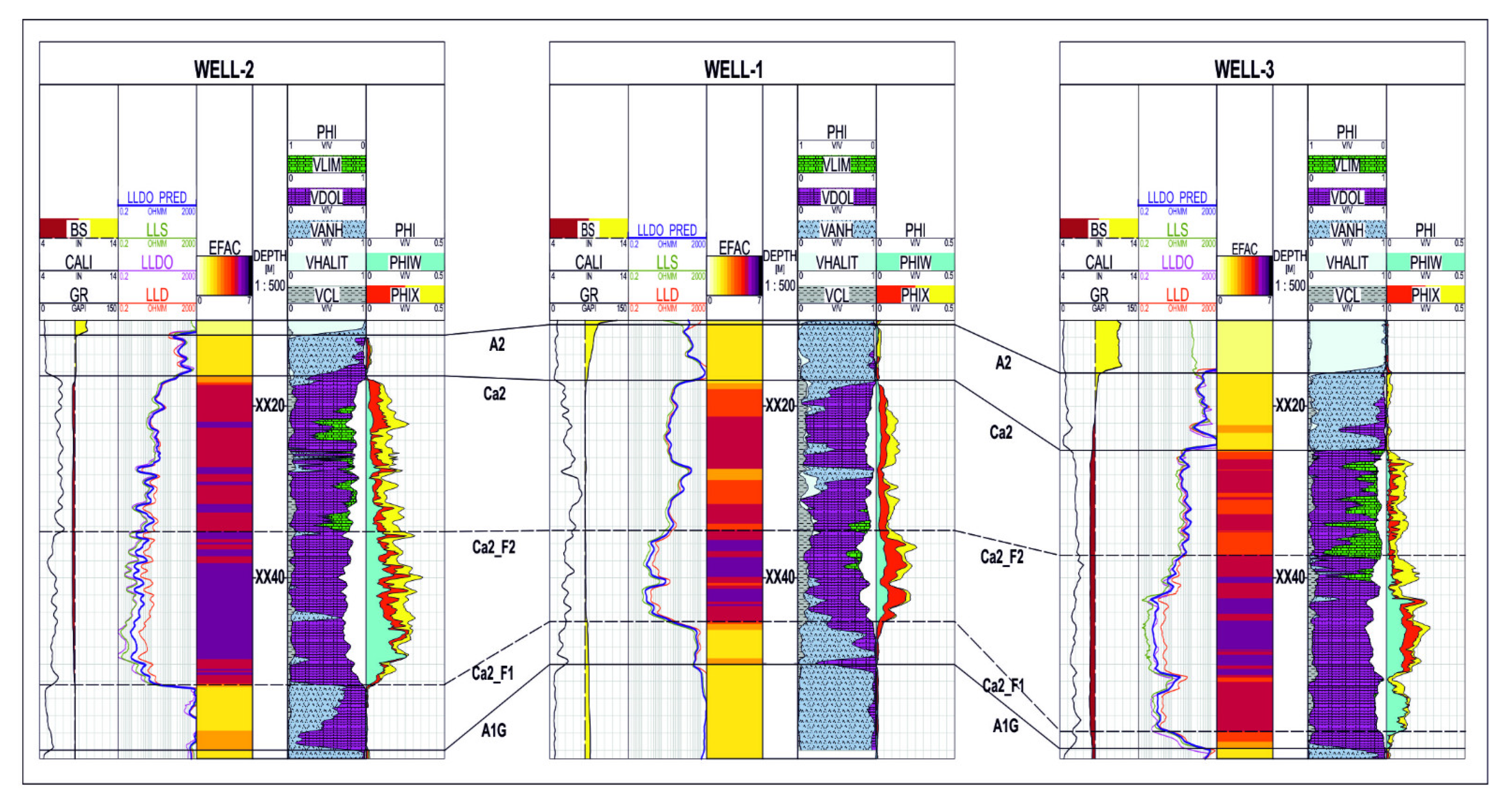
Figure 16 and Figure 17 present the cross-sections combining the determined electrofacies with the available results of the conventional petrophysical interpretation. The lithological solution and the saturation distribution in the analysed wells have been compiled on the last two paths. The results of the interpretation were not taken into account in the EF calculation and analysis. A high correlation of the “dark violet” facies with the bottom interval of the Main Dolomite, characterised by increased porosity, was noticed. The bottom interval is also more water-saturated. Anhydrite intervals below and above the Ca2 interval were clearly separated, but also anhydrite thin beds inside the Ca2 (yellow facies) were noticed. The high correlation of the results of the algorithms used to extract electrofacies with the results of the standard interpretation confirms the legitimacy of using machine learning methods to distinguish the internal differentiation of the Main Dolomite intervals.
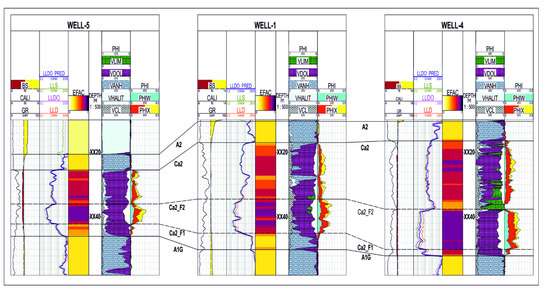
Figure 16.
Cross-section through Well-5, Well-1, and Well-4.
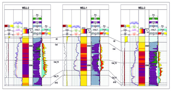
Figure 17.
Cross-section through Well-2, Well-1, and Well-3.
4. Discussion and Conclusions
The research described in the article aimed to find out to what extent recently popular methods, such as data mining, machine learning, neural networks, cluster analysis, can be helpful in the interpretation of well log data. For this purpose, specialised borehole data analysis software (Facimage, Paradigm and Techlog, Schlumberger) and dedicated algorithms (MRGBC, IPSOM), as well as the statistical software (IBM SPSS Statistics), were used. The results of these works are very convergent, which confirms the sense of using statistical analyses in the interpretation of well log data. Nevertheless, it has been noticed that very good results of the Rt curve prediction are obtained if numerous wells with a complete set of measurements are available. Developing an accurate neural network model on a well-known hydrocarbon field can significantly accelerate the assessment of hydrocarbon/water saturation when drilling subsequent production wells on the field.
A large amount of data is the way to succeed because some well’s missing measurements can be completed using modern data analysis methods. In such situations, it should be borne in mind that the generated curve will not fully replace the real measurement but can significantly help in the lithological and saturation interpretation.
Based on the experience from the above analysis, it has been noticed that in the case of having four wells for building ANN, it is crucial to choose an appropriate well that will be relatively similar to the tested one. Well-4, which was applied to teach the network due to its large diversity in data recording, was successfully used to predict the electrofacies distribution in the remaining wells and to predict Rt in the well, where no measurement was made taking into account the Groningen effect. In the case of Well-2, which has a slightly different structure, building a network on it did not give satisfactory results at the test well. Only the choice of Well-4 allowed the construction of a neural network, the propagation of which to the remaining wells gave good effects and thereby obtained satisfactory results in Well-1. A good solution is also the widest possible use of the available data and the construction of a model based on several holes, which averages the predicted values of the target variable.
Of course, carrying out statistical analyses is a much easier process when one has software is dedicated to a given field of science or industry. Examples of such software for geology are the Facimage or the Techlog, Schlumberger software. The built-in algorithms were adapted to the nature of the analysed data. However, it is not impossible to use general statistical analysis and data mining software such as IBM SPSS Statistics. In some cases, such as not measuring all the required curves, this software may offer much more flexibility. Due to the general purpose, however, it requires much more work due to the need to transform the data properly and the time it takes to perform additional analyses or build extra models.
Author Contributions
Conceptualization, S.B., J.K.-P. and E.P.; methodology, J.K.-P., E.P. and S.B.; validation, S.B., E.P. and J.K.-P.; formal analysis, S.B., J.K.-P. and E.P.; resources, S.B.; writing—original draft preparation, S.B.; writing—review and editing, S.B.; visualization, S.B. and E.P.; funding acquisition, S.B. All authors have read and agreed to the published version of the manuscript.
Funding
The article was financially supported from the first edition of the program of the Polish Minister of Science and Higher Education entitled “Implementation Doctorate” no. 30/DW/2017/01/2 of 29 November 2017.
Institutional Review Board Statement
Not applicable.
Informed Consent Statement
Not applicable.
Data Availability Statement
Not applicable.
Acknowledgments
The presented results were obtained as part of the implementation doctorate, carried out by Stanisław Baudzis at the AGH University of Science and Technology in Kraków, at the Faculty of Geology, Geophysics and Environmental Protection. The Authors thank POGC, Warsaw, Poland and Geofizyka Torun S.A. Services for data allowance. AGH—UST software grants for Techlog (Schlumberger). The authors would like to thank the Editors and Reviewers for their constructive suggestions to improve the quality of the article.
Conflicts of Interest
The authors declare no conflict of interest.
References
- Schmitt, P.; Veronez, M.R.; Tognoli, F.M.W.; Todt, V.; Lopes, R.C.; Silva, C.A.U. Electrofacies Modelling and Lithological Classification of Coals and Mud-Bearing Fine-Grained Siliciclastic Rocks Based on Neural Networks. Earth Sci. Res. 2012, 2, 193. [Google Scholar] [CrossRef]
- Serra, O.; Abbott, H.T. The Contribution of Logging Data to Sedimentology and Stratigraphy. Soc. Pet. Eng. J. 1982, 22, 117–131. [Google Scholar] [CrossRef]
- SEG Wiki Dictionary: Electrofacies. Available online: https://wiki.seg.org/wiki/Dictionary:Electrofacies (accessed on 5 August 2021).
- Davis, J.C. Electrofacies in Reservoir Characterization. In Handbook of Mathematical Geosciences; Daya Sagar, B.S., Cheng, Q., Agterberg, F., Eds.; Springer International Publishing: Berlin/Heidelberg, Germany, 2018; pp. 211–223. ISBN 978-3-319-78998-9. [Google Scholar]
- Puskarczyk, E. Artificial Neural Networks as a Tool for Pattern Recognition and Electrofacies Analysis in Polish Palaeozoic Shale Gas Formations. Acta. Geophys. 2019, 67, 1991–2003. [Google Scholar] [CrossRef] [Green Version]
- Puskarczyk, E. Application of Multivariate Statistical Methods and Artificial Neural Network for Facies Analysis from Well Logs Data: An Example of Miocene Deposits. Energies 2020, 13, 1548. [Google Scholar] [CrossRef] [Green Version]
- Singh, S. Permeability Prediction Using Artificial Neural Network (ANN): A Case Study of Uinta Basin. In Proceedings of the SPE Annual Technical Conference and Exhibition, Dallas, TX, USA, 9–12 October 2005. SPE-99286-STU. [Google Scholar]
- Mohaghegh, S.; Balan, B.; Ameri, S. Permeability Determination From Well Log Data. SPE Form. Eval. 1997, 12, 170–174. [Google Scholar] [CrossRef]
- Huang, Z.; Shimeld, J.; Williamson, M.; Katsube, J. Permeability Prediction with Artificial Neural Network Modeling in the Venture Gas Field, Offshore Eastern Canada. Geophysics 1996, 61, 422–436. [Google Scholar] [CrossRef]
- Quadir, A.; Lewis, C.; Rau, R.-J. Generation of Pseudo-Synthetic Seismograms from Gamma-Ray Well Logs of Highly Radioactive Formations. Pure. Appl. Geophys. 2019, 176, 1579–1599. [Google Scholar] [CrossRef]
- Kim, S.; Kim, K.H.; Min, B.; Lim, J.; Lee, K. Generation of Synthetic Density Log Data Using Deep Learning Algorithm at the Golden Field in Alberta, Canada. Geofluids 2020, 2020, 1–26. [Google Scholar] [CrossRef] [Green Version]
- Suau, J.; Grimaldi, P.; Poupon, A.; Souhaite, P. The Dual Laterolog-Rxo Tool. In Proceedings of the Fall Meeting of the Society of Petroleum Engineers of AIME, San Antonio, TX, USA, 8–11 October 1972. SPE-4018-MS. [Google Scholar]
- Trouiller, J.C.; Dubourg, I. A Better Deep Laterolog Compensated for Groningen and Reference Effects. In Proceedings of the SPWLA 35th Annual Logging Symposium, Tulsa, OK, USA, 19–22 June 1994. [Google Scholar]
- Nam, M.J.; Pardo, D.; Torres-Verdín, C. Assessment of Delaware and Groningen Effects on Dual-Laterolog Measurements with a Self-Adaptive Hp Finite-Element Method. Geophysics 2010, 75, F143–F149. [Google Scholar] [CrossRef]
- Andersen, B.I. Modeling and Inversion Methods for the Interpretation of Resistivity Logging Tool Response. Ph.D. Thesis, Delft University of Technology, Delft, The Netherlands, 2001; pp. 149–151. [Google Scholar]
- Drahos, D.; Galsa, A. Modeling Groningen Effect on Deep Laterolog. Geosci. Eng. Vol. 2015, 46, 9–21. [Google Scholar]
- Woodhouse, R. The Laterolog Groningen Phantom Can Cost You Money. In Proceedings of the SPWLA 19th Annual Logging Symposium, El Paso, TX, USA, 13–16 June 1978. [Google Scholar]
- Lacour-Gayet, P. Method and Apparatus for Detecting an Anomaly in a Resistivity Measurement of an Earth Formation. U.S. Patent No. 4,335,35, 1982. [Google Scholar]
- Chemali, R.E.; Dirk, W.C. Method and Apparatus for Measuring Resistivity of an Earth Formation. U.S. Patent No. 4,646,026, 24 February 1987. [Google Scholar]
- Smits, J.W.; Dubourg, I.; Luling, M.G.; Minerbo, G.N.; Koelman, J.M.V.A.; Hoffman, L.J.B.; Lomas, A.T.; Oosten, R.K.V.D.; Schiet, M.J.; Dennis, R.N. Improved Resistivity Interpretation Utilizing a New Array Laterolog Tool and Associated Inversion Processing. In Proceedings of the SPE Annual Technical Conference and Exhibition, New Orleans, LA, USA, 27–30 September 1998. SPE-49328-MS. [Google Scholar]
- Lee, S.H.; Kharghoria, A.; Datta-Gupta, A. Electrofacies Characterization and Permeability Predictions in Complex Reservoirs. SPE Reserv. Eval. Eng. 2002, 5, 237–248. [Google Scholar] [CrossRef]
- Correia, G.G.; Schiozer, D.J. Reservoir Characterization Using Electrofacies Analysis in the Sandstone Reservoir of the Norne Field (Offshore Norway). Pet. Geosci. 2016, 22, 165–176. [Google Scholar] [CrossRef]
- Baudzis, S.; Jarzyna, J.A.; Puskarczyk, E. The Measurement and Interpretation Methodology of Resistivity Logs Affected by the Groningen Effect—A Polish Case Study. Geol. Geophys. Environ. 2020, 46, 35. [Google Scholar] [CrossRef]
- Jarzyna, J.A.; Baudzis, S.; Janowski, M.; Puskarczyk, E. Geothermal Resources Recognition and Characterization on the Basis of Well Logging and Petrophysical Laboratory Data, Polish Case Studies. Energies 2021, 14, 850. [Google Scholar] [CrossRef]
- Gorski, M.; Wojtkowiak, Z.; Radecki, S. Barnowko-Mostno-Buszewo (BMB); the Largest Crude Oil Deposit in Poland. Pet. Geosci. 1999, 5, 5–15. [Google Scholar] [CrossRef]
- Pikulski, L.; Wolnowski, T. Geological Analysis of the Main Dolomite Formations (Ca2) in Western Poland. In Proceedings of the AAPG/EAGE Internetional Research Conference, El Paso, TX, USA, 15 October 2000. [Google Scholar]
- Karnkowski, P. Oil and Gas Deposits in Poland; Geosynoptics Society “GEOS”: Cracow, Poland, 1999; ISBN 83-86695-01-3. [Google Scholar]
- Karnkowski, P.H. Permian Basin as a Main Exploration Target in Poland. Prz. Geol. 2007, 55, 1003–1015. [Google Scholar]
- Górski, M.; Król, E.; Kunicka-Górska, W.; Trela, M.; Urbańska, H. Wydzielanie pułapek węglowodorów w utworach poziomu dolomitu głównego poprzez rozpoznanie zmian litofacjalnych i strukturalnych na podstawie zintegrowanej interpretacji sejsmiki 3D i danych otworowych w rejonie Gorzowa. Prz. Geol. 1999, 47, 1080–1095. [Google Scholar]
- Krogulec, E.; Sawicka, K.; Zabłocki, S.; Falkowska, E. Mineralogy and Permeability of Gas and Oil Dolomite Reservoirs of the Zechstein Main Dolomite Basin in the Lubiatów Deposit (Poland). Energies 2020, 13, 6436. [Google Scholar] [CrossRef]
- Available online: Https://Www.Pdgm.Com/Products/Geolog/Facimage/ (accessed on 6 August 2021).
- Ye, S.-J.; Rabiller, P. A New Tool For Electro-Facies Analysis: Multi-Resolution Graph-Based Clustering. In Proceedings of the SPWLA 41st Annual Logging Symposium, Dallas, TX, USA, 4–7 June 2000. [Google Scholar]
- Aggarwal, C.C. Neural Networks and Deep Learning: A Textbook; Springer: Berlin/Heidelberg, Germany, 2018; ISBN 978-3-319-94463-0. [Google Scholar]
- Facimage Help, Paradigm/Emerson Geolog-Paradigm 20, Bulit in Manual Facimage 2020; Paradigm Ltd.: Brisbane, QLD, Australia, 2020.
- Kohonen, T. The Self-Organizing Map. Proc. IEEE 1990, 78, 1464–1480. [Google Scholar] [CrossRef]
- Available online: https://Www.Ibm.Com/Analytics/Spss-Statistics-Software (accessed on 5 August 2021).
- Zhang, T.; Ramakrishnon, R.; Livny, M. BIRCH:An Efficient Data Clustering Method for Very Large Databases. In Proceedings of the ACM SIGMOD Conference on Management of Data, Montreal, QB, Canada, 1 June 1996; pp. 103–114. [Google Scholar]
- Chiu, T.; Fang, D.; Chen, J.; Wang, Y.; Jeris, C. A Robust and Scalable Clustering Algorithm for Mixed Type Attributes in Large Database Environment. In Proceedings of the Seventh ACM SIGKDD International Conference on Knowledge Discovery and Data Mining—KDD ’01, San Francisco, CA, USA, 26–29 August 2001; pp. 263–268. [Google Scholar]
- Larose, D.T.; Larose, C.D. Discovering Knowledge in Data: An Introduction to Data Mining, 2nd ed.; Wiley: Hoboken, NJ, USA, 2014; ISBN 978-1-118-87357-1. [Google Scholar]
- Tian, Y.; Xu, H.; Zhang, X.-Y.; Wang, H.-J.; Guo, T.-C.; Zhang, L.-J.; Gong, X.-L. Multi-Resolution Graph-Based Clustering Analysis for Lithofacies Identification from Well Log Data: Case Study of Intraplatform Bank Gas Fields, Amu Darya Basin. Appl. Geophys. 2016, 13, 598–607. [Google Scholar] [CrossRef]
- Wu, H.; Wang, C.; Feng, Z.; Yuan, Y.; Wang, H.-F.; Xu, B.-S. Adaptive Multi-Resolution Graph-Based Clustering Algorithm for Electrofacies Analysis. Appl. Geophys. 2020, 17, 13–25. [Google Scholar] [CrossRef]
Publisher’s Note: MDPI stays neutral with regard to jurisdictional claims in published maps and institutional affiliations. |
© 2021 by the authors. Licensee MDPI, Basel, Switzerland. This article is an open access article distributed under the terms and conditions of the Creative Commons Attribution (CC BY) license (https://creativecommons.org/licenses/by/4.0/).

