Abstract
A new linear regression form is derived for a flux observer and a position observer is designed. In general, the observability of the permanent-magnet synchronous motor is lost at zero speed. In this work, the proposed regressor vector contains current derivative terms in both directions (-axis), and it gives the chance for the model-based flux observer to operate at zero speed. When an excitation signal is injected into d and q axes with the proposed flux observer, it helps to satisfy the persistent excitation condition in the low-speed range. Therefore, the sensorless performance of the model-based is improved greatly, even at zero speed. However, it appears with a disturbance term, which depends on the derivative of the d-axis current. Thus, the disturbance does not vanish when an excitation signal is injected. In this work, the disturbance term is also taken care of in constructing an observer. It results in an observer which allows signal injection. Thus, high frequency signal can be injected in the low speed region and turned off when it is unnecessary as the speed increases. This model-based approach utilizes the signal injection directly without recurring to a separate high frequency model. In other words, it provides a seamless transition without switching to the other algorithm. The validity is demonstrated by simulation and experimental results under various load conditions near zero speed.
1. Introduction
As the cost and reliability of the motor drive system are taken into account, a rotor position sensorless control and algorithms are being widely used in AC motor. In particular, an interior permanent-magnet synchronous motor (IPMSM) is used for industrial, traction applications, and home appliances. Because of reluctance torque, they have a higher power density than non-salient and induction motor. The sensorless control for IPMSM has been researched extensively for decades.
The sensorless methods are classified into model-based and saliency-based methods. The model-based method is applied in medium/high-speed range because it depends on the relative magnitudes of -axis EMFs. The flux or back-electromotive force (EMF) is normally used as an estimated variable involving the fundamental excitation. The dynamic model of a IPMSM is more complex than surface-mount PMSM (SPMSM) in the stationary frame. To simplify the model, the extended back-EMF (EEMF) was proposed for IPMSM sensorless control [1,2,3,4,5,6]. The active flux is more conveniently used in IPMSMs since it includes the rotor saliency, as well as the rotor flux [7,8].
To extend the sensorless operation range, the saliency-based method is used in the low-speed range. It is well known that the injection of high frequency signal increases the signal-to-noise ratio, thereby improving low speed performances significantly [9,10,11,12]. In particular, it enables full torque operation at standstill. However, it causes audible noise and is not suitable for the high speed region. In addition, it limits the bandwidth of the current controller, due to the demodulation method.
Some applications require a wide sensorless operation range, such as electric vehicles, washing machines, crane systems, and electric propulsion for aircraft. Practically, it is beneficial to use a signal injection method at low speed and a model-based method in the high speed region. Then, it requires a switching algorithm between the two methods depending on the speed range. If the switching takes place drastically, chattering may occur. It can be prevented by using a speed-dependent hysteresis changeover [13,14,15,16]. Furthermore, it is better to employ a speed-dependent gain for the smooth transition. On the other hand, the Gopinath filter guarantees a smooth transition. The weight changes dynamically depending on speed [17,18]. An adaptive full-order observer with the signal injection method was utilized in [19]. They focused on the seamless transition between model-based and signal injection algorithms. However, the hybrid systems are more complicated because two different estimated algorithms are implemented.
Recently, a unified model-based sensorless method was proposed as a new approach. By allowing additional signal injection, the performance of the model-based sensorless method was significantly improved [20,21]. Applying Newton’s method to the nonlinear optimization problem, these methods directly estimated the rotor position angle and speed. It did not require the demodulation method nor any switching mechanisms. Therefore, they provided seamless transitions between low and medium speeds. However, these observer models are included in the rotor speed information and pure differential operator.
Other candidates of unified model-based sensorless methods estimate the rotor or active flux [22,23,24,25,26,27,28,29]. Unlike back-EMF, the rotor flux maintains its magnitude regardless of the speed, which is a necessary condition to become a unified model-based sensorless method. To estimate the flux, a full-order observer or a low-pass filter was used to deal with unknown initial values and DC offset problems. Since the rotor speed information is included in the model, these methods require a speed adaptation method.
A nonlinear flux observer for SPMSM was proposed and experimentally demonstrated in the stationary frame [23,24,25]. Note that the nonlinear observer is practically advantageous because it does not require speed information. Bobtsov et al. [26,27] extended the flux observer by including an initial parameter estimator. The convergence was proved with the persistence of excitation (PE) condition. However, the use of a pure integrator is a critical weakness. To eliminate the DC offset problem, a new flux estimator was proposed by incorporating the parameter estimator and the flux observer [28]. Later, it extended the work to IPMSM in the context of a regressor [29]. An additional feedback loop was constructed based on an observer of regression form. It allowed the high frequency signal injection to increase the signal-to-noise ratio in the low speed range.
The previous observer based on the linear regression model did not work properly at zero speed, even with the high frequency signal [29]. This is because its regressor vector did not satisfy the PE condition. The injected signal helped only to reduce the magnitude of oscillating angle error. In this paper, a regression model-based flux observer is proposed, which can be operated at standstill. To enhance the low-speed sensorless performance, a new regression model is derived by a modified regressor vector. It is derived from the square of the active flux after applying a high-pass filter. Then, it turns out to be a product form between a known vector and an unknown parameter vector. The gradient algorithm is applied to obtain a flux estimation. Though it is a model-based observer, it can operate at zero speed with signal injection under loaded conditions. At high speed, it turns into a flux observer by simply turning off the high frequency signal. This means that the injection algorithm is carried over to a model-based algorithm seamlessly without an additional gadget. It is more advantageous since the speed information is not required in the observer, and a demodulation is not necessary with the signal injection. Experimentally, the low speed sensorless control performance was demonstrated under the rated load torque.
The remainder of this paper is organized as follows. The dynamic model of an IPMSM is discussed in Section 2. In Section 3, the proposed observer and the new linear regression form are derived. Then, the signal injection strategy in zero speed region is proposed in Section 4. In Section 5, the simulations and experiments are shown.
2. Dynamic Model of a IPMSM
The IPMSM is modeled in the stationary - frame as follows [30]:
where R is the stator coil resistance, is the rotor flux linkage, is current, is voltage in the stationary frame, is the electrical speed, and is the differential operator. Angle is the rotor flux angle, , and , where and are the d- and q-axis inductance. Voltage Equation (1) is expressed equivalently as follows:
where is the stator flux, is the derivation of the stator flux, , as follows:
We have two estimates of based on voltage (2) and current (3). The stator current in the synchronous frame is defined as follows:
where Note that is synchronous axis reference frame quantities. To distinguish between the rotor angle-dependent and non-dependent terms, it is obtained by substituting (4) into (3) as follows:
Substituting (5) into (3) and separating the angle dependent term, the active flux is defined by the following [7,8]:
Differentiating both sides of (6), we obtain from (2) the following:
Note that (6) includes the angle information associated with the rotor magnetic saliency. Thus, makes it possible to estimate the angle based on the rotor saliency.
3. Proposed Flux Observer
3.1. Nonlinear Observer Based on Regression Model
Recently, the flux observer was proposed based on the regression model [29]. The standard linear regression form is as follows:
where and are known vectors and is unknown vector. Note that 2 is the dimension of an unknown vector, which can be extended. The standard gradient estimator is derived as follows:
where is a positive adaptation gain.
The advantages of the regression model are the following:
- It does not include uncertain information, such as rotor speed.
- It is easy to develop an observer using a nonlinear optimizing method, such as a gradient descent method.
- It is exponentially stable when the regressor vector is the PE condition [31].
However, the previous regressor vector was not satisfied at standstill, despite additional signal injection [29]. The motive in this paper is to create a new regression model so that the regressor satisfies the PE condition at zero speed.
3.2. New Linear Regression Form Derivation Processing
Note that . Thus, it follows from (6) that the following holds:
In (10), the following identity is used: . Note that a different identity was used in the previous work [29]. Particularly, the coefficient ‘1’ or ‘2’ of makes a difference in the following linear regression form. Rearranging (10), we have the following:
The filter functions as a differentiator. Therefore, it eliminates the effects of constant terms ultimately. Applying the swapping Lemma [32] and grouping with , the proposed linear regression form is derived as follows:
where
The detailed derivation process is included in Appendix A. It should be noted that and are available, since , are available and R, , are assumed to be known. Note again that is available for all , while is exponentially decaying. It is emphasized here that (14) has a linear regression form perturbed by . Specifically, (14) is a product of known vector by an unknown variable, .
3.3. Adaptation Law Using Gradient Algorithm
To derive an observer, gradient rule is applied to regression model (14). Note that the model has two perturbation terms, and . Since decays exponentially, it can be neglected. Note, however, that cannot be neglected during the transient state or when an excitation signal is injected into the d-axis. Previously, it was ignored by assuming that is constant [29].
Usually, signal injection is exercised in the d-axis since it does not cause torque ripple, and gives a minor effect on torque. Typically, the d-axis current is supposed to be with a signal injection strategy, where is a high frequency term. In such a case, cannot be neglected any time.
Considering (6), it is seen that . Therefore, d can be estimated, using a flux estimate, such that the following holds:
Using , a cost function is defined as follows:
Then, the gradient is equal to the following: , where
and is the identity matrix.
Combining with dynamic model (7), an observer is constructed such that the following holds:
where is an adaptation gain to be tuned. Since the proposed algorithm takes into account the effect of caused by and uses the new linear regression model, it should be differentiated from the previous observer [29].
3.4. Proposed Nonlinear Observer
A summary of the observer is written as follows:
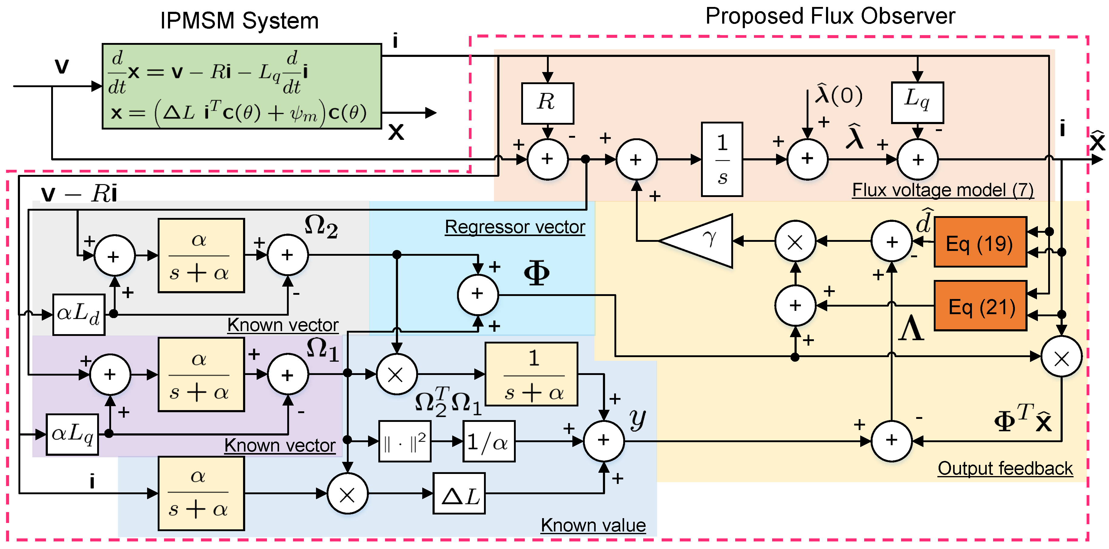
Its block diagram is depicted in Figure 1.
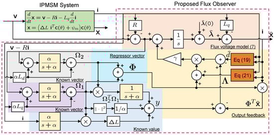
Figure 1.
Proposed nonlinear observer based on linear regression model.
As shown in the figure, the proposed observer consists of an open loop flux observer (7) and an output feedback loop. The output feedback loop plays a significant role to stable the observer, it consists the known filtered vector, value, and estimation variable .
Remark 1.
The state flux observer (23) has a driving term, , in which Φ contains the filtered variables, and . It has only two tuning parameters, γ and α.
Remark 2.
Remark 3.
Note that the cross-coupling effect was deliberately omitted for simplicity of the regression model. If the cross-coupling effect is considered in the model, it is very difficult to derive the regression model and it is complicated to apply to the real system. However, the performance of sensorless control is limited, due to the model error when the signal is injected in the low speed range.
4. Signal Injection Strategy
When the motor is low, it tends to be difficult to satisfy the PE condition. Then, the system is likely to become unstable. In short, poor performance at low speeds is directly related to the loss of the PE condition. Note, however, that the PE condition could be satisfied when high frequency signals are used. Typically, the d and q axis currents are constants during steady state. Nonetheless, oscillating high frequency signals are superimposed on the normal currents to meet the PE condition. Substituting (16) and (17) into (15), we have the following:
Using , , (3), and (5), we have the following:
Note from that regression vector plays a vital role in the PE condition [31]. The right side of (29) consists of three terms: two of them depend on the speed, , while the other one does not. Therefore, the two speed dependent terms are useless in the vicinity of zero speed. In the low speed region, we have the following:
To get a clear signal of , and must be alternating since the differential operator is applied to them. This means that the use of high frequency signal is inevitable.
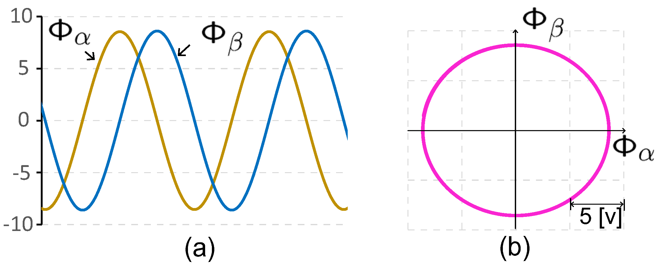
Consider the superimposed signals:
where and are the reference currents required for torque control, and and are high frequency signals. Note that and that the two injected signals differ in phase by . Then, (30) turns out to be the following:
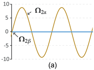
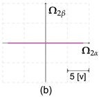
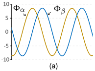
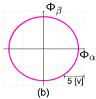
where . It is obvious that the trajectory of (33) forms a circle in the stationary frame as shown in Figure 2b. It corresponds to the level curve of a quadratic function with two equal eigenvalues. Consequently, the proposed regressor vector satisfies the PE condition, especially when the speed is zero. Compared to the previous observer [29], the previous regressor vector cannot satisfy the PE condition at zero speed by any signal injection methods. However, since the injection signal was considered, additional terms, such as and , are added to the proposed observer. It slightly increases the complexity of the observer and makes the stability analysis difficult.
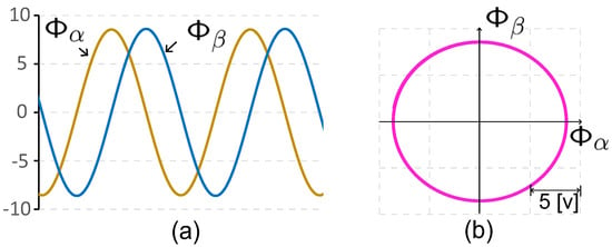
Figure 2.
The regressor vector with the injection signal at zero speed: (a) Time plots of and , and (b) its Lissajous pattern.
The comparison results of the proposed regression model with the previous model [29] are listed in Table 1. Excepting the vanishing disturbance term , all regression terms differentiate between two regression models. Note that the proposed regressor vector has current derivative terms in both directions (-axis). However, the previous regressor vector has one derivative term in the d-axis current. As a result, the Lissajous trajectories of two regressor vectors are different. The trajectory of the proposed regressor vector is drawn on a circle at standstill. It means the regressor vector satisfies the PE condition.

Table 1.
Comparison of the proposed regression model with the previous model.
5. Simulation and Experimental Results
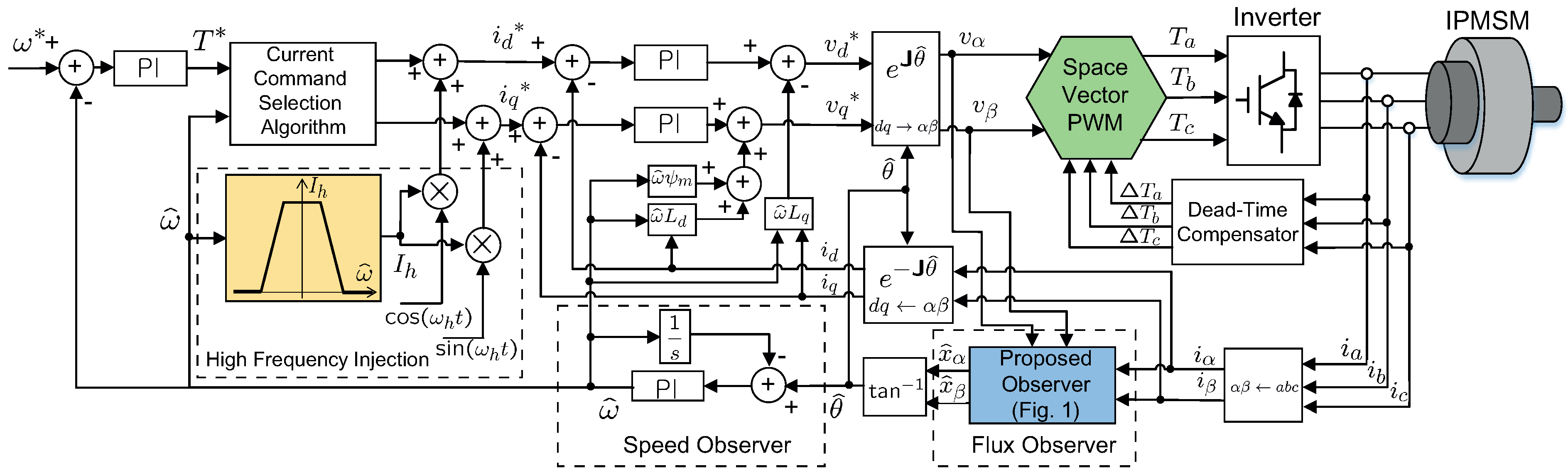
Figure 3 shows the sensorless control block diagram that includes the proposed flux observer. The current commands were calculated using the copper loss minimizing method [33]. Simulations and experiments were performed with the parameters of a real IPMSM listed in Table 2. High frequency sinusoidal currents are added to the -axis current reference only in the low speed region, 80 r/min. They are gradually decreased to zero as the speed increases. Thus, it realizes a seamless transition from the signal injection to the pure observer-based algorithm, and vice versa.

Figure 3.
Sensorless control block diagram for IPMSM that employs signal injection only in the low speed region.
Table 2.
Parameters of an interior PMSM and gains of the proposed observer used in the simulation and experiment.
The filter gain should be tuned above the frequency of the injection signal, . If the filter gain value is less than the injection frequency, the amplitude of the regressor vector is attenuated. It may diminish the signal-to-noise ratio. Additionally, the adaption gain should be selected in consideration of the whole operation range. The selection guideline was discussed in [29]. In the paper, the fixed adaption gain was used as 4.
5.1. Simulation Results
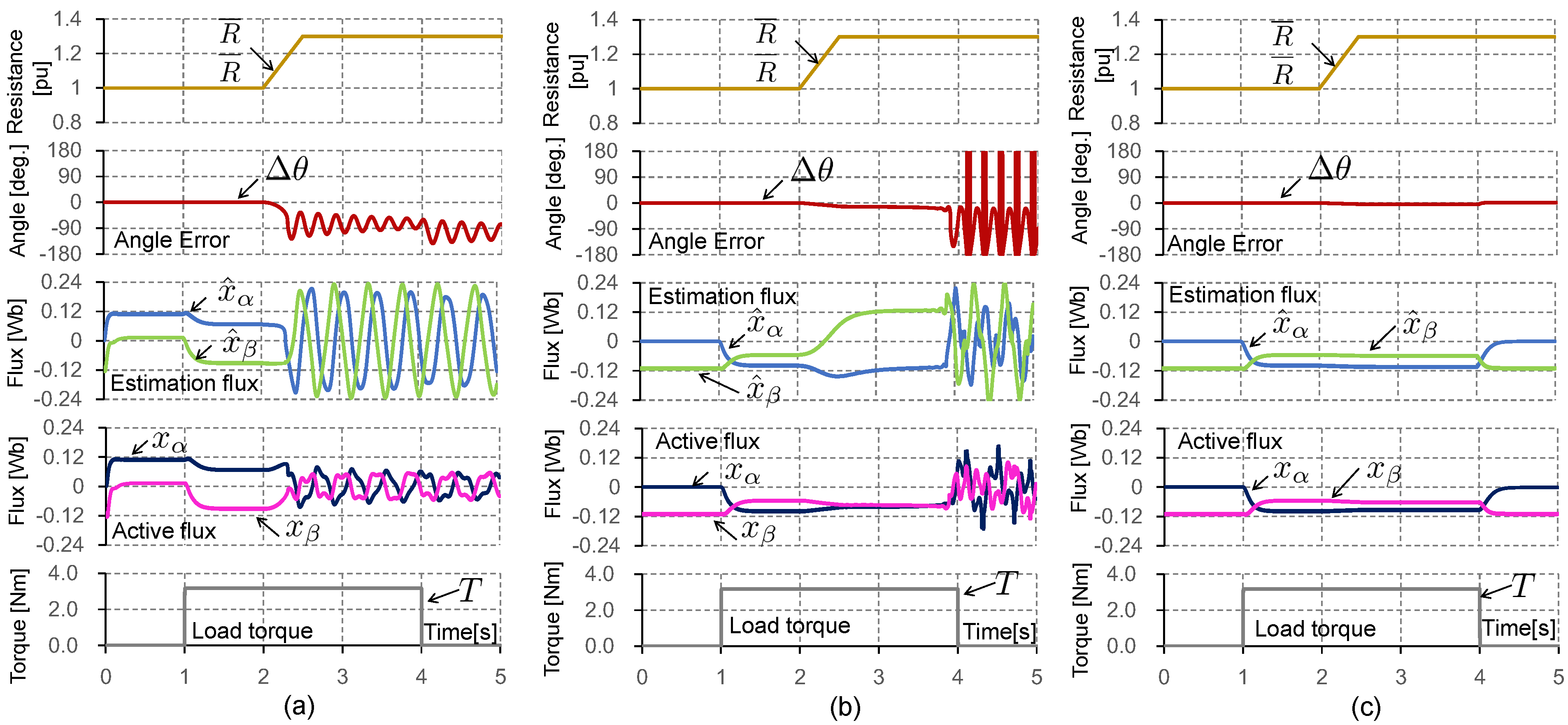
Simulations were performed using MATLAB Simulink. In Figure 4, zero speed control performances are compared with the Gopinath model flux observer [8], the previous observer based on regression model [29], and the proposed observer. In all cases, the high frequency signal was injected with the speed control mode, while 0.5 pu load torque was applied from 1 s to 4 s. To see the robustness, a 30% overly estimated resistor value was used in the observer after 2 s. As soon as the resistor value is not matched, unstable oscillations are observed with Gopinath model-based flux observer in Figure 4a. In the case of the previous regression-based observer, the estimated flux error gradually increases, due to the resistor value mismatch, and the observer becomes unstable after 2 s as shown in Figure 4b. On the other hand, stable results are obtained with the proposed scheme under all situations in Figure 4c. The resistance error causes 4 angle error.
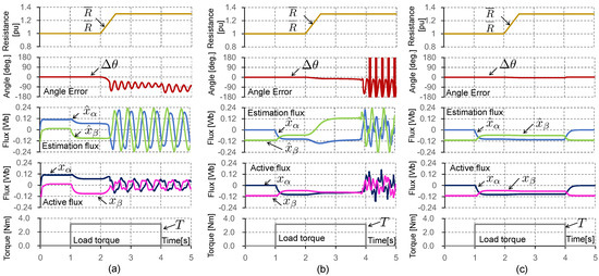
Figure 4.
Simulation results at zero speed under 0.5 pu load when the resistance is 30% erroneous: (a) Gopinath model flux observer [8], (b) previous observer based on regression model [29], and (c) proposed observer.
5.2. Experimental Results
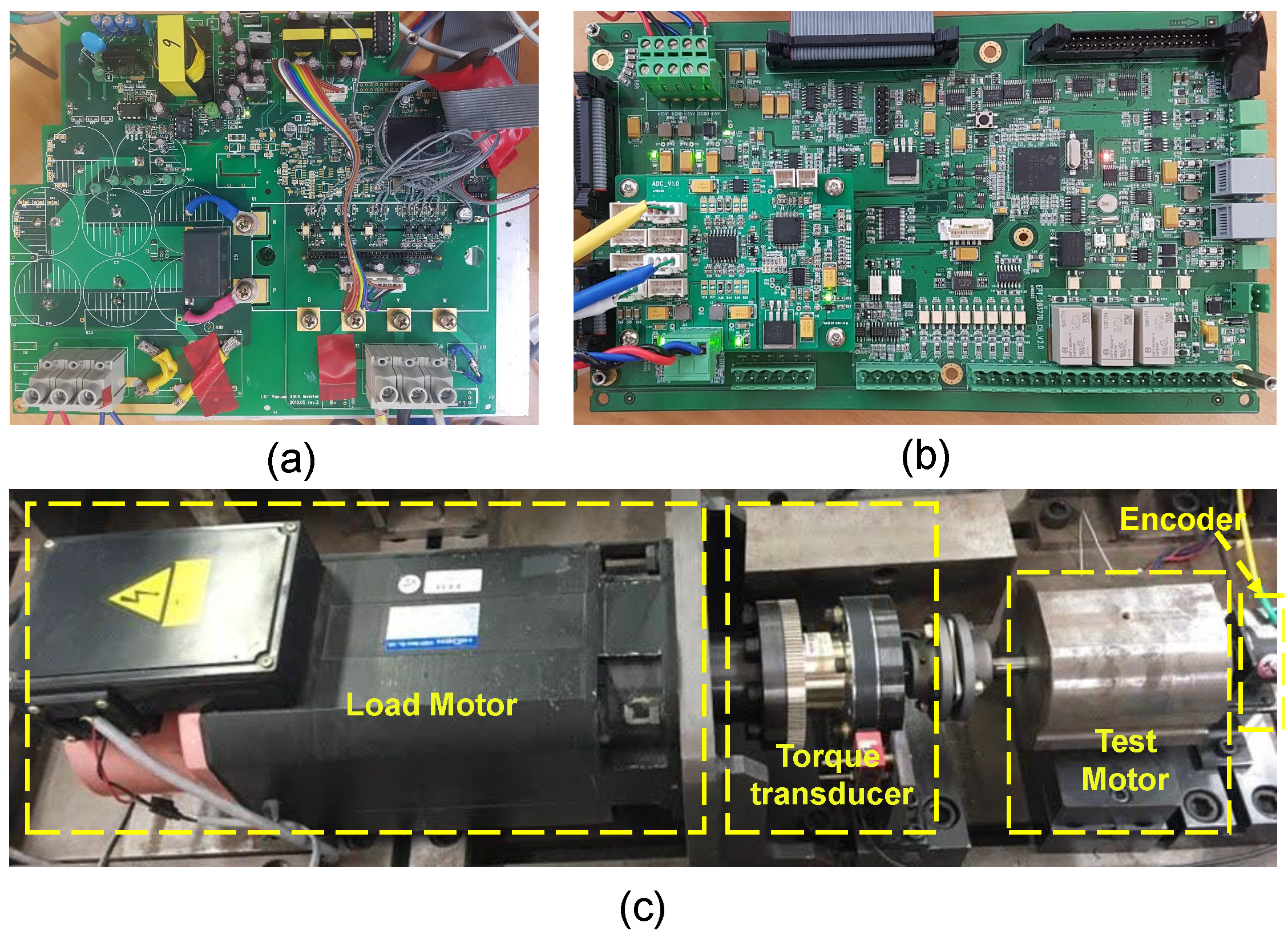
Figure 5 shows the inverter, dynamo set, and control board made with TMS320F28377. The pulse-width modulation (PWM) frequency was set 5 kHz, while the current sampling rate was 10 kHz. The analog to digital converter (ADC) was set in the 16 bit mode. The rotor angle and speed were measured by an encoder with 4000 pulse per revolution. The dead time was 2.0 s. The phase voltage was computed from the measured dc-link voltage and the PWM duty. In order to mitigate the inverter nonlinearity, the dead time and IGBT on-drop were carefully compensated [30,34].
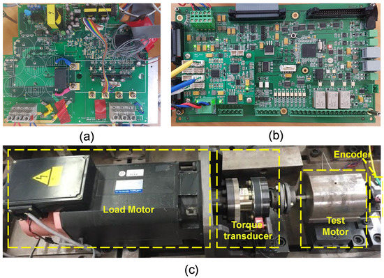
Figure 5.
Experimental environments: (a) inverter (b) control board, and (c) test bench.
Typically, the d-q axis inductance of PMSM varies significantly along with core saturation, due to the stator current. The variation causes a difference between the real value and the inductance parameter used in the observer. It makes the estimated angle offset error. To mitigate the effect of the inductance variation on the observer, the d-q axis inductance parameters were continuously updated through the lookup table.
To investigate the behavior of and , three different sets of current references were injected when the motor was at standstill under no load condition: , , and . Figure 6a shows the current plots versus time, while (b), (c) and (d) show Lissajous plots of and . In the first case, only the d-axis current was utilized. In the second case, both d and q axis currents were utilized. However, they were in the same phase. The last one is a case when the d and q axis currents reference differ in phase by 90, (31)–(33). In the last case, a trajectory of and was drawn, similar to a circle. It can be represented by (33). The regressor vector satisfied the PE condition [26], It yielded a most suitable contour for the PE condition.
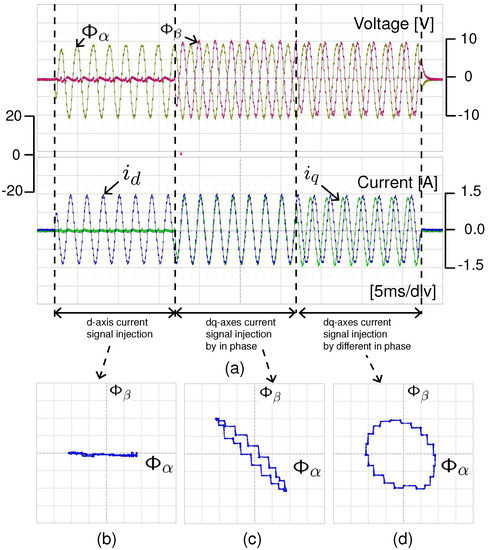
Figure 6.
Plots of currents and regression functions: (a) currents and (b–d) Lissajous contours of and .
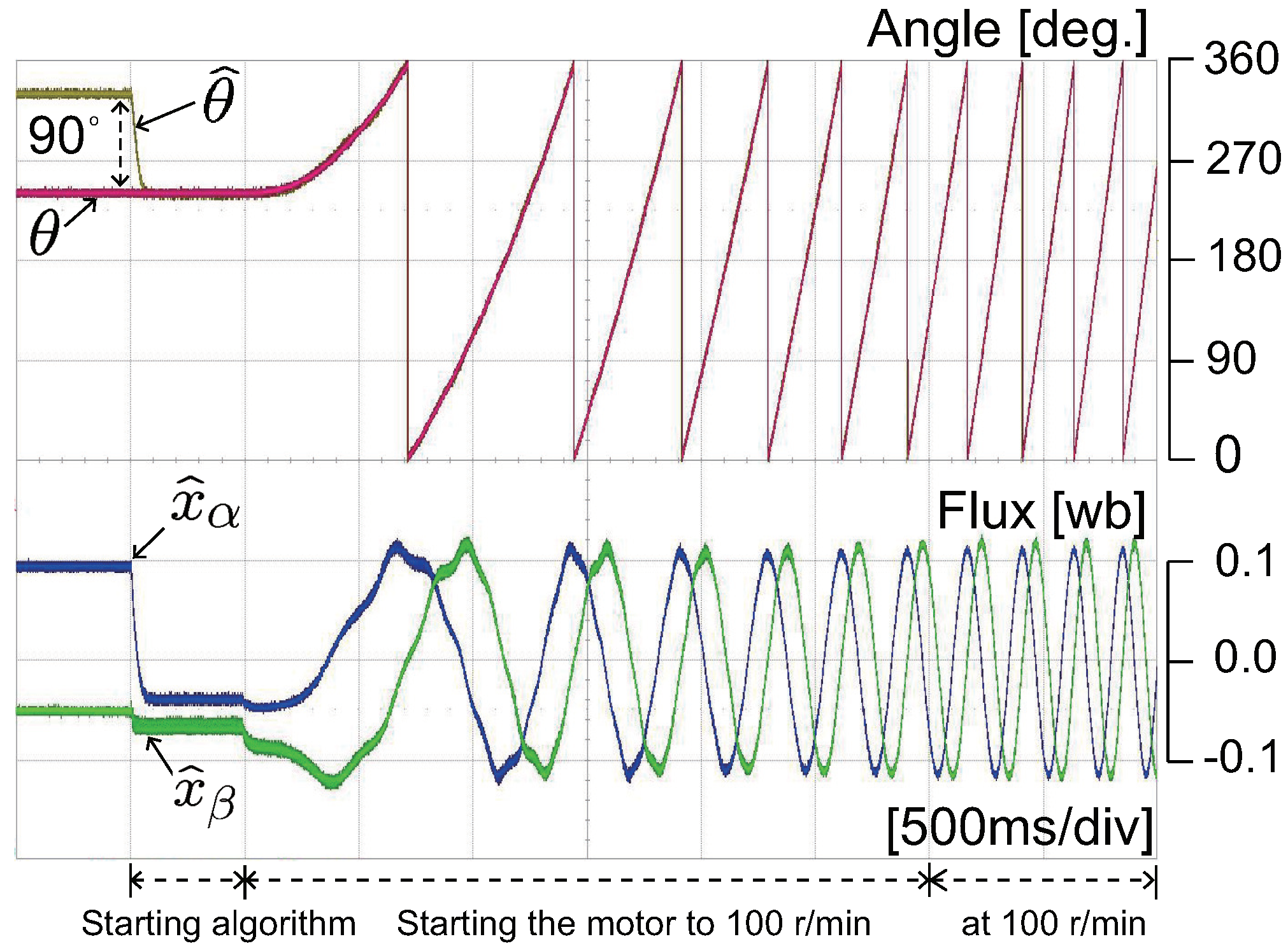
Figure 7 shows a case of starting in the speed control mode under no load condition. Initially, the angle estimation error was 90. A starting algorithm was executed during the first 500 ms. In that period, no control action was taken, but the angle was estimated with high frequency current injection. The plot shows us that the angle error converged at the zero speed state. Then, the speed was increased to 100 r/min. It should be noted that the convergence is guaranteed only when the angle error is less than at standstill. When the angle error is larger than at standstill, another polarity checking algorithm is required [35].
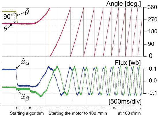
Figure 7.
Angle and active flux estimation at the starting under no load condition when the initial angle error is .
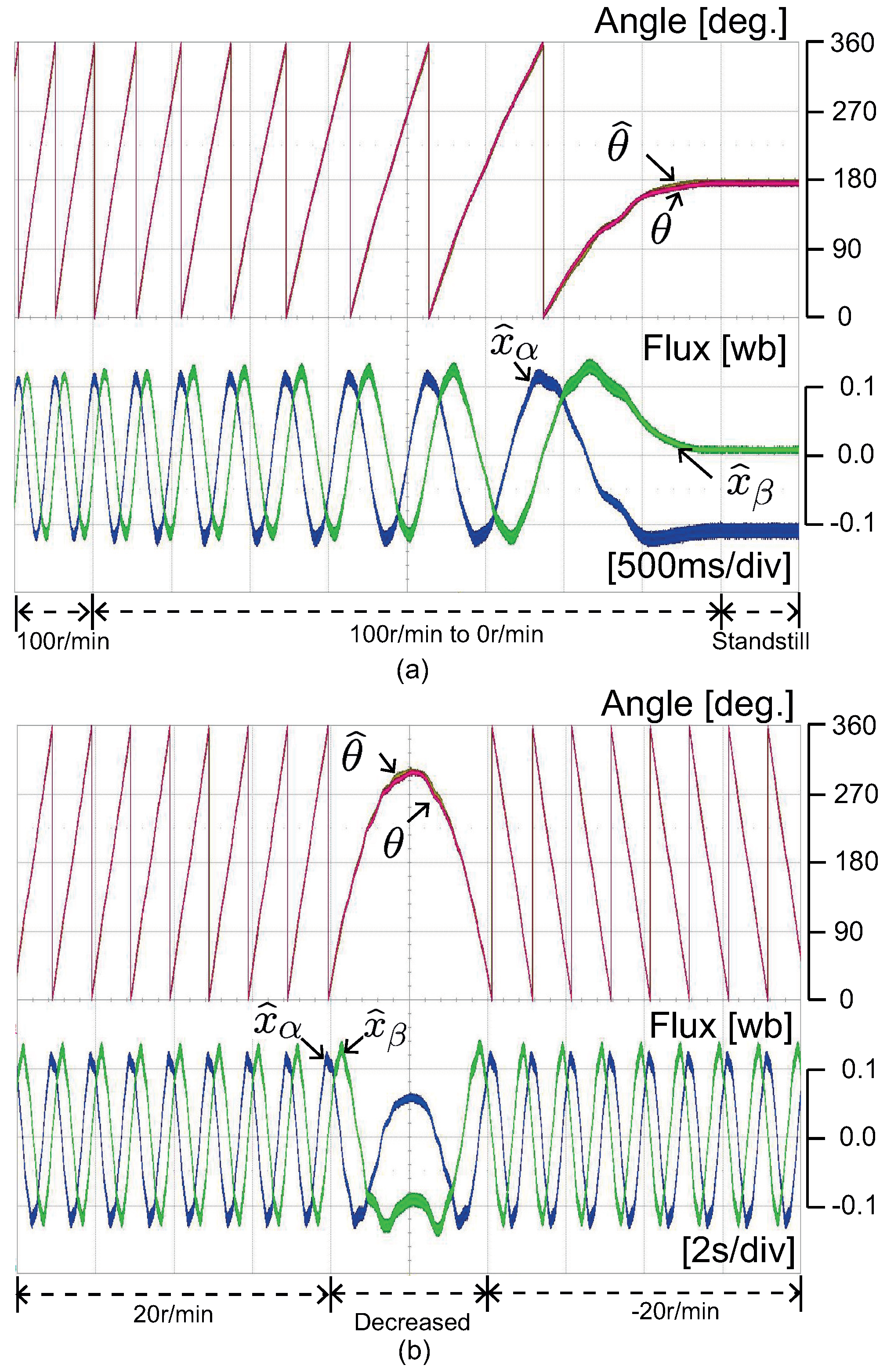
Figure 8a shows a zero speed control performance from 20 r/min to standstill. Figure 8b shows a speed control performance from 20 r/min to −20 r/min without a load. The angle was estimated correctly, even at zero speed.
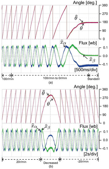
Figure 8.
Speed under no load condition control performance under no-load condition: (a) Standstill speed control, and (b) reverse speed control from 20 r/min to −20 r/min.
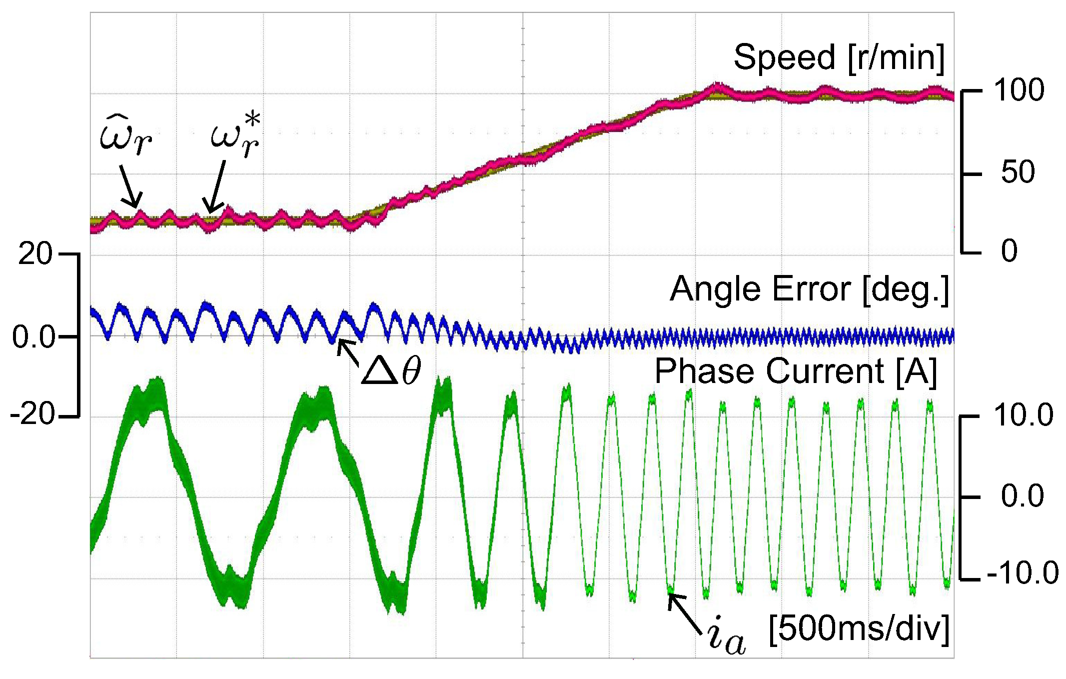
Figure 9 shows a speed transition from 20 r/min to 100 r/min under 1.0 pu load torque. Note that high frequency signal was injected up to 80 r/min. The presence of high frequency signal can be checked by the thickness of phase current. Since the amplitude of injected signal decreased steadily from 40 r/min to 80 r/min, its presence was clearly seen at 20 r/min. Figure 10 shows a zero speed control performance when 0.9 pu load torque was applied and removed during 2.4 7.5 s. Speed hunting was not observed, except at the moment of the load torque transition. Note that the magnitude of a-phase current increased in response to the step load, and that the angle error did not exceed 25 under the load.
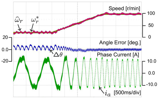
Figure 9.
Speed transition from 20 r/min to 100 r/min under 1.0 pu load torque.

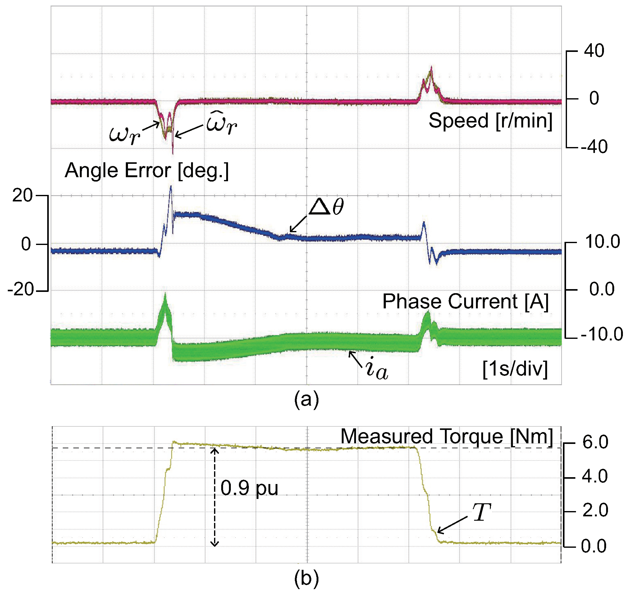
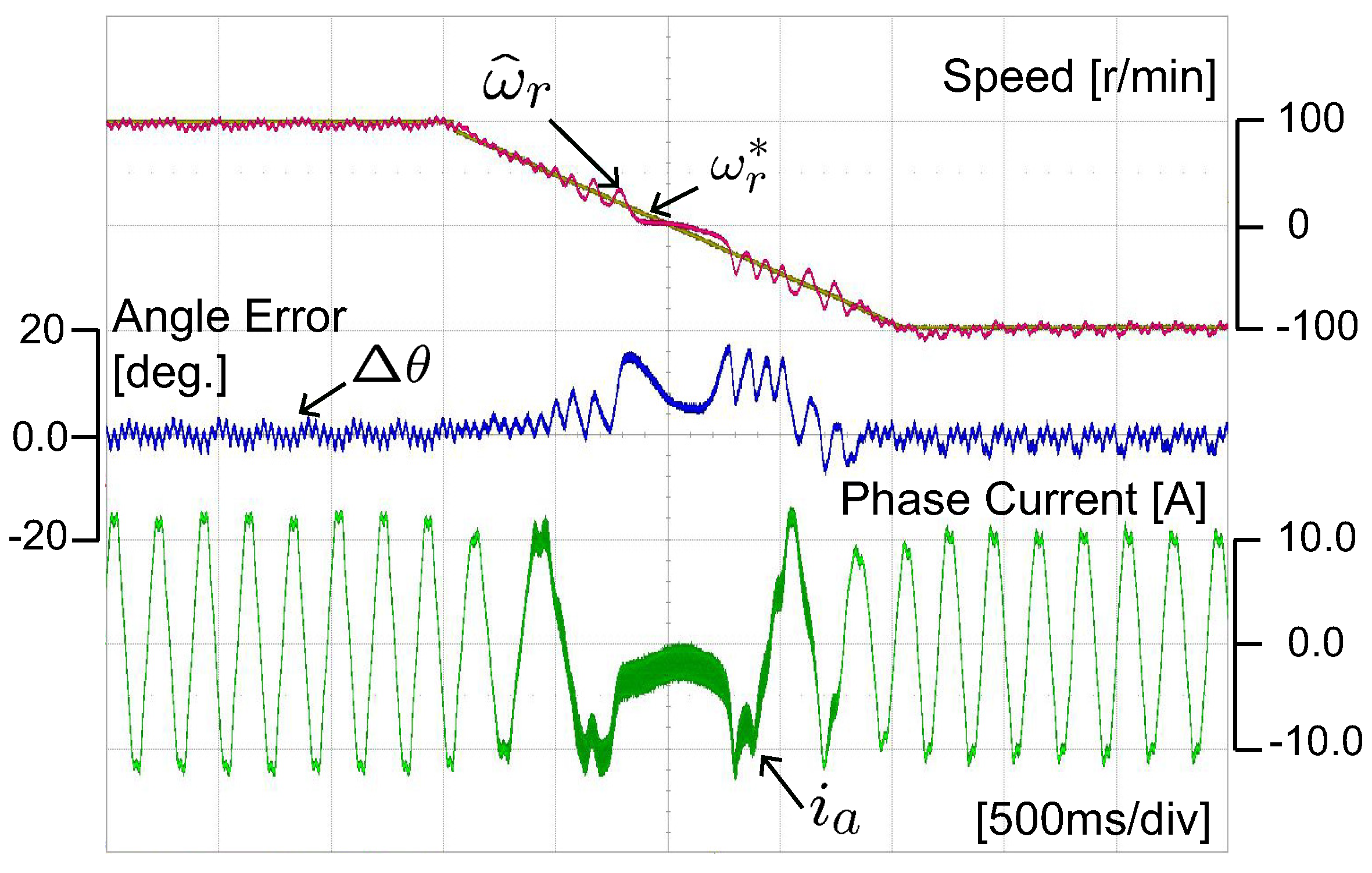
Figure 10.
Zero speed under no load condition. Control performance under 0.9 pu load: (a) speed, angle error, a-phase current, and (b) load torque.
Figure 11 shows the speed and current responses when the speed changed from 100 to −100 r/min under 1.0 pu load condition. At the zero speed, current hunting was not observed, and the angle error was regulated under . It can be seen from a-phase current that high frequency signal was injected only in the low frequency region, r/min. As shown in Figure 3, the amplitude of injected signal changed gradually over r/min and –80 –40 r/min. It demonstrates a seamless transition from a pure model-based sensorless control to a signal injection method, and vice versa.
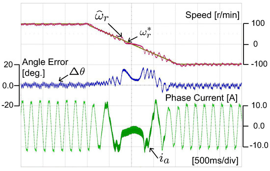
Figure 11.
Speed transition under no load condition from 100 to −100 r/min under 1.0 pu load.
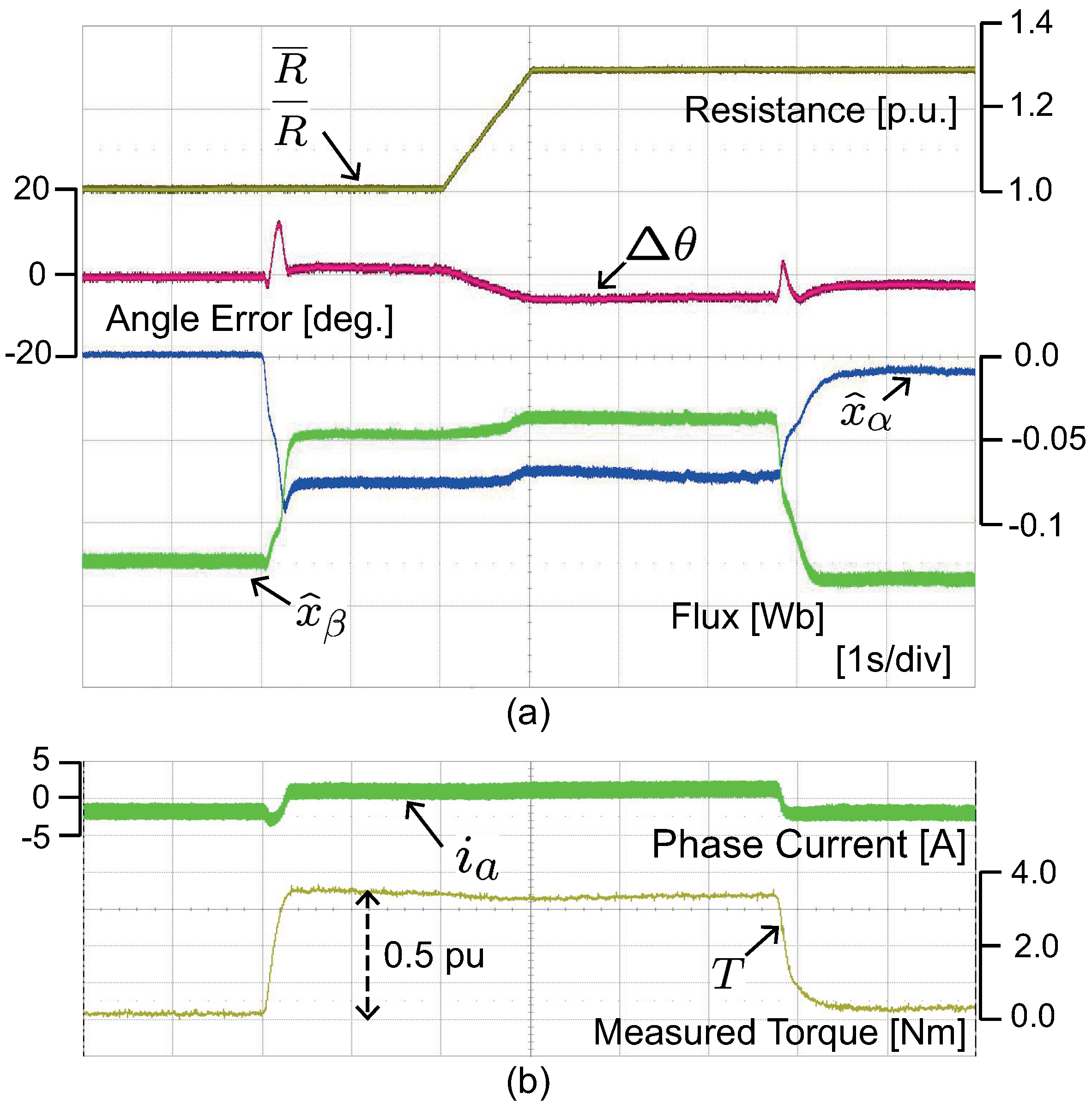
Figure 12 shows a zero speed control performance under 0.5 pu load when the estimate of the coil resistance changed 30%, erroneously. The angle error, increased slightly with the error in R. This experimental result matches well with the simulation result shown in Figure 4c. It is a meaningful experimental result. In the model-based sensorless method, an erroneous parameter in resistance has a significant impact on the estimation angle error and stability at the low-speed region, which is included at zero speed. To mitigate the effect of the mismatch resistance on the estimation angle and stability in the low speed region, the stator resistance was estimated [36]. However, it makes for a complicated system and requires time-varying adaption gain depending on the operation region. In contrast, the proposed method with the injection signal has low sensitivity to erroneous resistance values.
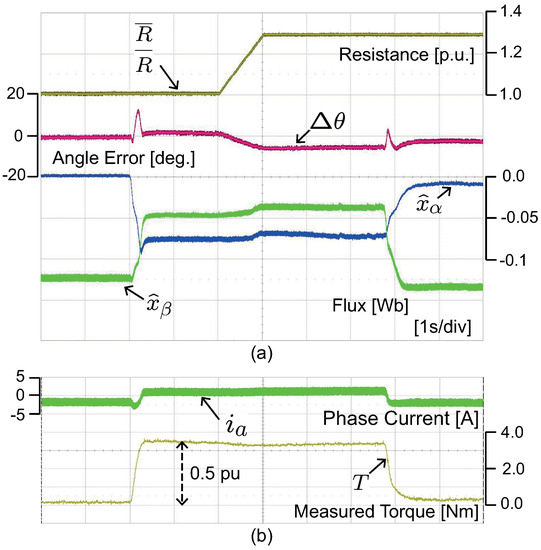
Figure 12.
Zero speed control performance under 0.5 pu load when the resistor estimation error increased to 30%: (a) The erroneous resistance, estimated angle error, and estimated flux and (b) phase current and measured torque.
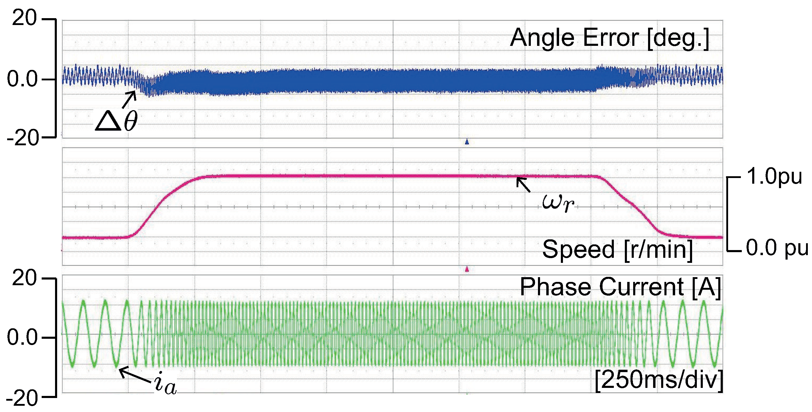
Figure 13 shows the sensorless performance when rapidly changing the motor speed. The estimated angle was adjusted within the tolerable range when the motor was changed from 400 r/min (0.2 pu) to 2000 r/min (1.0 pu) for 250 ms with rated load.
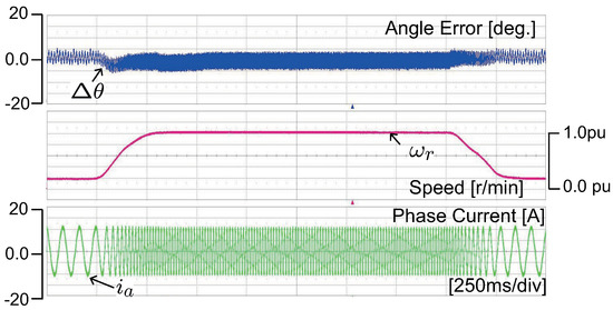
Figure 13.
Speed transition from 400 r/min to 2000 r/min (1.0 pu) under the rated load.
6. Conclusions
The saliency of IPMSM dynamics is dealt with elaborately by the active flux, and a vector, . A linear regression form is derived from the square of the active flux, . The high pass filter acts a role of suppressing a constant rotor flux term, . The term with rotor saliency, is carefully treated in the process of applying the gradient rule. The perturbation term, which is caused by the derivative of the d-axis current, is also taken into account when constructing an observer.
The proposed regressor vector includes and . It allows high frequency signal injection in the d-axis, as well as the q-axis. The dual excitation enhances the chance of satisfying the PE condition. Therefore, the high-frequency signal can be injected when it is necessary and turned off as the speed increases. Therefore, it provides seamless transitions between the signal injection to observer based modes. It enhances the low speed performance under loaded condition. It was validated through simulation and experiments with 30% resistance error. The motor was controlled successfully at standstill.
Funding
This work was supported by the National Research Foundation of Korea (NRF) grant funded by the Korean government (MSIT) (NRF-2021R1I1A3059676).
Conflicts of Interest
The author declares no conflict of interest.
Abbreviations
The following abbreviations are used in this manuscript:
| Stationary axis reference frame quantities | |
| Synchronous axis reference frame quantities | |
| R | Resistance of stator winding |
| d-axis and q-axis inductance of stator winding | |
| d and q-axes stator flux linkage in the synchronous frame | |
| Stator winding resistance | |
| d and q-axes self-inductance | |
| Stator flux in the stationary frame | |
| Initial Stator flux | |
| Active flux in the stationary frame | |
| Rotor flux angle | |
| Estimation rotor flux angle error | |
| Electrical speed and mechanical speed | |
| Injection current magnitude | |
| Injection current frequency | |
| T | Shaft torque |
| Adaptation gain of observer | |
| Filter gain | |
| Differential operator | |
| PMSMs | Permanent-magnet synchronous motors |
| IPMSM | Interior permanent-magnet synchronous motor |
| SPMSM | Surface-mount PMSM |
| EMF | Electromotive force |
| PE | Persistence of excitation |
| FEM | Finite-element method |
| LPF | Low pass filter |
| BPF | Band-pass filter |
Appendix A. Linear Regression Derivation Process
Applying Lemma in Appendix B to the first term on the right-hand side of (12), we have the following:
Similarly, the left-hand side of (12) is equal to the following:
Appendix B. Swapping Lemma
Lemma A1.
Assume that are differentiable and that is a constant. Then, we have the following:
References
- Chen, S.; Zhang, X.; Wu, X.; Tan, G.; Chen, X. Sensorless Control for IPMSM Based on Adaptive Super-Twisting Sliding-Mode Observer and Improved Phase-Locked Loop. Energies 2019, 12, 1225. [Google Scholar] [CrossRef] [Green Version]
- Liu, J.; Nondahl, T.; Schmidt, P.; Royak, S.; Harbaugh, M. Rotor Position Estimation for Synchronous Machines Based on Equivalent EMF. IEEE Trans. Ind. Appl. 2011, 47, 1310–1318. [Google Scholar]
- Bao, D.; Wu, H.; Wang, R.; Zhao, F.; Pan, X. Full-Order Sliding Mode Observer Based on Synchronous Frequency Tracking Filter for High-Speed Interior PMSM Sensorless Drives. Energies 2020, 13, 6511. [Google Scholar] [CrossRef]
- Usama, M.; Kim, J. Improved Self-Sensing Speed Control of IPMSM Drive Based on Cascaded Nonlinear Control. Energies 2021, 14, 2205. [Google Scholar] [CrossRef]
- Xu, Z.; Zhang, T.; Bao, Y.; Zhang, H.; Gerada, C. A Nonlinear Extended State Observer for Rotor Position and Speed Estimation for Sensorless IPMSM Drives. IEEE Tran. Power Electron. 2020, 35, 733–743. [Google Scholar] [CrossRef]
- Kim, J.; Jeong, I.; Nam, K.; Yang, J.; Hwang, T. Sensorless Control of PMSM in a High-Speed Region Considering Iron Loss. IEEE Trans. Ind. Electron. 2015, 62, 6151–6159. [Google Scholar] [CrossRef]
- Hasegawa, M.; Hatta, H.; Matsui, K. Adaptive flux observer on stator frame and its design based on /spl gamma/-positive real problem for sensorless IPMSM drives. In Proceedings of the 31st Annual Conference of IEEE Industrial Electronics Society, IECON 2005, Raleigh, NC, USA, 6–10 November 2005. [Google Scholar]
- Boldea, I.; Paicu, M.C.; Andreescu, G.D. Active Flux Concept for Motion-Sensorless Unified AC Drives. IEEE Trans. Power Electron. 2008, 23, 2612–2618. [Google Scholar] [CrossRef]
- Wang, S.; Zhao, J.; Yang, K. High Frequency Square-Wave Voltage Injection Scheme-Based Position Sensorless Control of IPMSM in the Low- and Zero- Speed Range. Energies 2019, 12, 4776. [Google Scholar] [CrossRef] [Green Version]
- Guo, L.; Yang, Z.; Lin, F. A Novel Strategy for Sensorless Control of IPMSM with Error Compensation Based on Rotating High Frequency Carrier Signal Injection. Energies 2020, 13, 1919. [Google Scholar] [CrossRef]
- Choi, J.; Nam, K. Wound Synchronous Machine Sensorless Control Based on Signal Injection into the Rotor Winding. Energies 2018, 11, 3278. [Google Scholar] [CrossRef] [Green Version]
- Chen, J.; Yang, S.; Tu, J. Comparative Evaluation of a Permanent Magnet Machine Saliency-Based Drive with Sine-Wave and Square-Wave Voltage Injection. Energies 2018, 11, 2189. [Google Scholar] [CrossRef] [Green Version]
- Mubarok, M.S.; Liu, T.-H.; Tsai, C.-Y.; Wei, Z.-Y. A Wide-Adjustable Sensorless IPMSM Speed Drive Based on Current Deviation Detection under Space-Vector Modulation. Energies 2020, 13, 4431. [Google Scholar] [CrossRef]
- Foo, G.; Rahman, M.F. Sensorless Sliding-Mode MTPA Control of an IPM Synchronous Motor Drive Using a Sliding-Mode Observer and HF Signal Injection. IEEE Tran. Ind. Electron. 2010, 57, 1270–1278. [Google Scholar] [CrossRef]
- Andreescu, G.D.; Pitic, C.I.; Blaabjerg, F.; Boldea, I. Combined Flux Observer With Signal Injection Enhancement for Wide Speed Range Sensorless Direct Torque Control of IPMSM Drives. IEEE Trans. Energy Convers. 2008, 23, 393–402. [Google Scholar] [CrossRef]
- Barnard, F.J.W.; Villet, W.T.; Kamper, M.J. Hybrid Active-Flux and Arbitrary Injection Position Sensorless Control of Reluctance Synchronous Machines. IEEE Trans. Ind. Appl. 2015, 51, 3899–3906. [Google Scholar] [CrossRef]
- Silva, C.; Asher, G.M.; Sumner, M. Hybrid rotor position observer for wide speed-range sensorless PM motor drives including zero speed. IEEE Trans. Ind. Electron. 2006, 53, 373–378. [Google Scholar] [CrossRef]
- Yousefi-Talouki, A.; Pescetto, P.; Pellegrino, G.; Boldea, I. Combined Active Flux and High-Frequency Injection Methods for Sensorless Direct-Flux Vector Control of Synchronous Reluctance Machines. IEEE Trans. Power Electron. 2018, 33, 2447–2457. [Google Scholar] [CrossRef]
- Tuovinen, T.; Hinkkanen, M. Adaptive Full-Order Observer With High-Frequency Signal Injection for Synchronous Reluctance Motor Drives. IEEE J. Emerg. Sel. Top. Power Electron. 2014, 2, 181–189. [Google Scholar] [CrossRef] [Green Version]
- Sun, Y.; Preindl, M.; Sirouspour, S.; Emadi, A. Unified wide-speed sensorless scheme using nonlinear optimization for IPMSM drives. IEEE Trans. Power Electron. 2017, 32, 6308–6322. [Google Scholar] [CrossRef]
- Peng, F.; Yao, Y.; Wang, Z.; Huang, Y.; Yang, H.; Xie, B. Position Estimation Method of IPMSM in Full Speed Range by Simplified Quadratic Optimization. IEEE Access 2020, 8, 109964–109975. [Google Scholar] [CrossRef]
- Chen, J.; Chen, S.; Wu, X.; Tan, G.; Hao, J. A Super-Twisting Sliding-Mode Stator Flux Observer for Sensorless Direct Torque and Flux Control of IPMSM. Energies 2019, 12, 2564. [Google Scholar] [CrossRef] [Green Version]
- Ortega, R.; Praly, L.; Astolfi, A.; Lee, J.; Nam, K. Estimation of rotor position and speed of permanent magnet synchronous motors with guaranteed stability. IEEE Trans. Control Syst. Technol. 2011, 19, 601–614. [Google Scholar] [CrossRef]
- Dib, W.; Ortega, R.; Malaize, A.J. Sensorless control of permanent-magnet synchronous motor in automotive applications: Estimation of the angular position. In Proceedings of the IECON 2011—37th Annual Conference on IEEE Industrial Electronics Society, Melbourne, VIC, Australia, 7–10 November 2011; pp. 728–733. [Google Scholar]
- Lee, J.; Hong, J.; Nam, K.; Ortega, R.; Praly, L.; Astolfi, A. Sensorless Control of Surface-Mount Permanent-Magnet Synchronous Motors Based on a Nonlinear Observer. IEEE Trans. Power Electron. 2010, 25, 290–297. [Google Scholar]
- Bobtsov, A.; Pyrkin, A.; Ortega, R.; Vukosavic, S.; Stankovic, A.M.; Panteley, E.V. A Robust Globally Convergent Postion Observer for the Permanent Magnet Synchronous Motor. Automatica 2015, 61, 47–54. [Google Scholar] [CrossRef]
- Bobtsov, A.; Pyrkin, A.; Ortega, R. A new approach for estimation of electrical parameters and flux observation of permanent magnet synchronous motors. Int. J. Adapt. Control Signal Process 2015, 30, 1434–1448. [Google Scholar] [CrossRef]
- Choi, J.; Nam, K.; Bobtsov, A.A.; Pyrkin, A.; Ortega, R. Robust Adaptive Sensorless Control for Permanent-Magnet Synchronous Motors. IEEE Trans. Power Electron. 2017, 30, 3989–3997. [Google Scholar] [CrossRef]
- Choi, J.; Nam, K.; Bobtsov, A.A.; Ortega, R. Sensorless Control of IPMSM Based on Regression Model. IEEE Trans. Power Electron. 2019, 34, 9191–9201. [Google Scholar] [CrossRef]
- Nam, K.H. AC Motor Control and Electric Vehicle Application; CRC Press: Boca Raton, FL, USA, 2018; ISBN 9781138712492. [Google Scholar]
- Ortega, R.; Praly, L.; Aranovskiy, S.; Yi, B.; Zhang, W. On dynamic regressor extension and mixing parameter estimators: Two Luenberger observers interpretations. Automatica 2018, 95, 548–551. [Google Scholar] [CrossRef]
- Sastry, S.; Bodson, M. Adaptive Control: Stability, Convergence and Robustness; Prentice-Hall: London, UK, 1989; ISBN 9780486482026. [Google Scholar]
- Jung, S.; Hong, J.; Nam, K. Current Minimizing Torque Control of the IPMSM Using Ferrari’s Method. IEEE Trans. Power Electron. 2013, 28, 5603–5617. [Google Scholar] [CrossRef]
- Seyyedzadeh, S.M.; Shoulaie, A. Accurate Modeling of the Nonlinear Characteristic of a Voltage Source Inverter for Better Performance in Near Zero Currents. IEEE Trans. Ind. Electron. 2019, 66, 71–78. [Google Scholar] [CrossRef]
- Li, Y.; Wu, H.; Xu, X.; Sun, X.; Zhao, J. Rotor Position Estimation Approaches for Sensorless Control of Permanent Magnet Traction Motor in Electric Vehicles: A Review. World Electr. Veh. J. 2021, 12, 9. [Google Scholar] [CrossRef]
- Rashed, M.; MacConnell, P.F.A.; Stronach, A.F.; Acarnley, P. Sensorless Indirect-Rotor-Field-Orientation Speed Control of a Permanent-Magnet Synchronous Motor With Stator-Resistance Estimation. IEEE Trans. Ind. Electron. 2007, 54, 1664–1675. [Google Scholar] [CrossRef]

Publisher’s Note: MDPI stays neutral with regard to jurisdictional claims in published maps and institutional affiliations. |
© 2021 by the author. Licensee MDPI, Basel, Switzerland. This article is an open access article distributed under the terms and conditions of the Creative Commons Attribution (CC BY) license (https://creativecommons.org/licenses/by/4.0/).