Article

Novel Deperming Protocols to Reduce Demagnetizing Time and Improve the Performance for the Magnetic Silence of Warships

1
Department of Electrical Engineering, Dong Eui University, Busan 47340, Korea
2
Department of Electrical Engineering, Pusan National University, Busan 47340, Korea
*
Author to whom correspondence should be addressed.
Energies 2021, 14(19), 6295; https://doi.org/10.3390/en14196295
Submission received: 19 August 2021 / Revised: 29 September 2021 / Accepted: 29 September 2021 / Published: 2 October 2021

Abstract

:
Magnetic silence of warships is necessary to prevent damage caused by the magnetic mines detecting the magnetic field of the warship. Anhysteretic and Deperm-ME protocols are used to reduce permanent magnetization among magnetic signals. However, they have some disadvantages. Therefore, this paper proposes an effective deperming protocol that is easily controlled and reduces the demagnetization time. A protocol composed of two Anhysteretic protocols is presented using the Preisach model to easily manage and ensure excellent performance. Each stage has its own advantages by considering the Preisach density distribution. In Stage 1, the existing magnetic history is erased, and the demagnetization time is reduced. In Stage 2, the demagnetization performance is improved. The effectiveness of the protocol was verified via simulations using the Preisach model and experiments using a specimen. When the proposed protocol was applied, the results were excellent when applying Anhysteretic and Deperm-ME. In addition, even if the number of magnetic fields was reduced by 4 and 8 in the proposed protocol, the demagnetization result was maintained. Therefore, if the proposed protocol is applied, excellent demagnetization results can be obtained and the time required to perform demagnetization can be reduced, thereby improving the operational capability of the warship.

1. Introduction

The magnetic signals of the warship consist of the induced magnetic field caused by the earth’s magnetic field during operation [1,2,3], eddy currents by rolling [4], and the permanent magnetization generated during the manufacturing process. Most of the signals are the induced and the permanent magnetic fields. The induced magnetization changes according to the position, course, and azimuth of the ship under the earth’s magnetic fields. The permanent magnetization was generated inside the warship, as shown in Figure 1a, owing to the external environment, such as the change of local magnetic properties by welding and cutting the hull of the ship during manufacturing. Since the magnetic mines installed in the sea detect these signals and attack the warship, the ship’s magnetization has to be reduced to a certain magnitude. In particular, the permanent magnetization is less than 50% of the induced magnetization.
In general, demagnetization is performed for magnetic treatment of the warship, and then the induced magnetization is removed through the degaussing. A coil was wound around the warship to reduce permanent magnetization, as shown in Figure 1b, and the demagnetization was performed by applying continuously alternating and decreasing magnetic fields. These magnetic fields are called the deperming protocol. As the magnetic sensor installed outside the ship can measure the induced magnetic field, it can be eliminated by applying a canceling current to the coil installed inside the ship [2,3]. After the permanent magnetization is sufficiently reduced by demagnetization, the induced magnetization is more easily compensated by the degaussing coils with less power required.
The ship’s magnetization consists of a Cartesian component, with mostly longitudinal and vertical components. In the case of demagnetization, it is generally used to reduce the longitudinal component. From the practical point of view, the result of demagnetization should reach less than half of the induced magnetic field component. The vertical component is usually compensated by degaussing coils but since a submarine does not have degaussing coils, it is magnetized in the opposite direction of the earth’s magnetic field to eliminate the effect.
The most commonly used protocols for demagnetization are Anhysteretic Deperm, Deperm-ME, and Flash-D [5,6,7]. Flash-D is mainly used in submarines without degaussing coils, while others are used in warships equipped with degaussing coils. Several recent studies have shown that Deperm-ME performs better than Anhysteretic Deperm [8]. However, since complex control is required by the exponential function, it is not easy to use in the Navy. Therefore, a deperming protocol with better performance and easy control is needed. In addition, if the demagnetization time can be reduced, the operational capabilities of the warships can be improved.
This paper proposes an effective deperming protocol that is easy to control and can reduce the demagnetization time by using the Preisach model. The Preisach model can represent the hysteresis characteristics by considering the interactions between the magnetic particles inside the material. Therefore, it is suitable for demagnetization research. Moreover, in this paper, the influence of the earth’s magnetic field is removed. There are two reasons. The first is that the effect is compensated by degaussing systems after demagnetization. Second, the magnitude of the earth’s magnetic fields varies depending on the operation regions. Therefore, only an effective deperming protocol was studied in this paper.
The proposed protocol consists of two Anhysteretic protocols. The first protocol starts with a high magnetic field level to erase the previous history. Additionally, it operates in areas of low Preisach density, reducing the demagnetization time by decreasing unnecessary magnetic fields. The second protocol improves the demagnetization performance by drawing small traces in an area with high Preisach density distributions.
Simulations were performed using a program that combines the Preisach model and the Finite Element Method (FEM) to compare the proposed protocol with Anhysteretic and Deperm-ME. After applying each protocol, the distributions of the permanent magnetization were analyzed. In addition, experiments were performed in a scaled-down Magnetic Treatment Facility (MTF) test room in which the earth’s magnetic field and external influences were removed to verify the simulation results.

2. Proposed Deperming Protocol Using the Preisach Model
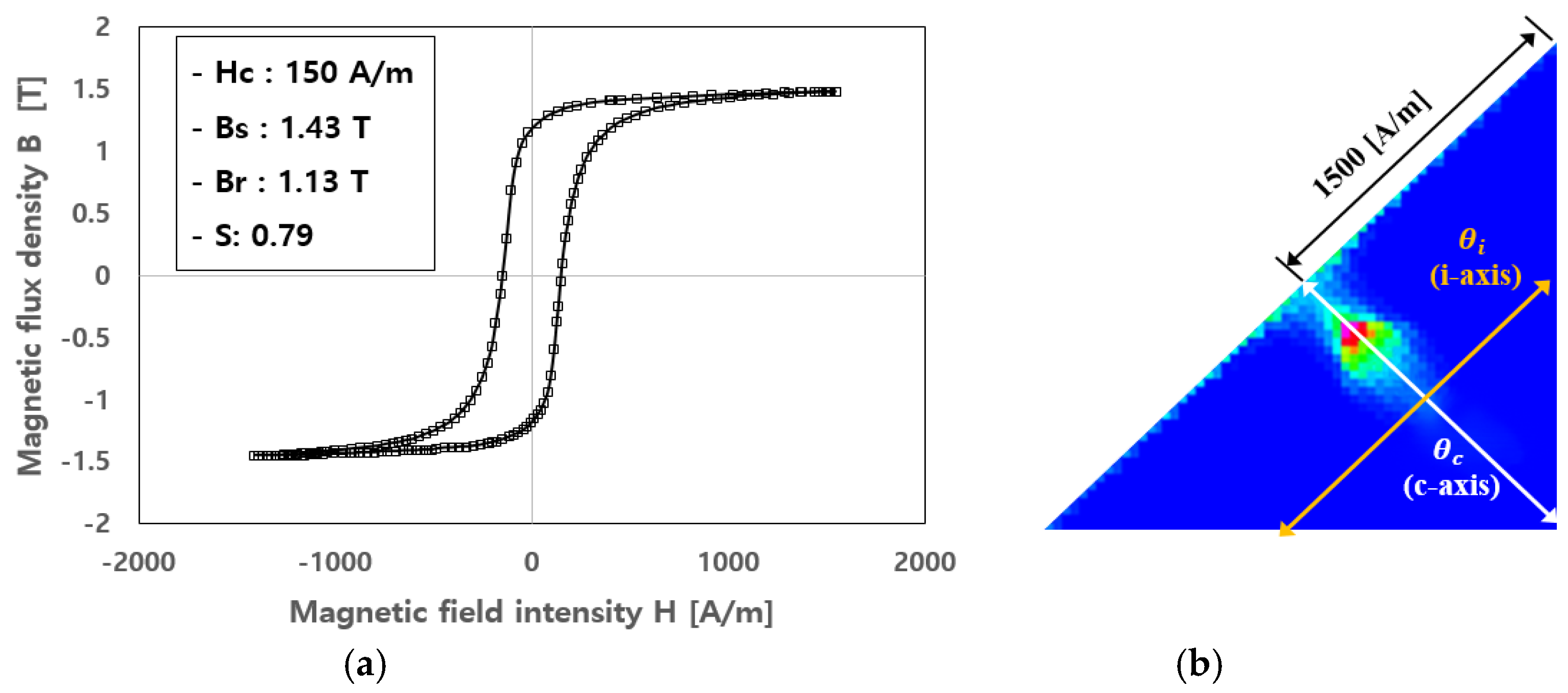
2.1. Preisach Model

The Preisach model was adopted in this research because it considers the coercive force and interactions between magnetic domains. The demagnetization process is also analyzed through the Jiles–Atherton model, which is one of the hysteresis modeling methods [9]. However, since it is difficult to consider the density distribution of magnetic materials, the Jiles–Atherton model is intuitively used for simulation rather than development of deperming protocols. On the other hand, the Preisach model calculates the amount of magnetization by integrating the density of hysterons corresponding to magnetic particles. As shown in Figure 2, the magnetic properties were represented by the density distribution of hysterons considering coercive force and interaction forces. Each hysteron is an element that can take only two values ((−1,1), (0,1)—depending on the model design decision) [10].
For example, there were hysterons with small coercive force and no interaction at P1. However, if there are interactions between hysterons, some hysterons will be shifted, such as those at P2. That is, along an interaction field axis, hysterons having the same coercive force had different interaction forces. Similarly, hysterons located on the same coercivity field axis had the same interaction force. Hysterons with larger coercive force were located at positions P3 and P4.

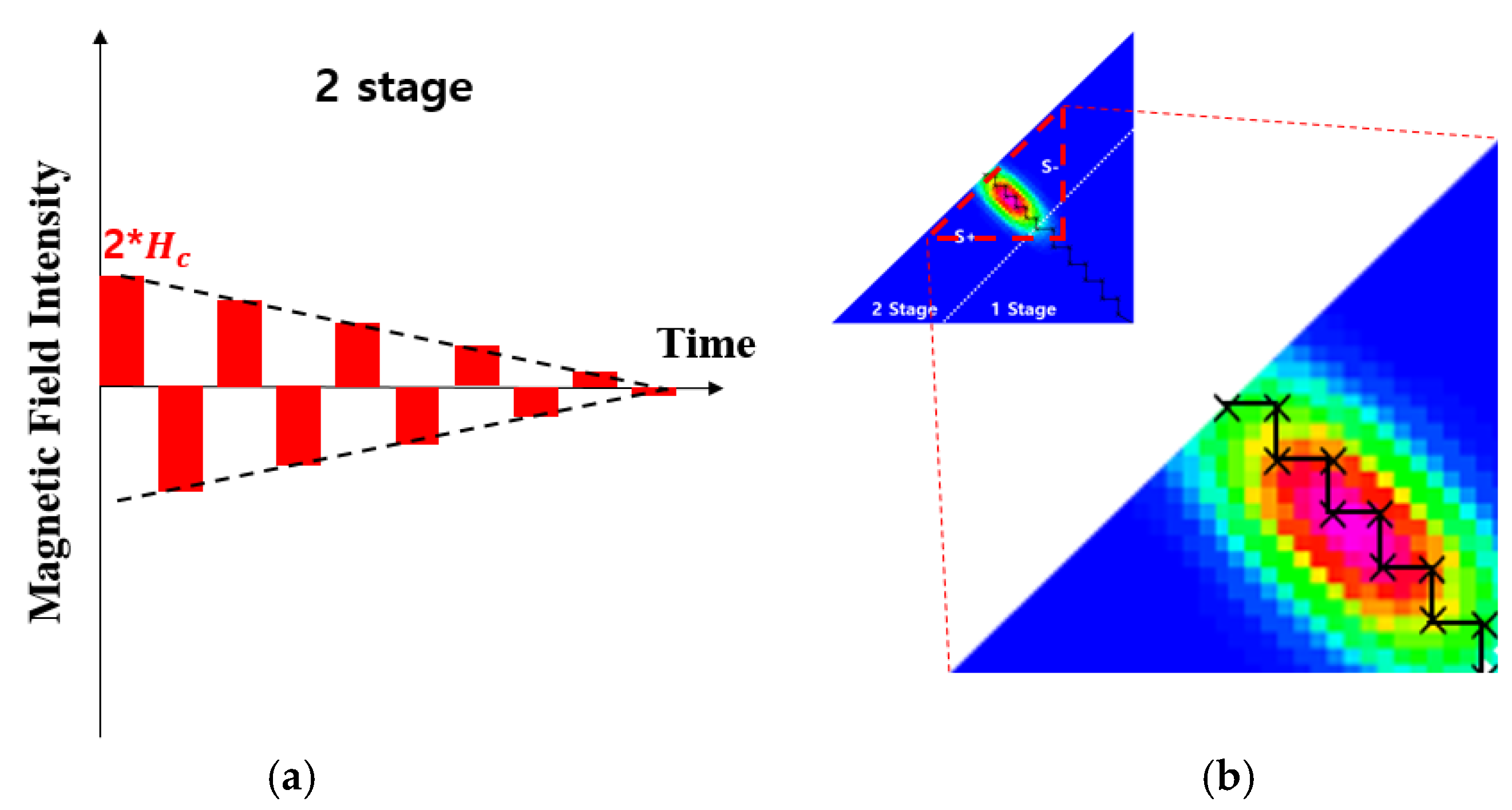
2.2. Conventional Deperming Protocols

Figure 3 shows the conventional deperming protocols: Anhysteretic Deperm and Deperm-ME. Anhysteretic Deperm is easy to control because it has a constant decrease as shown in Figure 3a. Thus, it is a demagnetization technique mainly used in the Navy. On the other hand, there are also disadvantages. The demagnetization performance is not as effective as that of the Deperm-ME protocol. Deperm-ME shows excellent performance according to exponential variation, as shown in Figure 3b [8]. However, there is reluctance in using it due to difficulties in control and variable determination and problems such as reliability verification. Therefore, it is necessary to study the demagnetization protocol that has the advantages of both protocols.

2.3. The Proposed Deperming Protocol Using the Preisach Model

This paper proposes a new deperming protocol using Anhysteretic Deperm with high reliability and analyzes it using the Preisach model. It consists of two Anhysteretic Deperm protocols and has better performance than Anhysteretic Deperm and is easier to control than Deperm-ME. Figure 4 shows the process of determining the protocol.
In Stage 1, the initial magnetic field is approximately 6 times higher than the coercive force because the magnetic history of the warship should be erased even if it is largely magnetized by the external environment.
The second protocol starts with a magnitude that is twice the coercive force. When the magnetic flux density (B)–magnetic field strength (H) curve is differentiated, it represents the density distribution of the Hc axis on the Preisach plane. Most of the particles are distributed in the region where the magnitude is less than twice the coercive force, as shown in Figure 4a. Therefore, the particles would mainly be demagnetized in Stage 2. Finally, the protocol is determined using the number of the applied magnetic fields and the magnitude of the initial and final magnetic fields as shown in Figure 4b.
The traces are drawn on the Preisach plane when the proposed protocol is applied, as shown in Figure 5a. As the variations are different in the two regions, the traces were large in Stage 1, and dense in Stage 2. The total magnetization remaining inside the warship is obtained using Equation (1), representing the sum of the densities in the area along the traces. If the demagnetization is well performed, the total magnetization would be close to zero. The hysteresis curve calculated according to the applied field is shown in Figure 5b.
Magnetization = S + p ( a , b ) d a d b + S p ( a , b ) d a d b
where S+ S− are the Preisach planes divided by the traces, respectively, a and b are the coordinates, and p(a,b) is the Preisach density.
Each stage has its advantages. In Stage 1, large magnetic fields are applied to erase the magnetic history. As a result, several traces are unnecessarily drawn in an area with low Preisach density distributions, as shown in Figure 6a. Since these traces do not affect the result of demagnetization, the number of magnetic fields can be reduced. This has the advantage of reducing the time for demagnetization. Figure 6b shows the traces on the Preisach plane after removing two magnetic fields. Since this area has low density, the two regions divided by the traces on the plane and the corresponding total magnetization are similar. Therefore, in Stage 1, the demagnetization time can be reduced.
Stage 2 plays an essential role in the demagnetization performance. Figure 7 shows the second protocol and the traces on the Preisach plane. Since it has minor variations and operates in an area with high Preisach density distribution, the Preisach plane is divided uniformly, allowing an effective demagnetization.
Since the proposed protocol has both excellent performances of Deperm-ME and convenient control of Anhysteretic Deperm, it can be used in the real environment. In addition, it can reduce the demagnetization time.

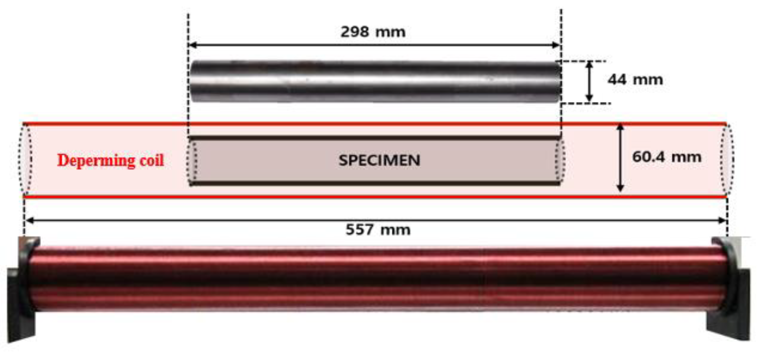
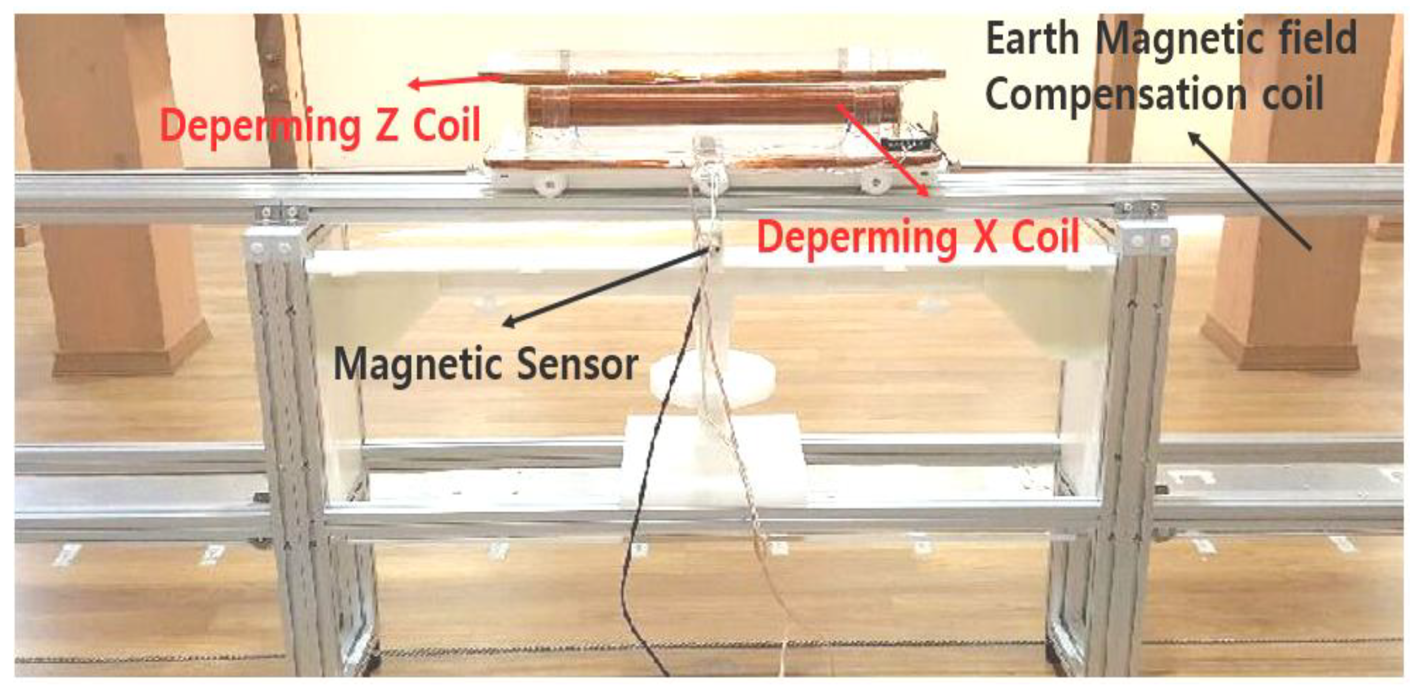
3. Simulation and Experiment Setup

Simulations were performed through a program that combines the Preisach model and Finite Element Method (FEM) to verify the proposed protocol. In addition, experiments were conducted to verify the simulation results. Since the magnitude of the earth’s magnetic field is dependent on the operation areas and the effect of the earth’s magnetic field is compensated by degaussing after demagnetization, for the basic research of the deperming protocol, the effect of the earth’s magnetic field was removed and the experiment was carried out in a Magnetic Treatment Facility.
Figure 8 shows a specimen and the deperming coil used in the simulations and experiments. The length, outer, and inner diameter of the specimen made of the Steel Plate Cold Commercial (SPCC) magnetic material were 298, 44, and 42 mm, respectively. The demagnetizing coil was 557 mm long, 60.4 mm in diameter, and folded in 606 turns. The B-H curve of the SPCC and the Preisach density distribution are shown in Figure 9.

4. Results and Discussion

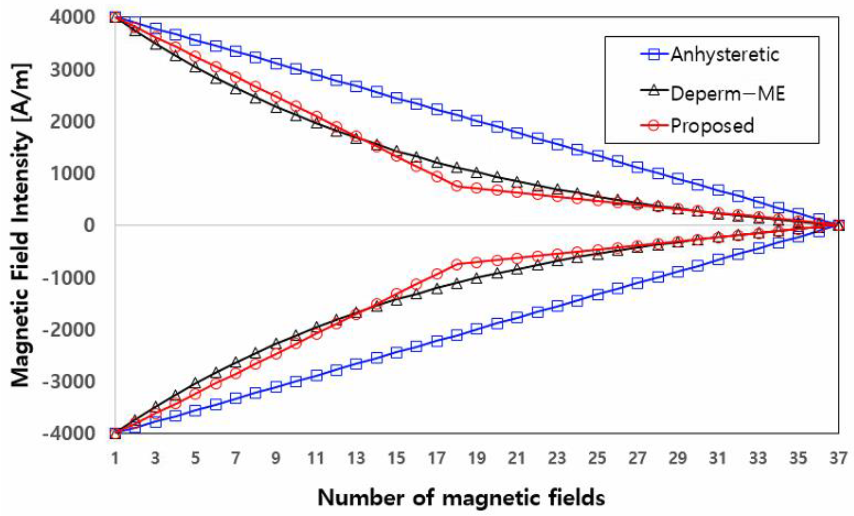
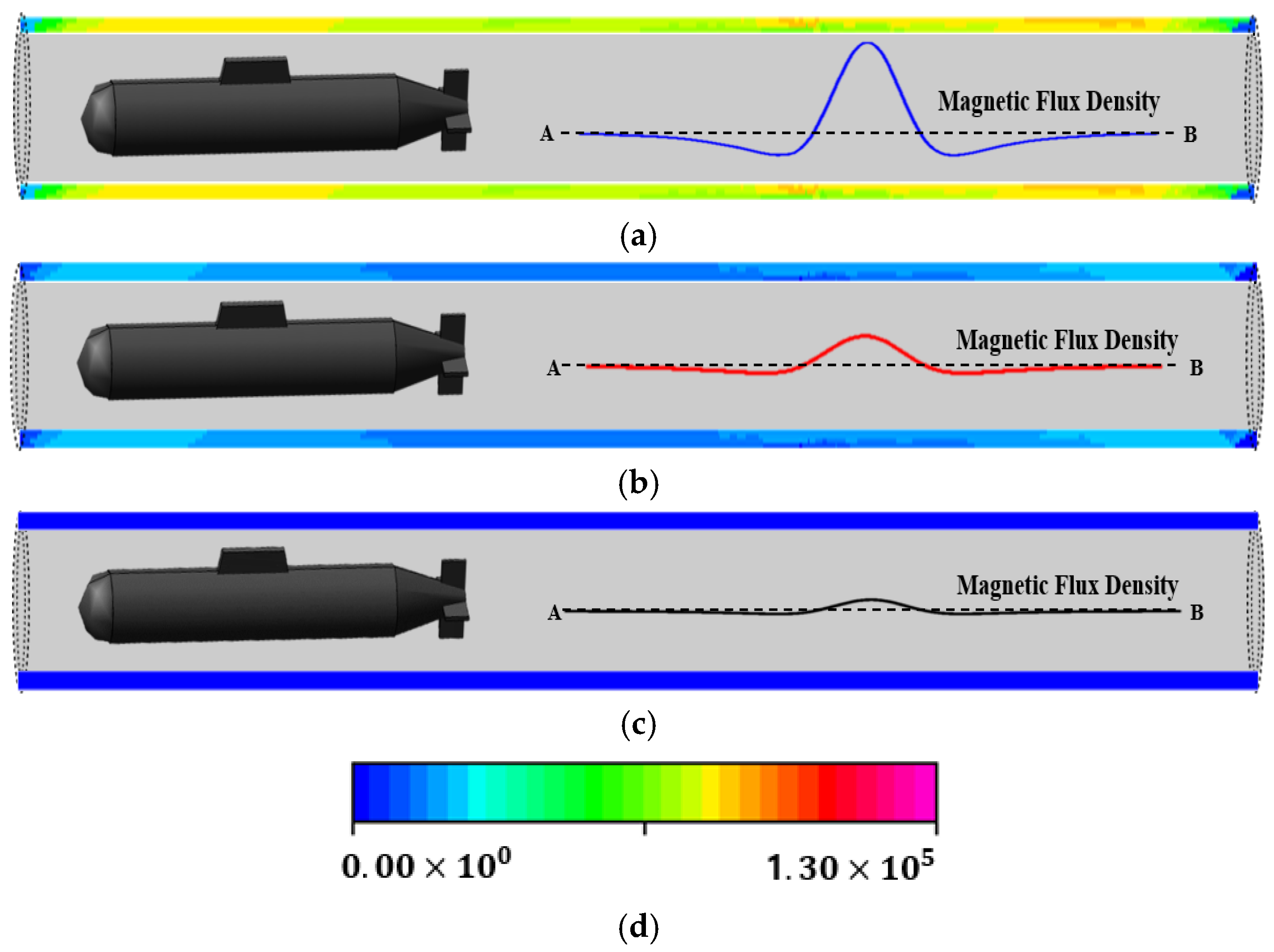
4.1. Simulation Results

Three protocols were applied to the coil for comparison (see Figure 10). The initial and final magnetic fields and the number of the applied magnetic fields were the same. Each magnetic field lasts for 5 s, with a rest period of 3 s. Anhysteretic has a constant decrease of 111.1 A/m. On the other hand, in the proposed protocol, the reduction is 191.2 in Stage 1, and is constantly decreased by 39.5 A/m in Stage 2. The proposed protocol was determined through the process shown in Figure 4.
Figure 11 shows the distribution of the internal magnetization after the demagnetization process performed according to the protocols. After applying the Anhysteretic protocol, a large amount of permanent magnetization remains inside, as shown in Figure 11a. The results obtained through the Deperm-ME protocol were reduced compared to those obtained with the Anhysteretic Deperm protocol. However, as shown in Figure 11c, the internal magnetization after using the proposed protocol was lower than that obtained with the other two protocols. Therefore, the demagnetization performance of the proposed protocol is the best among the protocols.

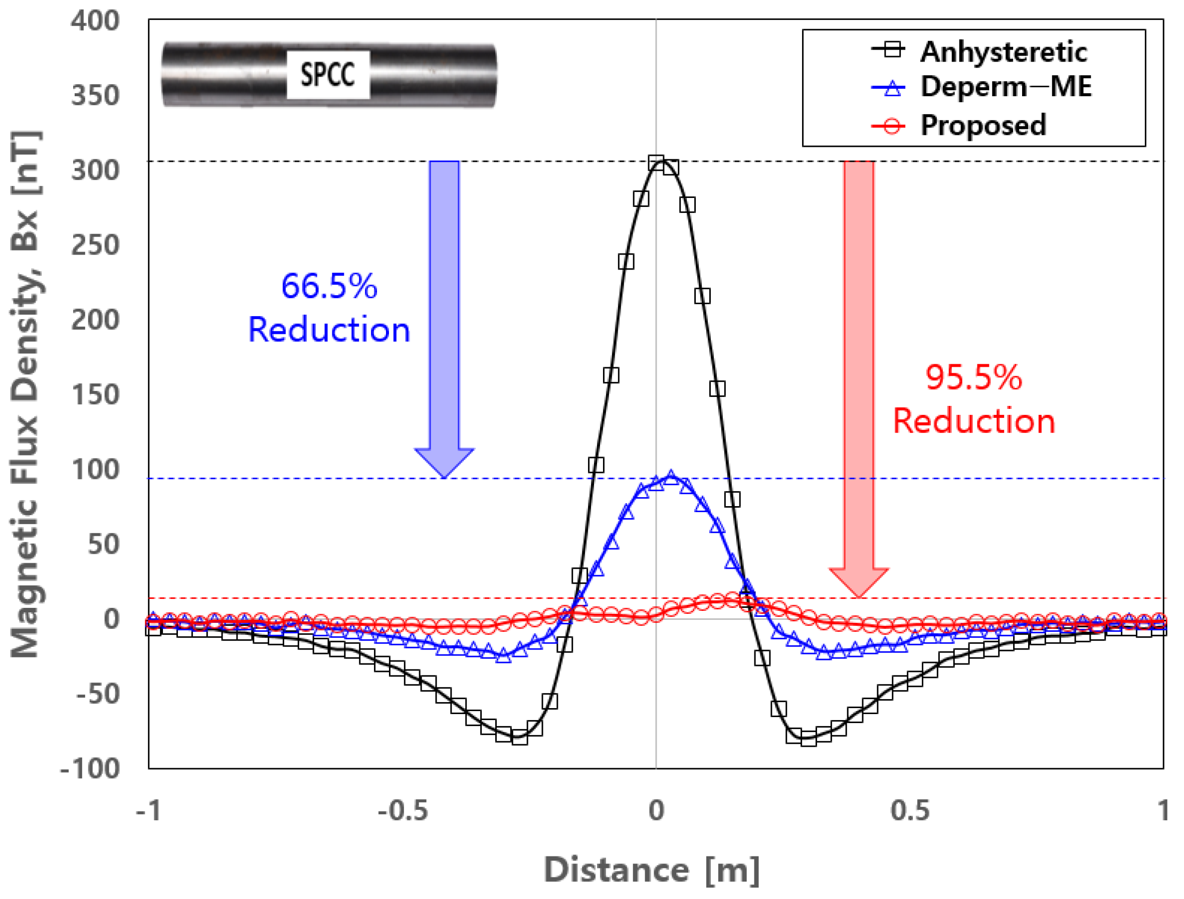
4.2. Experiment Results

Figure 12 shows the experimental setup. A SPCC specimen was placed inside the X coil and three protocols were applied to the X coil. The magnetic flux density was measured with a magnetic sensor (Mag690, Bartington Instruments, Witney, England) to confirm the demagnetization results. The sensor that was positioned 18 cm below it in the vertical direction measured the magnetic flux density while moving the specimen on the aluminum rail. The Z coil was not used in this study since it is used in the Flash-D protocol for submarines. All the devices around the flux-gate magnetic sensor were made of non-magnetic aluminum to minimize the effects of the external magnetic fields.
Figure 13 and Table 1 show the results of the experiment. Since all the protocols used the same number of applied fields, the operating time was the same. When the Deperm-ME protocol was applied, the magnetic flux density was 66.5% lower than that obtained with the Anhysteretic Deperm protocol. The proposed protocol reduced the signal by 95.5%.
Additional experiments were performed to verify whether the proposed protocol could reduce the demagnetization time. Stage 2 is fixed in the proposed protocol, and the number of applied magnetic fields in Stage 1 is reduced by 4 and 8 magnetic fields. Figure 14 and Table 2 show the results of the experiments.
When 4 and 8 magnetic fields were reduced, the flux density increased by 21.4 and 58.4 nT, respectively. As the number of magnetic fields decreased, the signal increased. However, the performance was better than that of Deperm-ME. Furthermore, the demagnetization times were reduced by 11.1% and 22.2%, respectively. Therefore, the proposed protocol has effective performance and reduces the demagnetization time and is easy to control.

5. Conclusions

This paper proposed a novel deperming protocol consisting of two Anhysteretic protocols using the Preisach model. In Stage 1, the previous history was erased through a large initial magnetic field. Due to the low density of the region, unnecessary magnetic fields can be removed. In Stage 2, due to the high density distribution, the performance was improved by drawing the traces uniformly with a slight variation.
The simulations and experiments show that the proposed protocol has better performance than the Anhysteretic and Deperm-ME protocols. In addition, the demagnetization time can be reduced by up to 22% while maintaining excellent performance.

Author Contributions

Conceptualization, S.-H.I. and G.-S.P.; methodology, S.-H.I. and G.-S.P.; data curation, S.-H.I. and H.-Y.L.; writing—original draft preparation, S.-H.I.; writing—review and editing, S.-H.I.; visualization, S.-H.I.; supervision, G.-S.P. All authors have read and agreed to the published version of the manuscript.

Funding

This research was supported by Basic Science Research Program through the National Research Foundation of Korea (NRF) funded by the Ministry of Education (2020R1I1A1A01072534).

Conflicts of Interest

The authors declare no conflict of interest.

References

  1. Modi, A.; Kazi, F. Electromagnetic Signature Reduction of Ferromagnetic Vessels Using Machine Learning Approach. IEEE Trans. Magn. 2019, 55, 6000606. [Google Scholar] [CrossRef]
  2. Norgen, M.; He, S. Exact and explicit solution to a class of degaussing problems. IEEE Trans. Magn. 2000, 36, 308–312. [Google Scholar] [CrossRef]
  3. Raveendra, R.; Varm, A. Design of Degaussing System and Demonstration of Signature Reduction on Ship Model through Laboratory Experiments. Phys. Procedia 2014, 54, 174–179. [Google Scholar]
  4. Tarr, P.B. Method of Measuring Magnetic Effects Due to Eddy Currents. U.S. Patent 4648041A, 3 March 1987. [Google Scholar]
  5. TBynes, M.; Russel, G.J.; Biley, A. Comparison of stepwise demagnetization techniques. IEEE Trans. Magn. 2002, 38, 1753–1758. [Google Scholar]
  6. Wang, R.F.; Li, J.; McConville, W.; Nisoli, C.; Ke, X. Demagnetization protocols for frustrated interacting nanomagnet arrays. J.Appl. Phys. 2007, 101, 9J104. [Google Scholar] [CrossRef] [Green Version]
  7. Ju, H.S.; Chung, H.J.; Im, S.H.; Jeong, D.W.; Kim, J.W.; Lee, H.B.; Park, G.S. Efficient Deperming Protocols Based on the Magnetic Properties in Demagnetization Process. IEEE Trans. Magn. 2015, 51, 7301704. [Google Scholar] [CrossRef]
  8. Ju, H.S.H.W.; Chung, H.J.; Park, G.S. A Study on the Deperm Procols Considering Demagnetizing Field of a Ferromagnetic Material. J. Magn. 2014, 19, 43–48. [Google Scholar] [CrossRef] [Green Version]
  9. Mayergoyz, I.D.; Friedman, G. Generalized Preisach model of hysteresis. IEEE Trans. Magn. 1988, 24, 212–217. [Google Scholar] [CrossRef]
  10. Birsan, M. Simulation of a Ship’s Deperming Process Using the Jiles-Atherton Model. IEEE Trans. Magn. 2021, 57, 7300407. [Google Scholar] [CrossRef]
Figure 1. Schematic view of the demagnetization effects: (a) effect of the permanent magnetization after manufacturing the warship; (b) effect of the demagnetization.
Energies 14 06295 g001
Figure 2. Schematic of Preisach density distribution according to coercivity field and interaction fields on the Preisach plane.
Energies 14 06295 g002
Figure 3. Schematic view of the conventional protocols: (a) Anhysteretic Deperm; (b) Deperm-ME.
Energies 14 06295 g003
Figure 4. Process used to determine the proposed protocol: (a) the process; (b) schematic view of the proposed protocol.
Energies 14 06295 g004
Figure 5. The traces on the Preisach plane following the proposed protocol: (a) the traces on the Preisach plane; (b) magnetization (M)–magnetic field strength (H) curve.
Energies 14 06295 g005
Figure 6. The traces of the Preisach plane in Stage 1 of the proposed protocols: (a) 10 magnetic fields; (b) 8 magnetic fields.
Energies 14 06295 g006
Figure 7. Schematic view of Stage 2 of the proposed protocols: (a) Stage 2 of the proposed protocol; (b) the traces on the Preisach plane.
Energies 14 06295 g007
Figure 8. Model of the demagnetization experiment and simulation.
Energies 14 06295 g008
Figure 9. Magnetic properties of the SPCC: (a) B−H curve; (b) Preisach density distribution on the Preisach plane.
Energies 14 06295 g009
Figure 10. Three types of deperming protocols.
Energies 14 06295 g010
Figure 11. Simulated distribution of the residual magnetization according to the protocols: (a) Anhysteretic Deperm; (b) Deperm-ME; (c) proposed protocol; (d) contour bar.
Energies 14 06295 g011
Figure 12. Sensing system for deperming.
Energies 14 06295 g012
Figure 13. Experimental results of the SPCC following the deperming protocols.
Energies 14 06295 g013
Figure 14. Experimental results obtained with a reduced number of magnetic fields.
Energies 14 06295 g014
Table 1. Measured magnetic flux density of the SPCC following the protocols.
ProtocolsShot NumbersTimeMagnetic Flux Density
(Reduction Rate)
Anhysteretic36288 s304.0 nT
Deperm-ME36288 s94.9 nT (33.5%)
Proposed36288 s12.2 nT (4.5%)
Table 2. Measured results of the SPCC by reducing the demagnetization time.
ProtocolsShot NumbersTime
(Reduction Rate)
Magnetic Flux Density
Deperm-ME36288 s94.9 nT
Proposed36288 s12.2 nT
Reduced 4 shot32256 s
(88.8%)
33.6 nT
Reduced 8 shot28224 s
(77.7%)
70.6 nT
Publisher’s Note: MDPI stays neutral with regard to jurisdictional claims in published maps and institutional affiliations.

