Evaluation of Supervised Learning Models in Predicting Greenhouse Energy Demand and Production for Intelligent and Sustainable Operations

Abstract

Plants need a specific environment to grow and reproduce in fine fettle. Nevertheless, climatic conditions are not stable and can impact their well-being and, consequently, harvest quality. Thus, greenhouse cultivation is one of the suitable agricultural techniques for creating and controlling the inside microclimate to be adequate for plant growth. The relevance of greenhouse control is widely recognized. The prediction of greenhouse variables using artificial intelligence methods is of great interest for intelligent control and the potential reduction in energetic and financial losses. However, the studies carried out in this context are still more or less limited and several machine learning methods have not been sufficiently exploited. The aim of this study is to predict the air conditioning electrical consumption and photovoltaic module electrical production at the smart Agro-Manufacturing Laboratory (SamLab) greenhouse, located in Albenga, north-western Italy. Different supervised machine learning methods were compared, namely, Artificial Neural Networks (ANNs), Gaussian Process Regression (GPR), Support Vector Machine (SVM) and Boosting trees. We evaluated the performance of the models based on three statistical indicators: the coefficient of correlation (R), the normalized root mean square error (nRMSE) and the normalized mean absolute error (nMAE). The results show good agreement between the measured and predicted values for all models, with a correlation coefficient R > 0.9, considering the validation set. The good performance of the models affirms the importance of this approach and that it can be used to further improve greenhouse efficiency through its intelligent control.

1. Introduction

In recent years, the agricultural sector has undergone a clear and rapid evolution. The main objective is to make a compromise between the tremendously increasing food demand and decreasing natural resources while ensuring quality products. Protected agriculture has become more modern and competitive. Nowadays, it adopts innovative and impressive technologies that allow for a rational use of resources and a high yield and quality production. This cultivation technique that has become an integral part of agricultural activity allows for producing different kind of plants throughout the year and during the off season. However, it is an energy-intense cultivation technique with an energy request around 40% of the total production cost [1]. Thus, efficient management can significantly contribute not only to minimizing the energy needs but also to increasing the yield and the quality of the product. The use of intelligent technologies to predict the microclimate inside a greenhouse and/or energy consumption can be of great importance to develop a good energy management strategy and to maintain the required inside air conditions for plant growth.

Currently, the agricultural sector faces a real revolution. The advent of technologies and the implementation of artificial intelligence (AI) play a key role in this revolution and have taken the agriculture framework to an advanced level [2]. Artificial intelligence (AI) can lead to real-time monitoring and decision making, which can be of considerable interest to further improve and develop this sector. Substantial research has been devoted to this target. Jha et al. [3] presented a comprehensive review of the present state of automation in agriculture and discussed the applications of Artificial Neural Networks (ANNs), machine learning (ML) and the Internet of Things (IoT) for precision farming. In another review paper, Patrício and Riederb [4] evaluated the approaches and the issues of computer vision and artificial intelligence applied to precision crops grain agriculture. Pantazi et al. [5] described in exhaustive manner different artificial intelligence methods and their applicability in precision farming. Artificial intelligence (AI) can be applied in protected agriculture in many ways, such as to maintain an adapted microclimate to the plant growth, to optimize the irrigation process, to properly apply pesticides and herbicides or to optimize the energy consumption.

To predict the agricultural greenhouses variables, different machine learning (ML) methods can be used. Artificial Neural Networks (ANNs) have been largely used to this purpose. Pahlavan et al. [6] analyzed ANNs with different architectures to predict the yield of basil greenhouses’ production in Isfahan province, Iran. The energy equivalent of human labor, diesel fuel, chemical fertilizers, farm yard manure, chemicals, electricity and transportation were fixed as inputs and the basil yield as output. In [6], a multilayer perceptron ANN with a 7-20-20-1 structure was considered as the best model with a coefficient of determination of 0.976, a root mean square error of 0.046 and a mean absolute error of 0.035. To model the greenhouse inner air humidity under the climatic conditions of northern China, He et al. [7] proposed an ANN model using a back-propagation (BP) training learning method based on the principal component analysis (PCA) method (to simplify network structure and the data samples). In their study, the accuracy of the model was evaluated using the coefficient of determination, and a value of 0.8842 was obtained in the validating phase. In another study, Uchida Frausto and Pieters [8] proposed an ANN with a vector containing the regressors of an auto-regressive model with exogenous variables (ARX). The proposed model was used to predict the air temperature inside a greenhouse based on the external air temperature and humidity, global solar radiation and sky cloudiness. Their findings show the importance of the selection of an adequate number of neurons in the hidden layer, given their impact on the prediction accuracy. According to the authors, an agreement up to 75% was found when using 20 neurons in the hidden layer, and it dropped to around 40% when using eight neurons in the hidden layer.

Furthermore, other methods can be used in predicting greenhouses variables. Taki et al. [9] studied the feasibility of controlling greenhouse climate conditions and energy consumption for a polyethylene greenhouse in the climatic conditions of Isfahan province, Iran. In their study, a comparison of ANN (multilayer perceptron (MLP) with radial basis function (RBF)) and Support Vector Machine (SVM) methods was conducted. The results showed that the RBF neural network model is more accurate in estimating the parameters inside the greenhouse and the energy exchange, with a range of root mean square error of about 0.07–0.12 °C. In another work, Yu et al. [10] predicted the inside air temperature of a Chinese solar greenhouse using a Least Squares Support Vector Machine (LSSVM) optimized by the improved particle swarm optimization algorithm (IPSO). The LSSVM model showed suitable accuracy compared to standard SVM and back propagation ANN (BP-ANN), with a lower mean square error of about 0.0281. Zou et al. [11] predicted the inside air temperature and humidity of a solar greenhouse in the Institution Vegetable and Fruit of Chinese Academy of Agricultural Sciences using the convex bidirectional extreme learning machine (CB-ELM) method. This method showed the highest accuracy (root mean square error of about 1.4409 °C and 2.4988% for temperature and relative humidity, respectively) compared to Bidirectional Extreme Learning Machine (B-ELM), Back Propagation Neural Network (BPNN), Support Vector Machine (SVM) and Radial Basis Function (RBF).

The use of machine learning methods for predicting greenhouse variables is of great interest to develop intelligent management strategies and reduce potential energetic and financial losses. Moreover, several machine learning methods have not been sufficiently exploited. This study focuses on predicting the air conditioning electrical consumption and the photovoltaic module electrical production that will make it possible to have a preliminary idea of the energy needs and resources of the greenhouse for a better management, and that can also help reduce some financial costs related to measurement and monitoring instrumentation. The prediction is performed using different supervised machine learning algorithms, namely, Artificial Neural Networks (ANN), Gaussian Process Regression (GPR), Support Vector Machine (SVM) and Boosting. We evaluated and compared the performance of the models based on three statistical indicators: the coefficient of correlation (R), the normalized mean absolute error (nMAE) and the normalized root mean square error (nRMSE).

2. Materials and Methods

2.1. Data Sets

In this study, the datasets used to build the studied models were provided by the monitoring system of the Smart Agro-Manufacturing Laboratory (SamLab) greenhouse [12]. This high-efficiency greenhouse is located in Albenga, Italy, and occupies an area of 151.47 m² with an even span shape (15.30 m length, 9.9 m width, 3.5 m eave height and 5.6 m roof-top height) and a glass envelop with a galvanized steel structure and aluminum frame (Figure 1). The greenhouse is equipped with passive technologies (operable windows and shading/reflecting system) and renewable energy systems (semi-transparent PV panels and a ground coupled heat pump, GCHP). A more detailed description of the greenhouse is presented in a previous investigation by the authors [13].

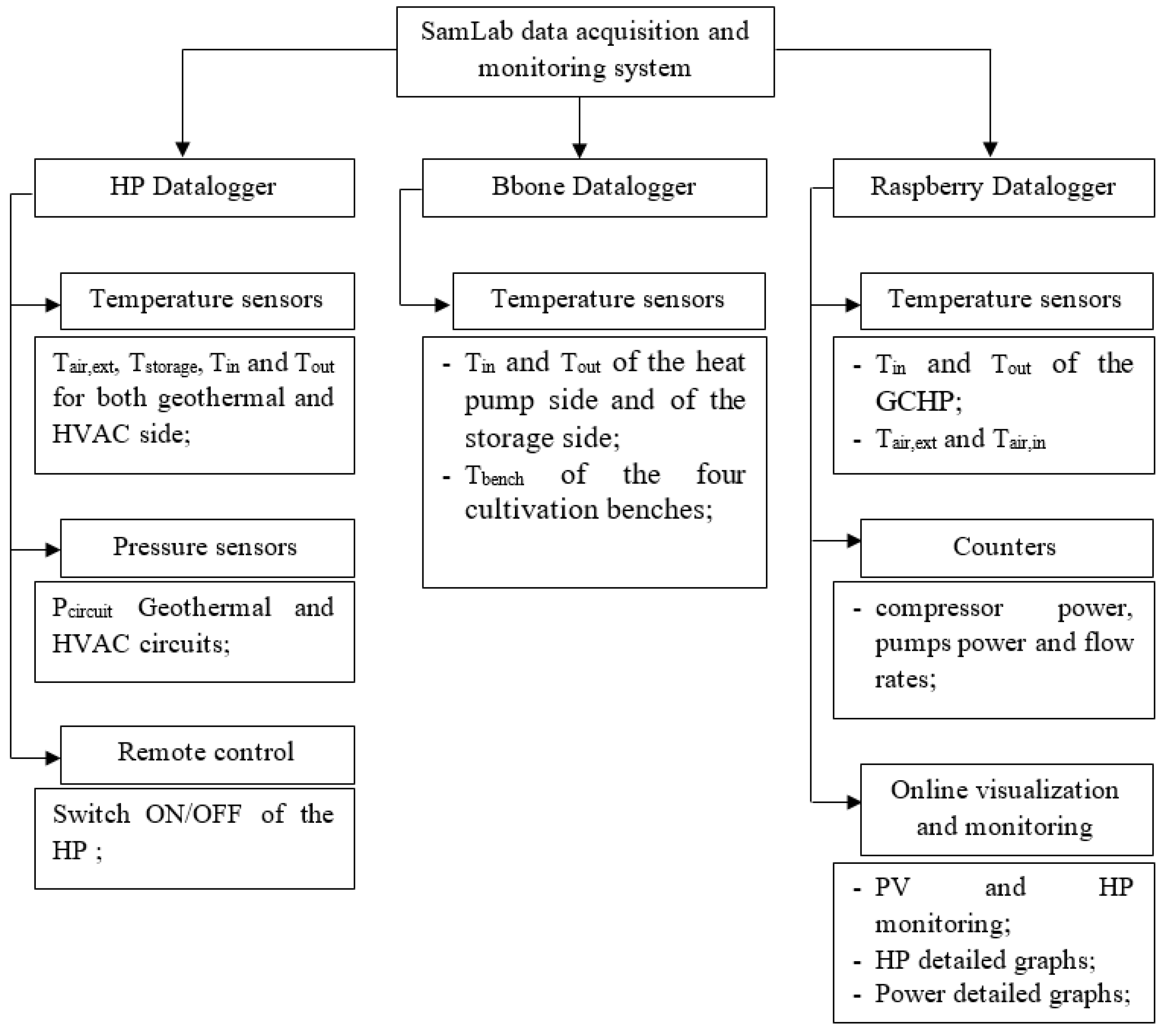
2.2. Data Acquisition

The SamLab greenhouse is equipped with a complete data acquisition and monitoring system that measures and records different parameters related to the greenhouse systems and the inside climatic conditions. Many pressure, temperature and mass flow rate sensors allow acquiring a huge amount of hourly and sub hourly data. This data acquisition system is composed of different subsystems: the EcoForest Heat Pump (HP) Datalogger (webserver inside the HP), the Bbone Datalogger and the Raspberry Datalogger, as presented in Figure 2. Moreover, external temperature and solar radiation, related to the selected time periods (March and mid-August to mid-September 2020), are used to train and validate the models. The data for the analyzed location (i.e., Albenga) are partially measured on site (temperature) and partially deduced from the “Liguria Region Agency for the Environment” webpage [14] (solar irradiance).

2.3. Description of the Models

The main goal of this study is to compare the performance of four methods in predicting the air conditioning electrical consumption and PV module electrical production. The following methods were attempted: ANN, GPR, SVM and Boosting. To reach this goal, the present study follows 3 steps, summarized as follow: random split of the dataset (70% for training and 30% for validation), implementation of the four different models, optimization of the chosen models hyperparameters to improve their performance and comparison of the models’ performance in terms of their statistical indicators (Section 2.4).

During the training phase, both input and output (training dataset) data are provided to the models so the models could learn from them. The validation dataset is inaccessible until the models are completely trained. The inputs of the validation dataset are used to predict the desired outputs, and they are compared to the actual outputs.

The models’ hyperparameters, as parameters allowing for controlling the learning process, strongly affect their performance. In this study, for GPR, SVM and Boosting tree models, the selection of the optimal parameters was carried out by automatically trying different hyperparameter combinations based on an optimization scheme that aims to minimize the mean square error (MSE) of the model and returns the model using optimized hyperparameters. The optimal parameters depend on the predicted parameters.

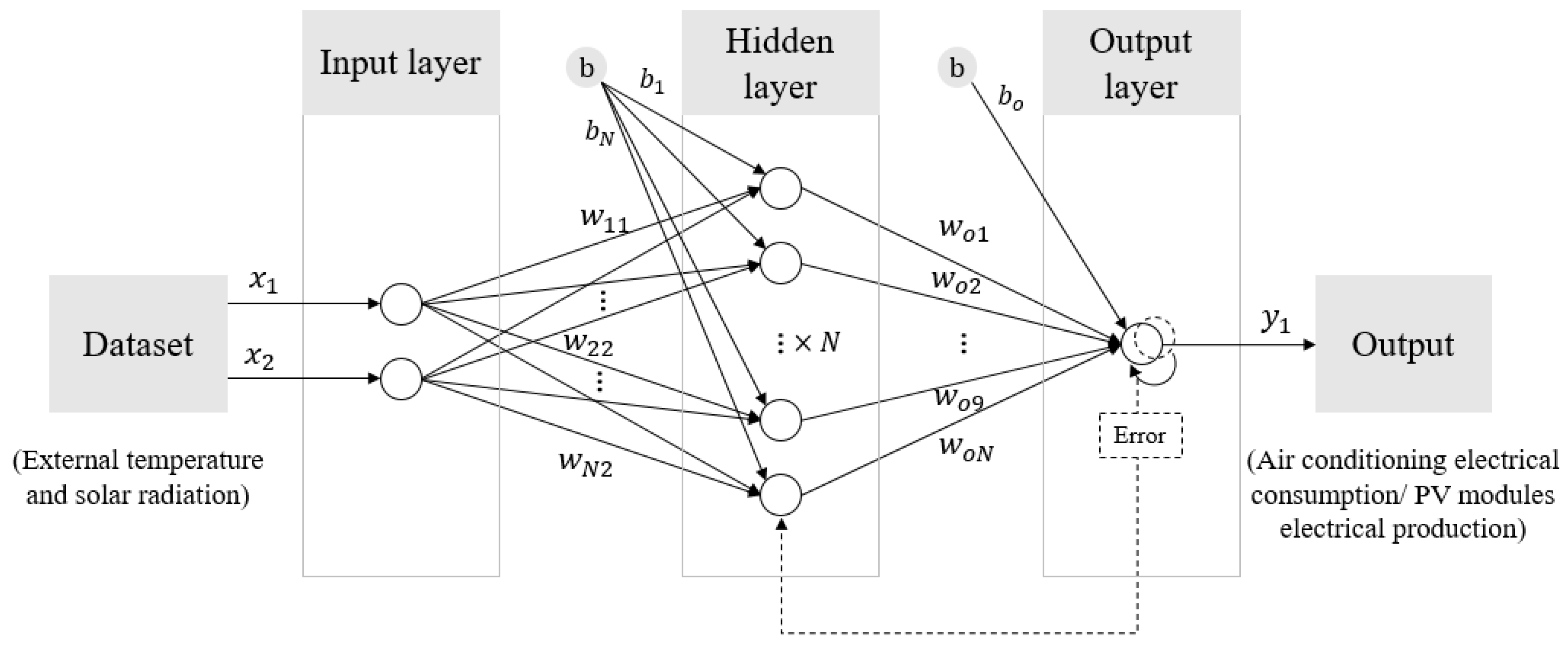
2.3.1. Artificial Neural Networks, ANNs

Artificial Neural Networks (ANNs) are powerful methods that have shown their ability to solve complex nonlinear problems and determine the relationship between inputs and outputs. The fundamentals of ANNs were inspired by the structure of the human brain system [15].

In this study, a “back propagation” multi-layer perceptron neural network is used. The network architecture (2-10-1) is composed of one input layer with two neurons (external temperature and global solar radiation), one hidden layer with ten neurons and one output layer with one neuron (air conditioning electrical consumption or PV module production), as presented in Figure 3. The selected activation function is the hyperbolic tangent sigmoid function (Equation (2)).

$$y=w_{oh}a\left(w_{hi}x+b_h\right)+b_o$$

(1)

$$a\left(w_{hi}x+b_h\right)=\frac{2}{1+e^{-2\left(w_{hi}x+b_h\right)}}-1$$

(2)

where $w_{hi}$ is the weights the matrix of the connections between the inputs and the hidden neurons, $w_{oh}$ is the weights vector of the connections between the hidden and the output neurons, $b_h$ is the vector of biases of the hidden neurons and $b_o$ is the bias of the output neuron.

2.3.2. Gaussian Process Regression, GPR

Gaussian Process Regression is a powerful supervised machine learning method that showed its ability for learning and accurately predicting from a small dataset. It is an application of the Gaussian process to solve regression problems [16], defined as a collection of random variables in a way that any subset of them is jointly Gaussian. Furthermore, the Gaussian process could represent the distribution over a random function $f(x)$ evaluated at any specific input $x\in {ℝ}^d$. As presented in Equation (3) [17], the Gaussian process is specified by the mean function $m\left(x\right)$ (Equation (4) [17]) and the kernel function, or the so-called covariance function $k\left(x,x^{\prime }\right)$ (Equation (5) [17]).

$$f\left(x\right)\sim GP\left(m\left(x\right),k\left(x,x^{\prime }\right)\right)$$

(3)

$$m\left(x\right)=\mathrm{E}\left|f\left(x\right)\right|$$

(4)

$$k\left(x,x^{\prime }\right)=\mathrm{E}\left[\left(f\left(x\right)-m\left(x\right)\right)\left(f\left(x^{\prime }\right)-m\left(x^{\prime }\right)\right)\right]=\mathrm{cov}\left(f\left(x\right),f\left(x^{\prime }\right)\right)$$

(5)

Considering that ${\left\{x_i,y_i\right\}}_{i=1}^{i=N}\in \left({ℝ}^d,ℝ\right)$ is the training dataset and ${\left\{x_{i,*}\right\}}_{i=1}^{i=N}\in {ℝ}^d$ is the validation dataset, the distribution of Gaussian process functions is given in Equation (6) [17].

$$\left(\begin{array}{c}f\left(x\right)\\ f\left(x_{*}\right)\end{array}\right)\sim N\left(\left(\begin{array}{c}m\left(x\right)\\ m\left(x_{*}\right)\end{array}\right),\left(\begin{array}{cc}\begin{array}{c}k\left(x,x\right)+{\sigma }^{2}I\\ k\left(x_{*},x\right)\end{array}& \begin{array}{c}k\left(x,x_{*}\right)\\ k\left(x_{*},x_{*}\right)\end{array}\end{array}\right)\right)$$

(6)

where ${\sigma }^2$ is a GP hyper-parameter, indicating the covariance noise.

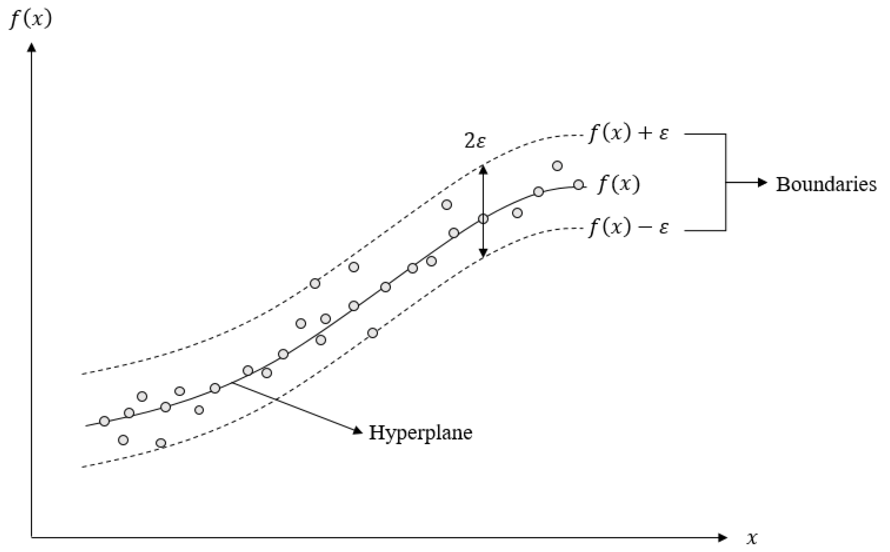
2.3.3. Support Vector Machine SVM

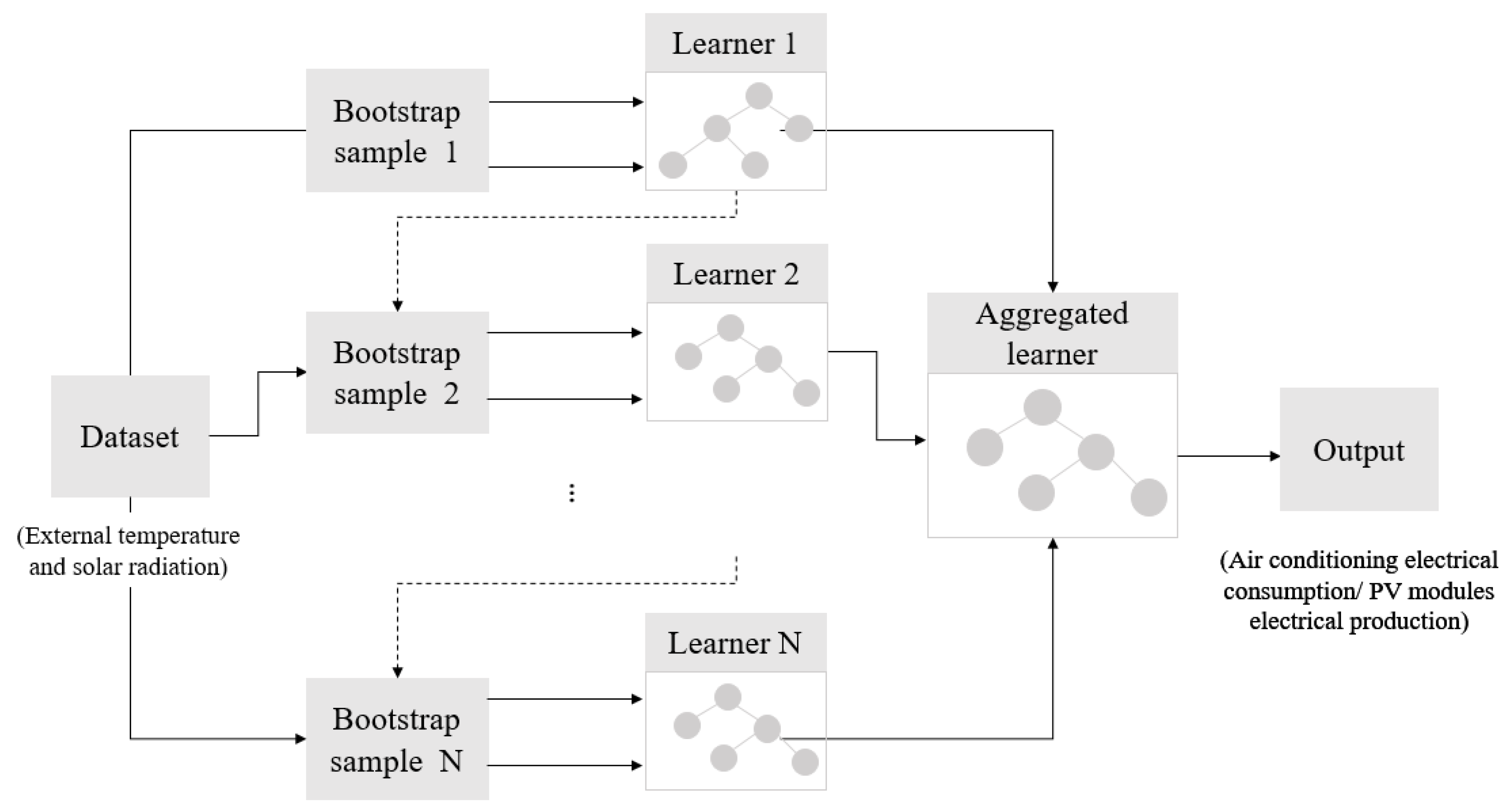
The Support Vector Machine regression method is derived from the early support vector machine developed to solve classification problems [18]. This method seeks a function that roughly maps the variation of the actual output parameters from the input parameters based on a training sample. The best function is the hyperplane that gathers a maximum number of points (Figure 4). Then, the model becomes able to predict the variation of the output parameters from a new dataset containing only the input parameters.

Considering that ${\left\{x_i,y_i\right\}}_{i=1}^{i=N}\in \left({ℝ}^d,ℝ\right)$ is the training dataset and ${\left\{x_{i,*}\right\}}_{i=1}^{i=N}\in {ℝ}^d$ is the validation dataset, the equation of the hyperplane is presented in Equation (7) [19]. $w$ and $b$ are the model parameters.

$$f\left(x\right)=\left(w,x\right)+b$$

(7)

where $w$ is a vector and $b$ is a scalar. Support vector regression aims to find the best hyperplane characterized by $w^{*}$ and $b^{*}$ that minimize the overall gap between $f$ and $y_i$ and giving a better fitting model (Equation (8) [19]).

$$\left(w^{*},b^{*}\right)=\arg {\min }_{w,b}{\displaystyle \sum _{i=1}^n\left(y_i-\left(w,x_i\right)-b^2\right)}$$

(8)

2.3.4. Boosting

Boosting is one of the competitive ensemble methods based on gathering multiple learners into an aggregate predictor that undoubtedly expands the domain of solutions [20]. Furthermore, each learner is individually different from the other, making it possible to extract different relationships from a given dataset, which will yield much better results than a single individual predictor. Thus, it leads to a long training time (long simulation time). The particularity of Boosting compared to the other techniques of ensemble methods is that each learner seeks to correct the weaknesses of the previous one by an iterative approach, reducing the bias, as presented in Figure 5.

Considering that ${\left\{x_i,y_i\right\}}_{i=1}^{i=N}\in \left({ℝ}^d,ℝ\right)$ is the training dataset and ${\left\{x_{i,*}\right\}}_{i=1}^{i=N}\in {ℝ}^d$ is the validation dataset, $M$ is the regression trees model and $e$ is the residual in Equations (9) and (10) [21].

$$y_i=M_1\left(x_i\right)+{\epsilon }_{1i}$$

(9)

$$e_{1i}=y_i-M_1\left(x_i\right)$$

(10)

The residual is modeled with a second model $M_2$ and then associated to the previous one. The goal is to compensate for the deficiency of $M_1$ for a better prediction, as presented in Equations (11) and (12) [21]. The same applies for the residual $e_2$.

$$e_{1i}=M_2\left(x_i\right)+{\epsilon }_{2i}$$

(11)

$$y_i^{\prime }=M_1\left(x_i\right)+M_2\left(x_i\right)$$

(12)

2.4. Performance Analysis

In order to assess the performance of the studied methods in predicting the desired outputs, three of the statistical indicators widely used in the literature are employed to compare the predicted and measured values: the coefficient of correlation ($R$), the normalized root mean square error ($nRMSE$) and the normalized mean absolute error ($nMAE$); these indicators are calculated based on Equations (13), (14) and (15) [22], respectively. Normalized values of MAE and RMSE are used to prevent the dataset scale dependency [23].

$$R=\frac{{\displaystyle \sum _{i=1}^n}\left(M_i-\overline{M}\right)\cdot \left(P_i-\overline{P}\right)}{\sqrt{\left[{\displaystyle \sum _{i=1}^n}{\left(M_i-\overline{M}\right)}^2\right]\cdot \left[{\displaystyle \sum _{i=1}^n}{\left(P_i-\overline{P}\right)}^2\right]}}\cdot 100$$

(13)

$$nRMSE=\frac{\sqrt{\raisebox{1ex}{$1$}\!\left/ \!\raisebox{-1ex}{$n$}\right.{\displaystyle \sum _{i=1}^n}{\left(P_i-M_i\right)}^2}}{\overline{M}}\cdot 100$$

(14)

$$nMAE=\frac{\raisebox{1ex}{$1$}\!\left/ \!\raisebox{-1ex}{$n$}\right.{\displaystyle \sum _{i=1}^n}\left|P_i-M_i\right|}{\overline{M}}\cdot 100$$

(15)

where $P_i$ and $M_i$ are the $i\mathrm{th}$ predicted and measured values, and $\overline{P}$ and $\overline{M}$ are their mean values, respectively. The coefficient of correlation ($R$) measures the strength of the relationship between predicted and measured values; when the paces of the curves are similar, the correlation coefficient $R$ is close to one. The normalized root mean square error ($nRMSE$) allows for evaluating the dispersion of the predicted values in respect to the measured ones. Finally, the normalized mean absolute error ($nMAE$) allows for measuring the absolute error between the predicted and measured values, which could help evaluate the model’s accuracy. When the values of both $nRMSE$ and $nMAE$ are close to zero, the models are considered better.

3. Results and Discussions

In this section, the main results obtained in predicting the air conditioning electrical consumption and PV module electrical production are presented. The performance of each model in predicting the outputs (air conditioning electrical consumption, PV module electrical production) are evaluated for each studied machine learning method, namely, ANN, GPR, SVM and Boosting. For all models, the dataset is randomly split into two subsets using the “Holdout” method. The first one (70%) has been used to train the model and the second one (30%) has been used to validate the model.

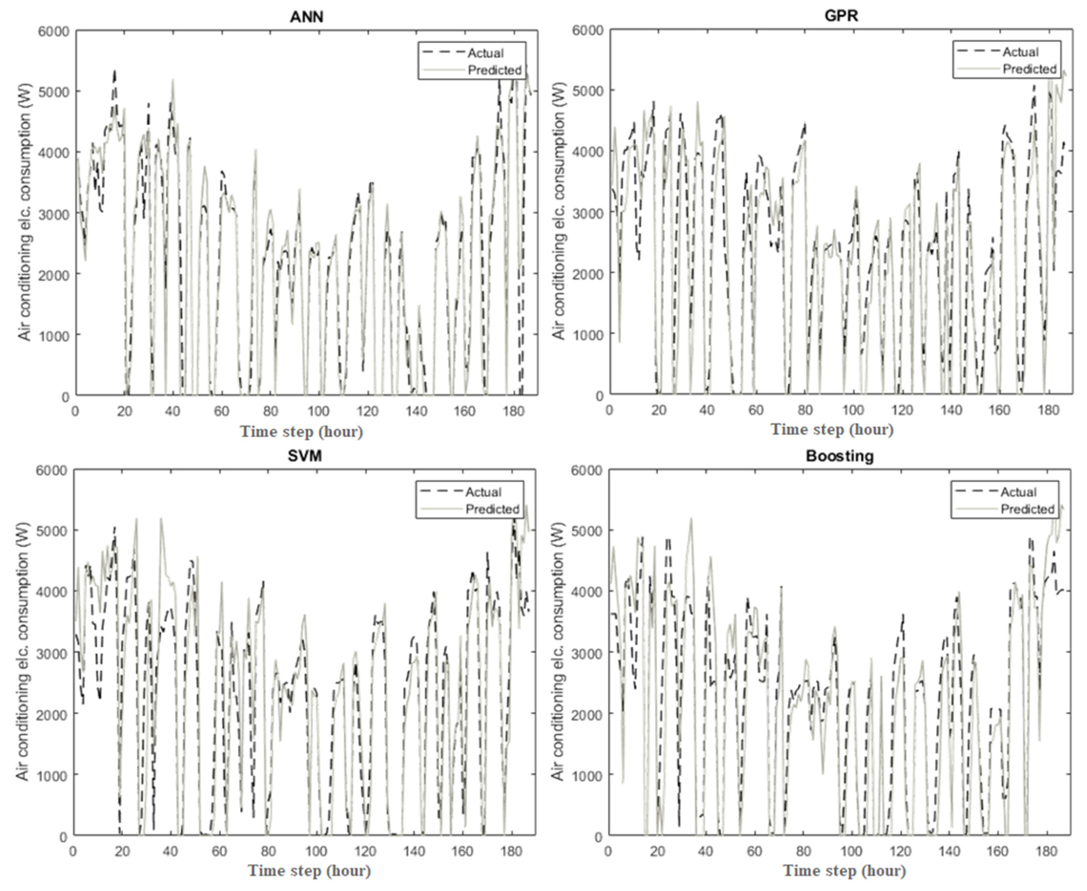
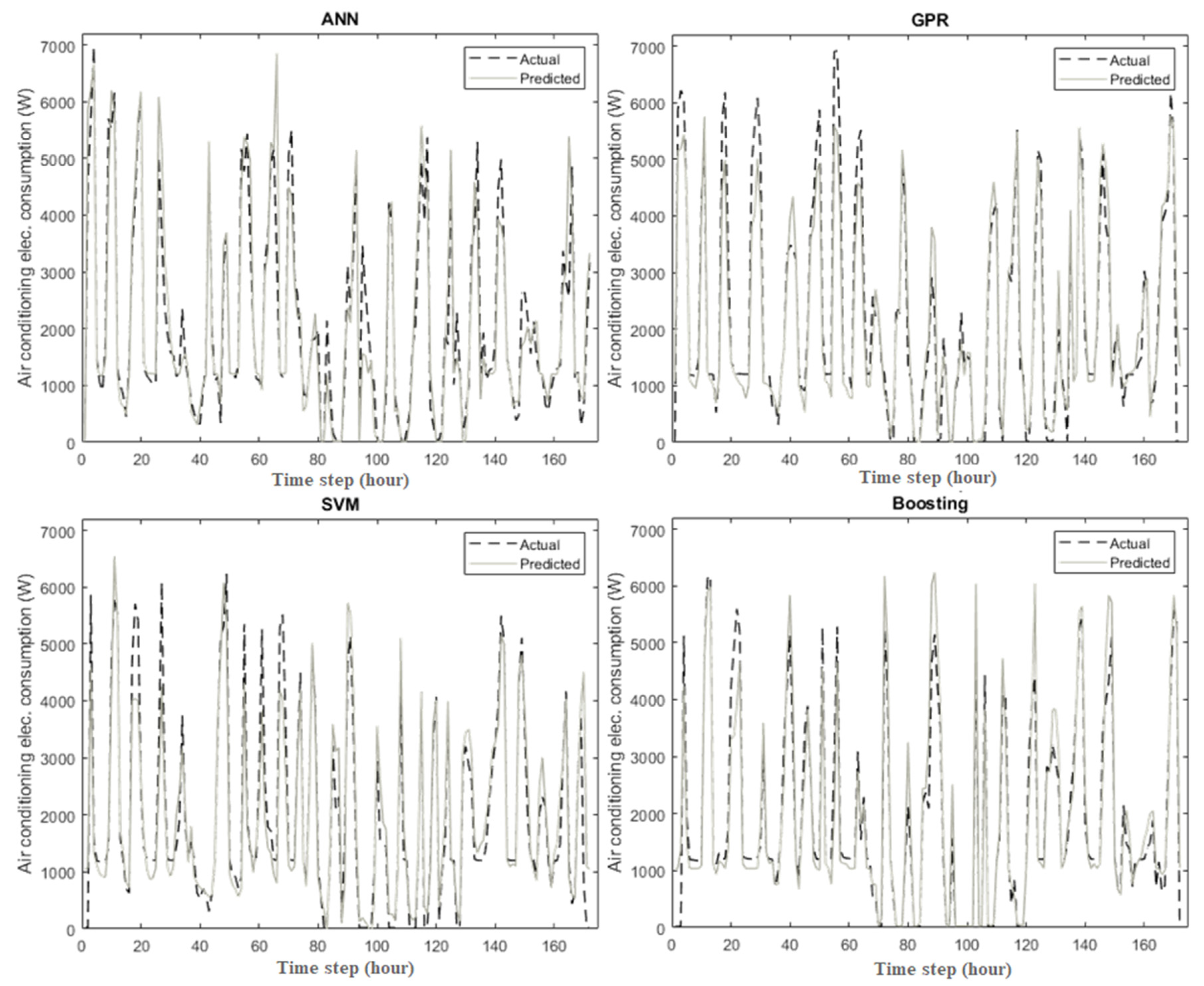
3.1. Prediction of the Air Conditioning Electrical Consumption

Figure 6 and Figure 7 present the curves of variation of the air conditioning electrical consumption, during the month of March and from mid-August to mid-September, respectively, using the four studied machine learning methods. The graphs show that the predicted values have good agreement with the measured ones, with coefficients of correlation in the validation phase and for the month of March of about 92.46% for ANN, 91.57% for GPR, 90.76% for SVM and 91.17% for Boosting. For the period from mid-August to mid-September, the coefficients of correlation are around 94.01%, 96.21%, 94.05% and 95.96% for ANN, GPR, SVM and Boosting, respectively.

The results obtained for the period from mid-August to mid-September are much better than those obtained for the month of March. This could be explained by the fact that during summer days, the external temperature and solar radiation (inputs of the models) are the main parameters influencing the microclimate inside a greenhouse and could be sufficient in predicting its air conditioning electrical consumption. On the contrary, during the month of March, other climatic parameters are more intensive and can influence the greenhouse microclimate, e.g., wind, precipitation and sky cloudiness. GPR outperforms all evaluated models in predicting the air conditioning electrical consumption in the period from mid-August to mid-September. For the month of March, the ANN model slightly outperforms the other models.

Table 1. The models’ performance in predicting the air conditioning electrical consumption (March, mid-August to mid-September).

Output	Period	Model		Training			Validation
				$\mathit{R}$ (%)	$\mathit{n}\mathit{R}\mathit{M}\mathit{S}\mathit{E}(\%)$	$\mathit{n}\mathit{M}\mathit{A}\mathit{E}(\%)$	$\mathit{R}$ (%)	$\mathit{n}\mathit{R}\mathit{M}\mathit{S}\mathit{E}(\%)$	$\mathit{n}\mathit{M}\mathit{A}\mathit{E}(\%)$
Air conditioning electrical consumption	March 2020	ANN	2-10-1	97.8712	18.8831	10.8624	92.4610	12.9642	5.321
		GPR	$\sigma =1.5$	91.2684	24.4969	15.0304	91.5676	15.7289	6.4811
		SVM	$\epsilon =6.35$	91.0673	24.0926	13.8872	90.7590	15.4800	6.1483
		Boosting	36 learners	91.6594	22.6429	13.6338	91.1679	16.8750	6.4712
	Mid-August/Mid-September 2020	ANN	2-10-1	97.6209	24.9683	13.6470	95.0121	15.0257	5.3083
		GPR	$\sigma =4.7$	96.3606	19.6298	10.5916	96.2057	12.8562	4.9058
		SVM	$\epsilon =2.49$	95.5177	22.3990	13.0860	94.0457	15.4998	5.4185
		Boosting	10 learners	97.7934	15.3439	8.6856	95.9600	13.8336	4.9534

summarizes the statistical indicators ($R$, $nRMSE$ and $nMAE$) of the models in predicting the air conditioning electrical consumption in the month of March and from mid-August to mid-September.

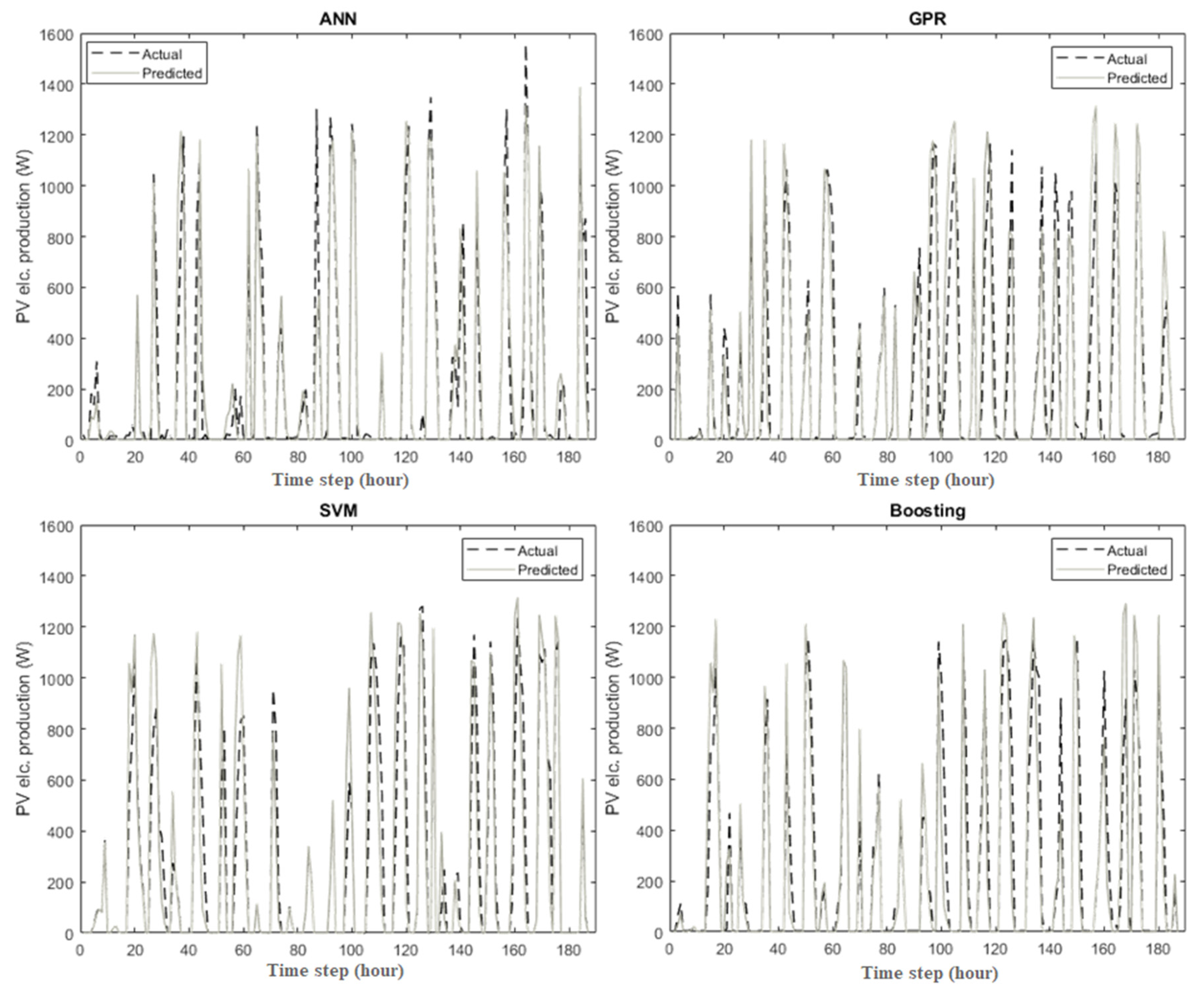
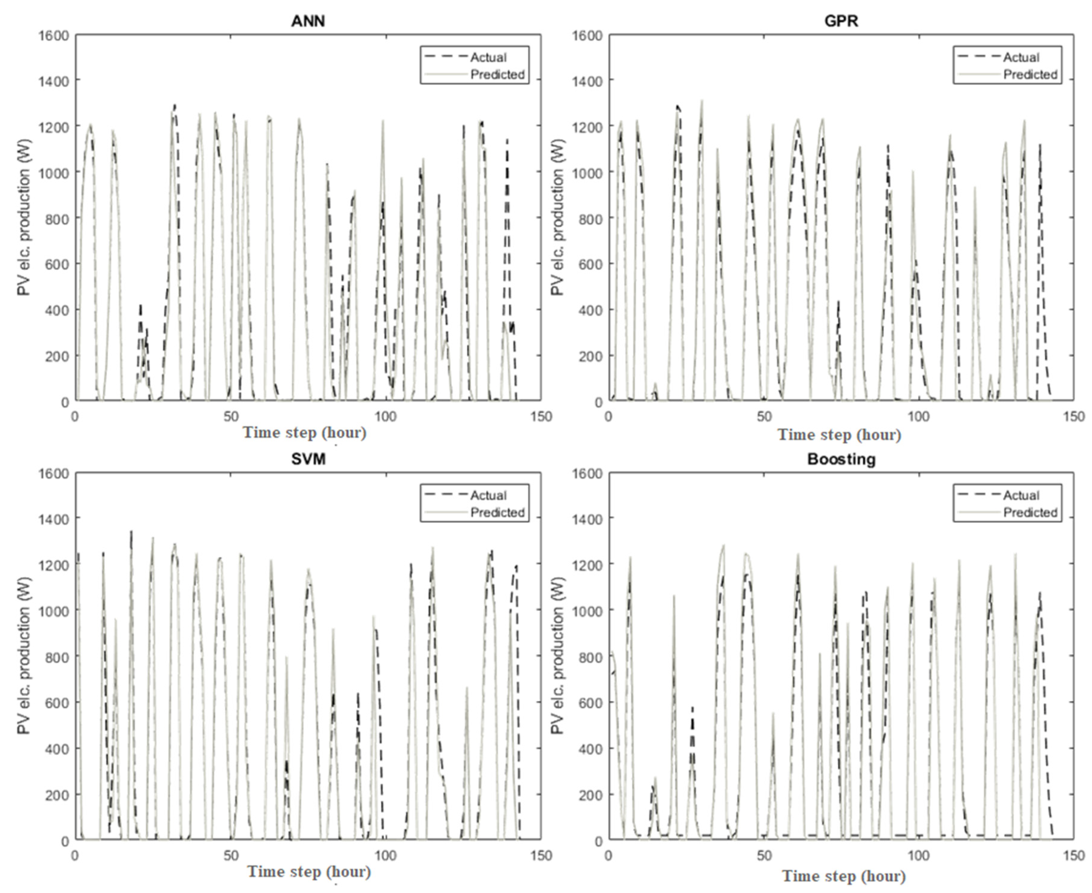
3.2. Prediction of PV Module Electrical Production

Figure 8 and Figure 9 present the curves of variation of the PV module electrical production, during the month of March and from mid-August to mid-September, respectively, using the four studied machine learning methods. The graphs show that the predicted values have a good agreement with the measured ones, with coefficients of correlation in the validation phase and for the month of March of about 96.12% for ANN, 92.38% for GPR, 91.29% for SVM and 91.88% for Boosting. For the period from mid-August to mid-September the coefficients of correlation are around 96.33%, 94.21%, 93.55% and 94.13% for ANN, GPR, SVM and Boosting, respectively.

Comparing the coefficients of correlation and considering the validation sets, the ANN model outperforms the studied models in predicting the PV module electrical production, in both periods, especially for the month of March. The ANN model is followed by GPR, then Boosting trees and finally, the SVM method. As for the prediction of the air conditioning electrical consumption, the models have better performance in predicting the PV module electrical production during the period of mid-August to mid-September; the same explanation as stated previously could be provided.

Table 2. The models’ performance in predicting PV module electrical production (March, mid-August to mid-September).

Output	Period	Model		Training			Validation
				$\mathit{R}$ (%)	$\mathit{n}\mathit{R}\mathit{M}\mathit{S}\mathit{E}(\%)$	$\mathit{n}\mathit{M}\mathit{A}\mathit{E}(\%)$	$\mathit{R}$ (%)	$\mathit{n}\mathit{R}\mathit{M}\mathit{S}\mathit{E}(\%)$	$\mathit{n}\mathit{M}\mathit{A}\mathit{E}(\%)$
PV module electrical production	March 2020	ANN	2-10-1	97.3864	33.1328	20.9550	96.3285	22.0497	10.0231
		GPR	$\sigma =3.97$	92.6129	42.7174	21.9205	92.3836	21.4978	9.4679
		SVM	$\epsilon =0.7150$	92.7159	42.7893	20.7340	91.2903	23.3442	9.3637
		Boosting	39 learners	94.1176	35.9266	19.7293	91.8845	24.7175	9.8309
	Mid-August/Mid-September 2020	ANN	2-10-1	97.6136	30.0094	16.1551	96.1150	20.2251	8.6132
		GPR	$\sigma =4.41$	95.0153	24.9565	13.9918	94.2151	13.6115	6.1538
		SVM	$\epsilon =7.65$	95.3025	23.6884	12.2957	93.5519	17.3420	5.5604
		Boosting	36 learners	95.6063	21.5596	13.7941	94.1332	16.1418	7.1238

presents the models’ performance in predicting the PV module electrical production in the month of March and from mid-August to mid-September.

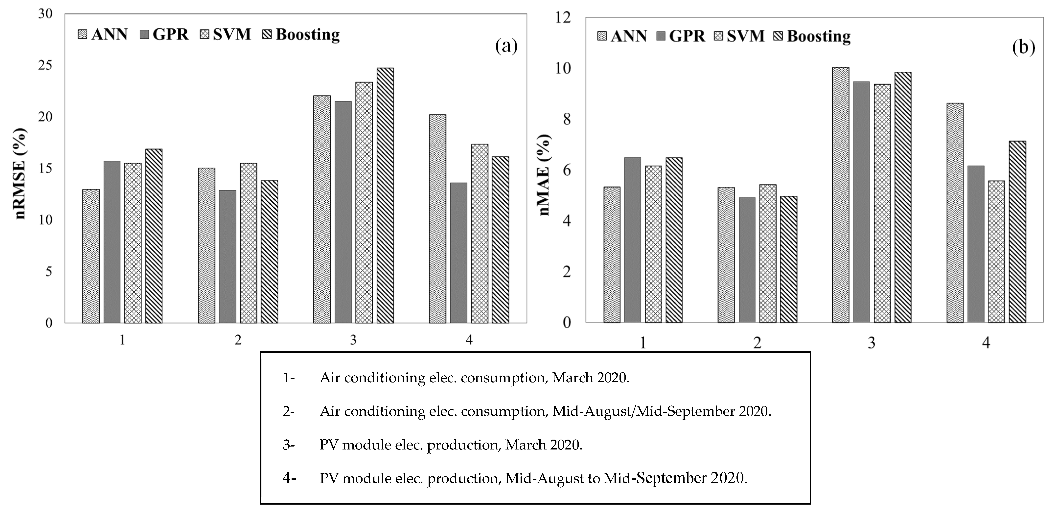
3.3. Comparison and Analysis

The normalized root mean square error (nRMSE) is also a good statistical indicator in evaluating the models’ performance. In this study, the nRMSE varies between 12.86% (prediction of the air conditioning electrical consumption in the period from mid-August to mid-September using the GPR model) to 24.72% (prediction of the PV module electrical production in the month of March using the Boosting trees method), as presented in Figure 10a. According to several studies [23,24,25], the selected models have acceptable to good performances ($10\%<nRMSE<30\%$). The nRMSE values varies from 12.96% to 22.05% for the ANN, from 12.86% to 21.50% for the GPR, from 15.48% to 23.34% for the SVM and from 13.83% to 24.72% for the Boosting trees method.

Figure 10b shows the variation of the nMAE in predicting the air conditioning electrical consumption and the PV module electrical production using the four machine learning methods (ANN, GPR, SVM, Boosting). The values vary from 4.91% (prediction of air conditioning electrical consumption in the period of mid-August to mid-September using the GPR method) to 10.02% (prediction of PV module electrical production during the Month of March using the ANN method). In addition, for the nMAE, it should be highlighted that the values obtained in the prediction of the outputs during the month of March are much better than those obtained in the period of mid-August to mid-September.

As a general conclusion, the best performance is obtained when using the ANN and GPR models. Moreover, the SVM method has shown moderate performance. On the contrary, the Boosting trees has good performance in the training phase, but it decreases considerably in the validation phase compared to the other methods. Indeed, the basis on which the Boosting trees method is based can lead to over-fitting and the model also learns the noise of the measurements. This problem can be more noticeable when the size of the dataset is small, which is the case in this study. This explains the relatively low performance obtained using the Boosting trees method compared to the other methods. Furthermore, it must be noted that the training time of the Boosting trees method is longer than that the others.

4. Conclusions

The prediction of a greenhouse’s microclimate and its energy uses is of great interest and can be used to adequately manage needs and resources. It can also be useful to apply preventive measures avoiding extreme indoor climate parameters and protecting crops from damage. This study focuses on predicting the air conditioning electrical consumption and the photovoltaic module electrical production based on different supervised machine learning methods, namely, Artificial Neural Networks (ANNs), Gaussian Process Regression (GPR), Support Vector Machine (SVM) and Boosting. We compared the performance of the models based on three statistical indicators: the coefficient of correlation (R), the normalized mean absolute error (nMAE) and the normalized root mean square error (nRMSE).

The four considered models have acceptable to good performances with $10\%<nRMSE<30\%$. The prediction of both air conditioning electrical consumption and PV module electrical production showed better performance in the period of mid-August to mid-September compared to those obtained in the month of March. This can be explained by the fact that in the period of March, the greenhouse microclimate and the PV module production are influenced by weather parameters other than external temperature and solar radiation (wind velocity, precipitations, sky cloudiness, etc.). On the contrary, during the period of mid-August to mid-September, the external temperature and solar radiation can be considered as the major influencing weather parameters.

Considering the three statistical indicators, the ANN and GPR methods showed the best performances, while the Boosting method had the worst performance. It can be concluded that Boosting can lead to over-fitting, especially when a small dataset is available, and has a longer training time. In fact, the model also learns the noise of the measurements, which decreases its performance in the validation phase. Thus, the ANN and GPR methods can be recommended for controlling the greenhouse microclimate and predicting its energy uses with a small dataset.

The good performance of the models proves the interest of implementing this approach in the greenhouse for an intelligent control system. Thus, it will further improve the efficiency of the greenhouse by having a preliminary idea of its energy needs and resources. In addition, this will reduce some financial charges related to measurement and monitoring instrumentation.

References

1. Savvas, D.; Gianquinto, G.P.; Tüzel, Y.; Gruda, N. Good Agricultural Practices for Greenhouse Vegetable Crops. Principles for Mediterranean Climate Areas. FAO Plant Production and Protection Paper 217; Food and Agriculture Organization: Rome, Italy, 2013; ISBN 9789251076491. [Google Scholar]
2. Talaviya, T.; Shah, D.; Patel, N.; Yagnik, H.; Shah, M. Implementation of Artificial Intelligence in Agriculture for Optimisation of Irrigation and Application of Pesticides and Herbicides. Artif. Intell. Agric. 2020, 4, 58–73. [Google Scholar] [CrossRef]
3. Jha, K.; Doshi, A.; Patel, P.; Shah, M. A Comprehensive Review on Automation in Agriculture Using Artificial Intelligence. Artif. Intell. Agric. 2019, 2, 1–12. [Google Scholar] [CrossRef]
4. Patrício, D.I.; Rieder, R. Computer Vision and Artificial Intelligence in Precision Agriculture for Grain Crops: A Systematic Review. Comput. Electron. Agric. 2018, 153, 69–81. [Google Scholar] [CrossRef] [Green Version]
5. Pantazi, X.E.; Moshou, D.; Bochtis, D. Artificial intelligence in agriculture. In Intelligent Data Mining and Fusion Systems in Agriculture; Elsevier: Amsterdam, The Netherlands, 2020; pp. 17–101. [Google Scholar]
6. Pahlavan, R.; Omid, M.; Akram, A. Energy Input-Output Analysis and Application of Artificial Neural Networks for Predicting Greenhouse Basil Production. Energy 2012, 37, 171–176. [Google Scholar] [CrossRef]
7. He, F.; Ma, C. Modeling Greenhouse Air Humidity by Means of Artificial Neural Network and Principal Component Analysis. Comput. Electron. Agric. 2010, 71, S19–S23. [Google Scholar] [CrossRef]
8. Uchida Frausto, H.; Pieters, J.G. Modelling Greenhouse Temperature Using System Identification by Means of Neural Networks. Neurocomputing 2004, 56, 423–428. [Google Scholar] [CrossRef] [Green Version]
9. Taki, M.; Abdanan Mehdizadeh, S.; Rohani, A.; Rahnama, M.; Rahmati-Joneidabad, M. Applied Machine Learning in Greenhouse Simulation; New Application and Analysis. Inf. Process. Agric. 2018, 5, 253–268. [Google Scholar] [CrossRef]
10. Yu, H.; Chen, Y.; Hassan, S.G.; Li, D. Prediction of the Temperature in a Chinese Solar Greenhouse Based on LSSVM Optimized by Improved PSO. Comput. Electron. Agric. 2016, 122, 94–102. [Google Scholar] [CrossRef]
11. Zou, W.; Yao, F.; Zhang, B.; He, C.; Guan, Z. Verification and Predicting Temperature and Humidity in a Solar Greenhouse Based on Convex Bidirectional Extreme Learning Machine Algorithm. Neurocomputing 2017, 249, 72–85. [Google Scholar] [CrossRef]
12. Samlab. Available online: http://samlab.dibris.unige.it/ (accessed on 12 December 2019).
13. Ouazzani Chahidi, L.; Fossa, M.; Priarone, A.; Mechaqrane, A. Energy Saving Strategies in Sustainable Greenhouse Cultivation in the Mediterranean Climate—A Case Study. Appl. Energy 2021, 282, 116156. [Google Scholar] [CrossRef]
14. Ambiente in Liguria: Meteo. Available online: http://www.cartografiarl.regione.liguria.it/SiraQualMeteo/script/PubAccessoDatiMeteo.asp (accessed on 30 April 2021).
15. Theodoridis, S. Chapter 18—Neural Networks and Deep Learning. In Machine Learning; Theodoridis, S., Ed.; Academic Press: Oxford, UK, 2015; pp. 875–936. ISBN 978-0-12-801522-3. [Google Scholar]
16. Williams, C.K.I. Prediction with Gaussian Processes: From Linear Regression to Linear Prediction and Beyond. In Learning in Graphical Models; Jordan, M.I., Ed.; NATO ASI Series; Springer: Dordrecht, The Netherlands, 1998; pp. 599–621. ISBN 978-94-011-5014-9. [Google Scholar]
17. Rasmussen, C.E. Gaussian Processes in Machine Learning. In Advanced Lectures on Machine Learning: ML Summer Schools 2003, Canberra, Australia, February 2–14, 2003, Tübingen, Germany, August 4–16, 2003, Revised Lectures; Bousquet, O., von Luxburg, U., Rätsch, G., Eds.; Lecture Notes in Computer Science; Springer: Berlin/Heidelberg, German, 2004; pp. 63–71. ISBN 978-3-540-28650-9. [Google Scholar]
18. Drucker, H.; Burges, C.J.; Kaufman, L.; Smola, A.; Vapnik, V. Support Vector Regression Machines. Adv. Neural Inf. Process. Syst. 1997, 9, 155–161. [Google Scholar]
19. Awad, M.; Khanna, R. (Eds.) Support Vector Regression. In Efficient Learning Machines: Theories, Concepts, and Applications for Engineers and System Designers; Apress: Berkeley, CA, USA, 2015; pp. 67–80. ISBN 978-1-4302-5990-9. [Google Scholar]
20. Freund, Y.; Schapire, R.E. Experiments with a New Boosting Algorithm. In Machine Learning: Proceedings of the Thirteenth International Conference, Bari, Italy, 3–6 July, 1996; Citeseer: University Park, PA, USA, 1996; Volume 96, pp. 148–156. [Google Scholar]
21. Friedman, J.H. Greedy Function Approximation: A Gradient Boosting Machine. Ann. Stat. 2001, 29, 1189–1232. [Google Scholar] [CrossRef]
22. Sobri, S.; Koohi-Kamali, S.; Rahim, N.A. Solar Photovoltaic Generation Forecasting Methods: A Review. Energy Convers. Manag. 2018, 156, 459–497. [Google Scholar] [CrossRef]
23. Bounoua, Z.; Ouazzani Chahidi, L.; Mechaqrane, A. Estimation of Daily Global Solar Radiation Using Empirical and Machine-Learning Methods: A Case Study of Five Moroccan Locations. Sustain. Mater. Technol. 2021, 28, e00261. [Google Scholar] [CrossRef]
24. Li, M.-F.; Tang, X.-P.; Wu, W.; Liu, H.-B. General Models for Estimating Daily Global Solar Radiation for Different Solar Radiation Zones in Mainland China. Energy Convers. Manag. 2013, 70, 139–148. [Google Scholar] [CrossRef]
25. Despotovic, M.; Nedic, V.; Despotovic, D.; Cvetanovic, S. Evaluation of Empirical Models for Predicting Monthly Mean Horizontal Diffuse Solar Radiation. Renew. Sustain. Energy Rev. 2016, 56, 246–260. [Google Scholar] [CrossRef]
Figure 1. SamLab greenhouse.
Energies 14 06297 g001
Figure 2. SamLab greenhouse data acquisition and monitoring subsystems.
Energies 14 06297 g002
Figure 3. Artificial Neural Network (ANN) model architecture.
Energies 14 06297 g003
Figure 4. Support Vector Machine (SVM) model.
Energies 14 06297 g004
Figure 5. Boosting trees model.
Energies 14 06297 g005
Figure 6. Measured and predicted air conditioning electrical consumption for the month of March (validation set).
Energies 14 06297 g006
Figure 7. Measured and predicted air conditioning electrical consumption of mid-August to mid-September (validation set).
Energies 14 06297 g007
Figure 8. Measured and predicted PV module electrical production for the month of March (validation set).
Energies 14 06297 g008
Figure 9. Measured and predicted PV module electrical production of mid-August to mid-September (validation set).
Energies 14 06297 g009
Figure 10. The models’ performances: (a) normalized root mean square error ( n R M S E ) and (b) normalized mean absolute error (nMAE).
Energies 14 06297 g010