Abstract
In the competitive electricity wholesale market, decisions regarding hydro generators are generally made under uncertain conditions, such as pool price, hydrological affluence, and other players’ strategies. From this perspective, this work presents a computational model formulation with associated market intelligence and game theory tools to support a decision-making process in a competitive environment. The idea behind using a market intelligence tool is to apply a stochastic optimization model with an associated conditional value at risk metric defining a utility function, which calculates the weight that the agents attribute to each stochastic variable associated with the problem to be faced. Subsequently, this utility function is used to emulate the other agents’ strategies based on their previous decisions. The final step finds the Nash equilibrium solution between a player and their competitors. The methodology is applied to the monthly allocation of firm energy by hydro generators under the current Brazilian regulatory framework. The results show a change in the generators’ behavior over the years, from risk-neutral agents seeking to maximize their return with 88% of decisions based on spot price forecasts in 2015, to risk-averse agents with 100% of decisions following a factor that is directly impacted by the hydrological affluence forecasts in 2018.
1. Introduction
In the competitive electricity wholesale market, trading decisions are generally made under uncertain conditions depending on the variables associated with expected price, demand, weather forecast, and competitors’ strategies [1].
In particular, knowledge about other players’ strategies becomes valuable information to formulate individual strategies in a competitive environment wherein each agent’s results are affected by its competitors’ decisions.
According to Li et al. [2], electricity price fluctuations are justified by the systems’ storage’s inability to smooth demand and supply shocks. From the generators’ perspective, to hedge against price fluctuations, it is possible to set selling prices based on long-term forward contracts with consumers or retailers [3]. However, forward contracts bring generation obligations, where the net result between energy production and the contracted amount is settled through the spot market. This can be an important and concerning issue for renewable sources such as wind, solar, and hydro generation owing to their seasonality characteristics and stochastic production behavior [4,5,6]. On the other hand, having a part of their firm energy not associated with long-term contracts can provide huge financial returns for generators in case of spot price spikes.
As a mechanism to hedge against hydrological risk, in 1998, the Brazilian electricity sector introduced the Energy Reallocation Mechanism (ERM), where the energy production from hydro generators in several regions of Brazil is unified into a portfolio to combine their complementarities and obtain a more stable cash flow [5]. In this framework, each hydro generator receives its energy from ERM each month, according to its quota participation, which is related to its Firm Energy Certificate (FEC) monthly allocation and the combined energy generation of all ERM participants.
In this context, this work presents a stochastic optimization [7] model with an associated conditional value at risk (CVaR) metric [8] and market intelligence and game theory tools to support the decision-making process of FEC monthly allocation (FECMA) for a hydro generator in the Brazilian electricity sector.
The proposed methodology contributes to the literature by modeling a detailed decision-making process considering uncertainties and emulating other players’ strategies toward energy allocation in order to define an optimal strategy under a competitive environment.
The remainder of this paper is organized as follows: Section 2 begins with an overview of the Brazilian electric power system and the ERM. Section 3 presents a literature review of the FECMA decision process, game theory, and utility function in energy market applications. Section 4 describes the analysis method considered in this study and also presents the market intelligence and game theory tools. Section 5 demonstrates the implementation of the proposed framework with the numerical results obtained from a case study. Finally, some concluding remarks and discussions are provided in Section 6 and Section 7.
2. Brazilian Electric Power System Overview
According to EPE [9], the Brazilian electric power system had an installed capacity of 164 GW in 2019. The hydropower plants comprised 64% of this total installed capacity. This hydropower predominance implies that the medium-term planning and the short-term operation of the system are dependent on the affluence’s stochastic behavior.
Under the current Brazilian regulatory framework, medium-term planning and operation are based on the rules of the centralized generation dispatch determined by the National Electricity Independent System Operator (ONS). Furthermore, for defining the generating plants’ dispatch to minimize the system operating cost, the ONS uses the following optimization models: NEWAVE for medium-term planning and DECOMP for short-term operation. The problem formulation considers the stored water at system reservoirs, future water inflows to the river basins, demand forecasts, thermal power plant operating costs, and the operational restrictions [10]. In addition, the models calculate the system’s short-range marginal cost, which is the spot price in the Brazilian electricity market after a cap and floor is applied by the Chamber of Electric Energy Commercialization (CCEE) [4].
Energy Reallocation Mechanism (ERM)
As stated previously, the Brazilian generating system mix has a hydro predominance. In addition, according to Susteras et al. [11] several hydropower plants with different ownerships are established on the same river, and many of these reservoirs are multiannual. To mitigate the impacts of those characteristics, the generation dispatch in Brazil is centralized, where the decision of how much each power plant generates at any given time is made by the system operator. The goal of this process is the optimization of the hydro resources [12].
To facilitate electricity trade, an energy credit, referred to as FEC, is allocated to each hydroelectric power plant. The system’s total FEC is calculated based on a simulation of hydrological scenarios, adopting a supply adequacy criterion. Initially, the total system FEC represents the demand that could be supplied in 95% of the scenarios. Then, each power plant holds a proportion of the total credit, in simplistic terms, according to its marginal impact on the total system capacity [11].
The centralized dispatch significantly increased the exposure risk of hydro generators to fluctuations in the wholesale spot prices (referred to as the spot price in the remainder of this paper), which exhibit extreme volatility, since the power plants are not capable of producing electricity according to their contract portfolio, as their dispatch is defined by ONS. For example, to optimize the water usage across the entire system, a hydro generator could be instructed to generate above or below its contracted energy, with this difference being settled at the spot market price.
Considering the above guidelines, in 1998, the ERM was introduced to manage the risk associated with the centralized dispatch faced by hydro generators. The mechanism ensures that, under normal operating conditions, hydro generators would receive the income associated with their FEC by reallocating, just for spot market settlement purposes, the generation from those in surplus to those in deficit. Therefore, the ERM multilateral mechanism compensates for the effects of the centralized system’s “optimization” exposure. Aiming to guarantee fairness and transparency, the ERM process represents part of the wholesale energy market [11].
It is worthwhile to realize that ERM participants can allocate their annual FEC in the form of monthly values to supply monthly contract variations and hedge against spikes in the spot price. This process occurs every year in December, after which the ERM counting process for the subsequent year is calculated according to the FECMA process for the agents.
The generation scaling factor (GSF), measured on a monthly basis, corresponds to the division between the total ERM generation and the sum of the agents’ FECMA. Therefore, when the GSF value is greater than one, there exists a surplus production that is shared between all ERM participants, and when the GSF value is lower than one, the production is also shared between all ERM participants to ensure that all ERM participants have their proportional FECMA. Consequently, all the generators will always be entitled to the same proportion of their FECMA to face the spot market settlement. For every ERM participant, the individual imbalance between the consolidated energy and committed FEC is then settled in the spot market [13]. In this context, the definition of the FECMA for hydropower plants can be described as a decision under uncertainties, where there exists a trade-off between risk and return considering the spot price uncertainties, ERM generation, and other players’ strategies.
Hydroelectric generation and GSF have been decreasing in recent years due to factors such as renewable plant expansion and increased thermal dispatch, which result from operational flexibility requirements, transmission line delays, and economic stagnation. These aspects have originated extensive judicial proceedings and debt that currently amounts to a value exceeding BRL 8.9 billion (, according to the June 2021 quotation) [14].
It is important to note that, with the predominance of hydro generators in the Brazilian market, spot prices are often higher during drought periods; therefore, the spot price is negatively correlated with hydro production.
3. Literature Review and Article Contribution
Some scientific studies analyze the FECMA strategies and results. For example, Dusse et al. [15] applied game theory concepts such as Nash equilibrium and Stackelberg competition to maximize the hydro generator’s results from the FECMA. In addition to the interesting proposal to use game theory concepts in the competitive environment of the FECMA, the Stackelberg Competition involves a game with two stages where the leading player exercises its strategy before the others, which is a distinct situation from the FECMA.
The game theory concepts are also utilized by Leonel et al. [16] to maximize the hydro generator’s results from FECMA. In particular, the iterated dominance method, wherein all dominated strategies are eliminated from the payoff matrix until only one profile of strategies that represents the Nash equilibrium of the game remains, is applied to find the solution of the ERM game represented by two players. Therefore, it is possible to analyze the impact of one player’s strategy over the other player’s results from the perspectives of expected return, associated risk, and the convex combination between expected risk and return weighted by the agent’s risk aversion profile.
Other methodologies, such as genetic algorithms applied by Sokei [17] and multiobjective functions utilized by Santos et al. [18], can also be found in the literature to support the decision-making of FECMA. However, the behavior of ERM players has not been investigated because it is considered as the premise that all ERM players will apply their FECMA decision following the wet or dry periods of year or perform 100% throughout the planning horizon or proceed as per the national system’s demand forecast.
Following the idea of supporting the FECMA’s decision-making, the present work seeks to find a utility function that better describes the ERM players’ decisions. The idea is to determine the weight that each piece of market information at the decision moment carries in the players’ FECMA decision. Further, this utility function is used to anticipate the sum of ERM players’ strategies considering the decisions of previous years and the forecasts for the year in the analysis. The final step consists of finding the Nash equilibrium between a real player and the sum of ERM players.
The concept of utility function is adopted in the following studies that involve the energy market: by Greve et al. [19] to model the preferences of a system operator in the ancillary service market, by Niromandfam et al. [20] to interpret the consumption decisions of a rational consumer, and by Niromandfam et al. [21] to identify the customer preferences and behavior against different risk hedging contracts provided by the electricity retailer.
The methodology presented in this work builds upon the methodologies from other works in the literature for anticipating the market behavior of ERM players, thus providing strong support for a rational decision of FECMA by considering the inherent decision-making process variables and constraints.
The main contributions of this study are as follows: (i) development of a market intelligence tool to identify the ERM players’ preferences and behavior against spot price, demand, and GSF forecasts; (ii) support the FECMA decision of a real player by finding the Nash equilibrium between its strategy against all of its competitors combined, where the market strategies are anticipated using the market intelligence tool.
4. Method
The developed model aims to support an agent’s decision-making process by evaluating the strategies that other players tend to adopt based on their previous decisions for risk aversion. The methodology involves the use of a market intelligence tool and a game theory tool. Figure 1 illustrates the applied process, where each step is further decomposed into the depicted sections.

Figure 1.
The proposed model.
4.1. Market Intelligence Tool
The first step of this model consists of forecasting the other agents’ strategies based on their previous decisions. The methodology applied to the market intelligence tool is shown in Figure 2.

Figure 2.
Market intelligence methodology.
Using market information such as demand, generation, and spot price forecasts from different information sources at the decision moment, the model seeks a utility function that better describes the agent’s decision by taking into account the entire analysis horizon. The utility function evaluates the weight that the agent attributes to each stochastic variable associated with the problem to be faced. Initially, cap and floor FECMA constraints are input from data on the agent’s historical decisions, and the stochastic optimization model is executed considering a unitary agent (FEC equals to 1 MWavg (MWavg is the energy averaged by the number of hours of its term)) for each analysis criterion.
Subsequently, the allocation factors that represent each criterion are obtained by the stochastic optimization model in the previous step. These allocation factors are confronted with the agent’s decision by minimizing the quadratic error sum between the agent’s decision and the agent’s utility function. Finally, the agent’s weight is determined for each stochastic variable in the analysis.
4.1.1. Stochastic Optimization Model
The following equations describe the linear stochastic optimization model applied to the market intelligence tool:
The objective function, which is given in Equation (1), follows the methodology proposed by Camargo et al. [22], where the goal is to maximize the convex function between the expected return and risk. It is weighted by a parameter [%] that represents the risk aversion profile of the decision-maker, considering each scenario belonging to a set of scenarios Ω [23]. The index represents each stochastic variable in the analysis, the variable [BRL] corresponds to the value at risk (VaR) with a confidence interval (0,1), [%] is the probability of scenario belonging to Ω, and is an auxiliary variable used to calculate the CVaR of scenario considering the stochastic variable . The decision variable [%] represents the FECMA factor of criterion at time for a unitary agent (FEC = 1 MWavg). The expected return in Equation (2) is calculated by multiplying the decision variable , the GSF factor [%], the spot price [BRL/MWh], and the number of hours at time (); it can be considered as the spot market net income. In Equation (1), according to Camargo et al. [22], it can be observed that equal to 100% represents a totally risk-averse agent, where the decision is taken only by accounting for CVaR. In contrast, for a totally risk-neutral agent, is null, and the decision is taken based on the expected return. Intermediate values of correspond to risk-aversion profiles that weight both the expected return and CVaR in the decision.
Equations (3) and (4) are the constraints applied to the decision variable , where and [%] correspond to the maximum and minimum constraints of the agent’s FECMA decision at the analysis horizon. Furthermore, Equations (5) and (6) are constraints used for computing the CVaR. The result is obtained considering all analysis horizons and for each scenario and criterion . It is worthwhile to note that Equation (2), which is utilized for computing , is related to the FECMA application. However, for other energy market situations and for modeling purposes, this equation should be rewritten as a linear function of the decision variable and should be properly selected for the specific problem to be solved.
4.1.2. Utility Function
The second part of the market intelligence tool aims to find the utility function that better represents the agent’s real decision in the analysis horizon. The following equations describe the applied methodology: the objective function, given in Equation (7), minimizes the quadratic error sum between the agent’s real decision () and the utility function , in Equation (8), is composed of the linear combination of the factor , which is obtained from the stochastic optimization model, and the decision variable [%], which corresponds to the agent’s decision weight of each stochastic variable .
Equations (9) and (10) correspond to the considered constraints where represents the set of stochastic variables in the study. Those constraints ensure that utility functions are a linear combination of factor combination groups. After describing other players’ utility functions in previous years, it is possible to emulate players’ strategies by considering the forecasts for the planning horizon and the agents’ decision weight for each variable in previous years.
4.2. Game Theory Tool
The FECMA decision process could be represented by a game among ERM participants, where two or more players interact with each other in a conscious and objective way aiming to maximize their results. Thus, game theory concepts, which according to Fudemberg and Tirole [24] correspond to mathematical models to investigate a conflict or cooperation between intelligent and rational decision makers, could be used to solve this event.
The developed game theory tool finds the Nash equilibrium between the possible market strategies and the agent’s strategies. Fudemberg and Tirole [24] defined the Nash equilibrium as a combination of strategies where each player’s strategy represents the optimal response to the other players’ strategies.
To find the Nash equilibrium, this work applies the iterated dominance method, where all dominated strategies are eliminated from the payoff matrix until only one profile of strategies that represents the Nash equilibrium remains. For more details, refer to Fudemberg and Tirole [24].
5. Case Study
The proposed methodology was applied to support a hydro generator’s FECMA in 2019, under the current Brazilian regulatory framework related to ERM, considering the sum of all agents’ decisions (market decisions) from 2014 to 2018 (the software FICO-Xpress-Optimizer was used to carried out the simulations).
It is important to emphasize that the market intelligence and the game theory tools previously introduced can be easily adapted for any application worldwide that has similar rationality, altering the information used to describe the agents’ utility function and rewriting the formulation to compute the expected return applied in Equation (1) according to the problem to be solved.
5.1. Description
5.1.1. Criteria
Table 1 presents the criteria considered in this study to describe the ERM players’ decisions.

Table 1.
Criteria in analysis.
The Flat criterion corresponds to an FECMA equal to 100% for all months in the simulation horizon. The ERM default criterion follows the demand forecast and was informed by the Energy Research Company (EPE) before the beginning of each year. The NW spot price return and the NW spot price CVaR criteria represent the expected return and risk, considering the NEWAVE spot price forecasts obtained from CCEE and ONS [25].
A similar approach was used to obtain the NW spot price × GSF return and NW spot price × GSF CVaR criteria, but with the addition of GSF NEWAVE forecast consideration. The criteria CCEE spot price and CCEE spot price × GSF also consider either only the spot price forecast or the combination between spot price and GSF forecast. However, it should be noted that as the information source, these criteria follow a deterministic scenario provided monthly by CCEE [26]. Furthermore, the criteria NW GSF and CCEE GSF follow only the GSF forecast from the NEWAVE and CCEE scenarios, respectively.
The Flat and ERM default criteria are the only ones in which the FECMA was previously established and did not have its allocation factors obtained by the stochastic optimization model. For all other criteria, except NW GSF and CCEE GSF, the decision variable [%], which represents the FECMA factor for criterion in the study at time belonging to analysis horizon , was calculated using Equations (1)–(6) before being presented. For the criteria focus on return, the value of parameter was equal to 0%, whereas for CVaR criteria, it was equal to 100%.
For the NW GSF and CCEE GSF criteria, the objective function of the stochastic optimization model discussed previously was computed using Equation (11). Here, the aim was to find an FECMA factor , such that its multiplication with the GSF variable tends to minimize the spot market exposure. The constraints specified in Equations (3) and (4) are applied to the decision variable and the result is obtained considering the entire analysis horizon and for each scenario and criterion considering only the GSF variable (NW GSF or CCEE GSF).
With the values that represent the FECMA considering each criterion presented in Table 1 at time belonging to analysis horizon , it is possible to obtain the weight that the sum of ERM agents tend to attribute to each criterion using Equations (7)–(10). In this case, the previous data for the market decisions were obtained from CCEE [14].
5.1.2. Application of Game Theory to ERM
The game theory was applied to ERM following the methodology presented by Leonel et al. [16], where the payoff is represented by the expected return [BRL], as shown in Equation (12), where is the player’s index, [BRL/MWh] is the spot price at time and for scenario , is the number of hours at time , and [MWavg] corresponds to player k’s FEC part committed to selling forward contracts. The variable [MWavg], shown in Equation (13), represents the player k’s energy allocation from the ERM accounting process, where the factor corresponds to player k’s strategy of FECMA at time , [%] is the GSF value at time and for scenario , and is the player k’s FEC. For simplification, the expected financial return from long-term forward contracts was not examined; therefore, the expected return considered only the spot market settlement.
The game was composed of two players , where Player 1 represented the sum of all ERM agents, and Player 2 was an ERM agent with FEC equal to 1 MWavg. First, the model was run to emulate five strategies by Player 1 for 2019, considering the 2019 forecast data and using each year’s utility function inferred by the market intelligence tool previously applied. These strategies were named according to their corresponding year: 2014, 2015, 2016, 2017, and 2018.
For Player 2′s strategies, each criterion from Table 1 was analyzed considering the forecasts for 2019. To simplify the result presentation, the strategies with a similar pattern were clustered in a single profile, resulting in six strategies of Player 2: CCEE GSF, CCEE PLD, NW spot price return, NW spot price CVaR, NW spot price × GSF return, and Flat. For Player 1′s accounting, it was assumed that FEC equaled 55,352.6 MWavg [14], and for variable , it was considered to be 80% of Player’s FEC for both players. The players’ payoffs were calculated using the average forecasts for 2019 from the NEWAVE historical simulation.
5.2. Scenarios
The spot price and GSF factor forecasts from NEWAVE scenarios [25] are plotted in Figure 3 and Figure 4, respectively. P95 and P05 correspond to the 95th and 5th percentiles of the 2000 NEWAVE scenarios.

Figure 3.
NEWAVE spot price forecasts for the years: (a) 2014; (b) 2015; (c) 2016; (d) 2017; (e) 2018; and (f) 2019.

Figure 4.
NEWAVE GSF forecasts for the years: (a) 2014; (b) 2015; (c) 2016; (d) 2017; (e) 2018; and (f) 2019.
Figure 5 shows the average spot price and GSF factor forecasts for 2019, considering the NEWAVE historical simulation.
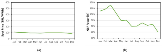
Figure 5.
NEWAVE historical simulation forecasts for 2019: (a) Spot price; and (b) GSF factor.
Figure 6 graphs the spot price and the GSF factor forecasts considering the CCEE deterministic scenario [26]. It is important to know that CCEE forecasts started in only 2016.
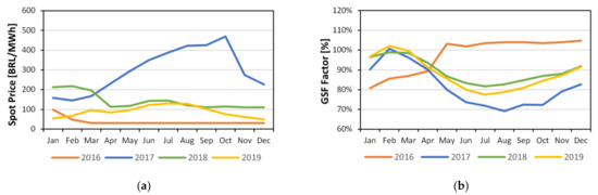
Figure 6.
CCEE forecasts for 2016 to 2019: (a) Spot price; and (b) GSF factor.
Figure 7 presents the FEC allocation that follows the ERM default criterion. It can be noted that the ERM default criterion represents a risk-averse strategic, with an allocation that varies only from 90% to 110%.
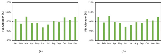
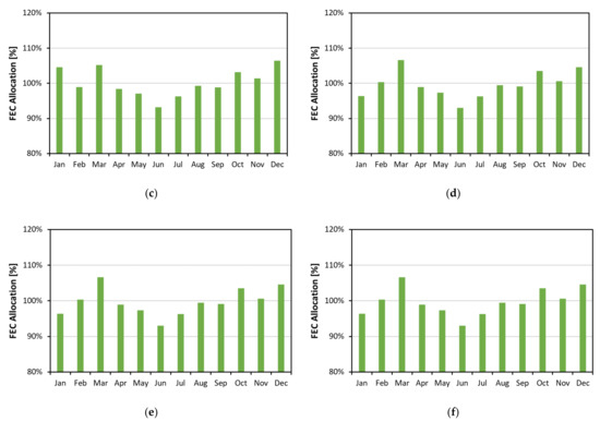
Figure 7.
ERM default allocation factor for the years: (a) 2014; (b) 2015; (c) 2016; (d) 2017; (e) 2018; and (f) 2019.
5.3. Results
Figure 8 presents the market intelligence tool results, considering the sum of all agents’ allocation decisions for the years 2014 to 2018.

Figure 8.
Results obtained for utility functions.
The results shown in Figure 8 indicate that, for the year 2014, the agents’ decision was based on the ERM default criterion with a 71% weight.
This pattern changed in 2015 with 88% weight on the NW spot price return. In 2016, it was not possible to infer a criterion with significant representativeness, as the Flat criterion was the major weight with 44% share. On the other hand, a higher participation of the GSF criterion can be noticed for 2017 and 2018, which considers CCEE GSF, accounting for 90% share in 2017, and NW GSF, having 100% share in 2018.
As explained in Section 5.1.2, Player 1′s (sum of all ERM agents) strategies of the game study are emulated by crossing the utility function results shown in Figure 8 and the FECMA factor for each criterion presented in Table 1 considering the variables’ forecasts for 2019. The FECMA factors for 2019 were calculated using the stochastic optimization model shown in Equations (1)–(6), and the values of 140% and 60% for and , respectively, were applied to these factors as premise. Table 2 shows the FECMA factors for 2019 utilized to project Player 1′s strategies, which are plotted in Figure 9.
Table 2.
FECMA factors for 2019 [%].
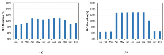
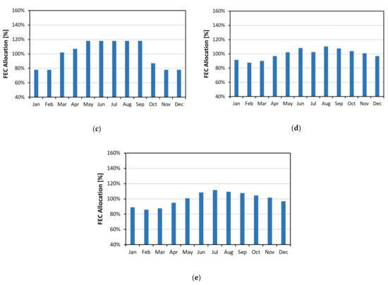
Figure 9.
Player 1’s strategies: (a) 2014; (b) 2015; (c) 2016; (d) 2017; and (e) 2018.
Figure 10 graphs Player 2′s (hydro generator with FEC equal to 1 MWavg) strategies for 2019 emulated by the stochastic optimization model and considering each criterion provided in Table 1. As a premise, the values of 160% and 40% for and , respectively, were applied. Furthermore, as explained in Section 5.1.2, to simplify the presentation of results, strategies with similar patterns were clustered in one profile, resulting in Player 2′s six strategies.
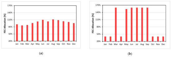
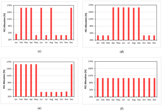
Figure 10.
Player 2’s strategies: (a) CCEE GSF; (b) CCEE spot price; (c) NW spot price return; (d) NW spot price CVaR; (e) NW spot price × GSF return; and (f) Flat.
Table 3 presents the payoff matrix obtained by applying the strategies shown in Figure 9 and Figure 10, where columns R.1 and R.2 represent the results of Player 1 and Player 2, respectively. From the matrix results, it can be noticed that, independently of Player 2′s strategy, Player 1 obtained a better payoff when opting for the same FEC decision allocation of 2017, eliminating all the other Player 1′s strategies by the iterated dominance method. Therefore, from Player 2′s perspective, the reduced matrix shows a better payoff associated with the NW spot price × GSF return strategy, resulting in the profile of strategies (2017, NW spot price × GSF return) as the Nash equilibrium of the game.
Table 3.
Payoff matrix [millions of BRL] (the proposed methodology was applied by Leonel [27], where similar results were found).
6. Discussion
This study presents a methodology of market intelligence and game theory tools considering the representativeness of stochastic behavior of some variables by applying a stochastic optimization model with an associated CVaR metric. The methodology also provides a more important aid, as compared to previous studies, to anticipate market behavior, providing strong support to rational decisions considering inherent decision-making process variables and constraints.
Using the FECMA decision methodology presented under the current Brazilian regulatory framework related to ERM, a behavioral change was noticed in the decision taken by the agents. Specifically, in 2015, the risk-neutral agents were inclined to maximize their expected return, indicating that their allocation decision was based on spot price forecasts, and in turn, the 2017 and 2018 results show the risk-averse agents defining their allocation decision in order to hedge themselves against the low hydro generation perspective. This behavioral change can be explained by the GSF factor’s decline in recent years, which motivates agents to apply an FECMA decision to hedge against spot market settlement in moments with a low GSF factor.
The application of the game theory model shows that the decision of a player with significant representativeness in the system in terms of FEC directly impacts the results of other players who have lower representativeness. Moreover, it was observed that when facing a decision-making process in a competitive environment, and if the other players’ strategies are unknown, it is better to decide on a strategy that culminates in greater payoff results, independent of other players’ strategies, even when this strategy is not the global optimal strategy.
The game theory results show that for the expected return payoff matrix, the Nash equilibrium corresponds to the profile of strategies in which the sum of ERM players apply 90% of the decision in the GSF factor forecast from the CCEE scenario (strategy 2017) and the unitary agent chooses the strategy resulting from the multiplication between the GSF and spot price forecast from NEWAVE scenarios considering one risk-neutral agent.
Some study limitations are related to the inability to analyze each ERM player as an individual. Future studies could examine in detail some ERM agents considered as big players, and for simplification, their results weighted by their FEC could be combined into a strategy that represents the total market decision. Other possible improvements are associated with agents’ portfolio contracts, where candidate contracts and flexibility causes can also be considered in the decision-making process.
This study pays particular attention to the payoff results from the expected return perspective. Future studies could evaluate the payoff from the risk perspective or use the convex function between risk and return weighted by the agent’s risk aversion profile. Additional future work may include forward contract customizations and the examination of the COVID-19 pandemic’s impact on the ERM process.
There has been a significant focus on ERM regulation in the past years because a constantly low GSF (less than 100%) causes players to question the operation dispatch. One of the recent regulation changes aimed to restrict the allocation limits for 2022 to a range based on the average of the last five years. The methodology and tools presented remain valid even with these changes but only within a restricted result subset.
7. Conclusions
In a very competitive environment such as the electricity wholesale market, the anticipation of other players’ strategies represents an important aid to support a decision-making process by decreasing the uncertainties regarding incomes and costs. Therefore, this article proposes a computational model based on stochastic optimization, combining market intelligence and game theory tools to emulate the market behavior and find the Nash equilibrium between the strategies forecasted for the market and the agent’s strategies.
The proposed methodology was applied to the FECMA decision process under the current Brazilian regulatory framework related to ERM, where the results show a distinct agents’ behavior to face the market price uncertainty, from neutral-risk agents seeking to maximize their results and focusing their decisions on spot price forecasts to risk-averse players trying to hedge against the hydrological risk.
Observing the Table 3 results, it can be noted that the proposed Player 2′s strategy (NW spot price × GSF return) has a lower expected return equal to BRL 0.178 million (when Player 1 chooses the 2014 strategy), which is 889% higher than its worst payoff (BRL 0.018 million when Player 2 adopts the NW spot price CVaR and Player 1 uses the 2015 strategy). In addition, the NW spot price × GSF return strategy presented greater results for Player 2 even when the Player 1 applied their dominant strategy (2017), resulting in a Player 2′s payoff being 5% higher than that in their lower scenario for this strategy.
Although this article focuses the study case on the ERM process under the Brazilian regulatory framework, the methodology can be easily readapted for any energy market situation where competition between the agents exists, representing an interesting tool to optimize a decision-making process into a competitive environment with uncertainties involved, where it is important to consider the associated risk and the other players’ strategies.
Supplementary Materials
The following are available online at https://www.mdpi.com/article/10.3390/en14196368/s1.
Author Contributions
Conceptualization: D.S.R., L.D.L. and M.H.B.; methodology: D.S.R., E.E.R., M.H.B. and L.D.L.; software: L.D.L. and M.H.B.; validation: D.S.R., E.E.R., M.H.B., L.D.L., and R.F.d.M.; formal analysis: L.D.L., M.H.B., and E.E.R.; investigation: L.D.L., M.H.B., E.E.R., and D.S.R.; resources: D.S.R. and R.F.d.M.; data curation: L.D.L. and M.H.B.; writing—original draft preparation: L.D.L. and M.H.B.; writing—review and editing: L.D.L., M.H.B., and D.S.R.; visualization: L.D.L. and M.H.B.; supervision: D.S.R.; project administration, D.S.R. All authors have read and agreed to the published version of the manuscript.
Funding
This research received financial support from the China Three Gorges Corporation, Brazil (CTG), through the Research and Development Project PD-07514-0117/2017 (ANEEL Code).
Data Availability Statement
The data presented in this study are available in supplementary material.
Conflicts of Interest
The authors declare no conflict of interest.
References
- Conejo, A.J.; Carrión, M.; Morales, J.M. Decision Making under Uncertainty in Electricity Markets; Springer: New York, NY, USA, 2010; Volume 1. [Google Scholar]
- Li, X.; Gao, L.; Wang, G.; Gao, F.; Wu, Q. Investing and pricing with supply uncertainty in electricity market: A general view combining wholesale and retail market. China Commun. 2015, 12, 20–34. [Google Scholar] [CrossRef]
- Pineda, S.; Conejo, A.J. Using electricity options to hedge against financial risks of power producers. J. Mod. Power Syst. Clean Energy 2013, 1, 101–109. [Google Scholar] [CrossRef] [Green Version]
- Fernandes, G.; Gomes, L.L.; Brandão, L.E.T. A risk-hedging tool for hydro power plants. Renew. Sustain. Energy Rev. 2018, 90, 370–378. [Google Scholar] [CrossRef]
- Valenzuela, P.; Lima, D.A.; Granville, S. A risk-constrained Energy Reallocation Mechanism for renewable sources with a Marginal Benefit approach. Electr. Power Syst. Res. 2018, 158, 297–305. [Google Scholar] [CrossRef]
- Vinel, A.; Mortaz, E. Optimal pooling of renewable energy sources with a risk-averse approach: Implications for US energy portfolio. Energy Policy 2019, 132, 928–939. [Google Scholar] [CrossRef]
- Birge, J.R.; Louveaux, F. Introduction to Stochastic Programming; Springer: New York, NY, USA, 1997. [Google Scholar]
- Rockfellar, R.T.; Uryasev, S.P. Optimization of Conditional Value-at-Risk. J. Risk 2000, 2, 21–41. [Google Scholar] [CrossRef] [Green Version]
- EPE. Decade Energy Plan 2029. Empresa de Pesquisa Energética. 2019. Available online: http://www.epe.gov.br (accessed on 1 October 2020).
- CEPEL. System Planning Models. Available online: http://www.cepel.br (accessed on 1 October 2020).
- Susteras, G.L.; Ramos, D.S.; Chaves, J.R.A.; Susteras, A.C.V.J. Attracting Wind Generators to the Wholesale Market by Mitigating Individual Exposure to Intermittent Outputs: An Adaptation of the Brazilian Experience with Hydro Generation. In Proceedings of the 8th International Conference on the European Energy Market (EEM), Zagreb, Croácia, 25–27 May 2011. [Google Scholar]
- Brasil. Lei nº 9648. 1998. Available online: http://www.planalto.gov.br/ccivil_03/Leis/l9648cons.htm (accessed on 1 October 2020). (In Portuguese)
- Machado, B.G.F.; Bhagwat, P.C. The impact of the generation mix on the current regulatory framework for hydropower remuneration in Brazil. Energy Policy 2019, 137, 111129. [Google Scholar] [CrossRef]
- CCEE. Market Information. Câmara de Comercialização de Energia. Available online: http://www.ccee.org.br (accessed on 2 October 2020).
- Dusse, A.C.S.; Lisboa, A.C.; Rodrigues, A.C.C.; Santos, F.F.G.; Saldanha, R.R. Equilíbrio de Nash e competição de Stackelberg na sazonalização no mercado de energia brasileiro. In Proceedings of the Simpósio de Engenharia de Produção (XXII SIMPEP), Bauru, SP, Brazil, 9–11 November 2015. (In Portuguese). [Google Scholar]
- Leonel, L.D.; Balan, M.H.; Camargo, L.A.S.; Rego, E.E.; Ramos, D.S.; Lima, R.M.F. Game Theory Application in Hydropower’s Firm Energy Monthly Allocation Process. IEEE Lat. Am. Trans. 2019, 17, 85–92. (In Portuguese) [Google Scholar] [CrossRef]
- Sokei, C.T. Model to Alocate the Assured Energy of Hydro Power Plants Using Genetic Algorithms. Ph.D. Dissertation, University of São Paulo, São Paulo/SP, Brazil, 2008. (In Portuguese). [Google Scholar]
- Santos, F.G.; Lisboa, A.C.; Vieira, D.A.G.; Saldanha, R.R.; Lobato, M.V. Formação de um perfil de sazonalização baseada em otimização multiobjectivo. In Proceedings of the Simpósio de Engenharia de Produção (XIX SIMPEP), Bauru, SP, Brazil, 5–7 November 2012. (In Portuguese). [Google Scholar]
- Greve, T.; Teng, F.; Pollitt, M.G.; Strbac, G. A system operator’s utility function for the frequency response market. Appl. Energy 2018, 231, 562–569. [Google Scholar] [CrossRef] [Green Version]
- Niromandfam, A.; Yazdankhah, A.S.; Kazemzadeh, R. Modeling demand response based on utility function considering wind profit maximization in the day-ahead market. J. Clean. Prod. 2019, 251, 119317. [Google Scholar] [CrossRef]
- Niromandfam, A.; Yazdankhah, A.S.; Kazemzadeh, R. Designing risk hedging mechanism based on the utility function to help customers manage electricity price risks. Electr. Power Syst. Res. 2020, 185, 106365. [Google Scholar] [CrossRef]
- Camargo, L.A.S.; Leonel, L.D.; Ramos, D.S.; Stucchi, A.G.D. A Risk Averse Stochastic Optimization Model for Wind Power Plants Portfolio Selection. In Proceedings of the 2020 International Conference on Smart Energy Systems and Technologies (SEST), Istanbul, Turkey, 7–9 September 2020; pp. 1–6. [Google Scholar] [CrossRef]
- Shapiro, A.; Tekaya, W.; da Costa, J.P.; Soares, M.P. Risk neutral and risk averse Stochastic Dual Dynamic Programming method. Eur. J. Oper. Res. 2013, 224, 375–391. [Google Scholar] [CrossRef]
- Fudemberg, D.; Tirole, J. Game Theory, 5nd ed.; MIT Press: Cambridge, MA, USA, 1996. [Google Scholar]
- CCEE/ONS. NEWAVE Outputs. Câmara de Comercialização de Energia / Operador Nacional do Sistema Elétrico. Available online: https://www.ccee.org.br (accessed on 5 October 2020).
- CCEE. InfoPLD Fev 2020. Câmara de Comercialização de Energia. 2020. Available online: http://www.ccee.org.br (accessed on 5 October 2020).
- Leonel, L.D. Game Theory and Market. Intelligence Applied to Hydroelectric Energy Allocation Strategies Aiming to Maximize Results and Control the Financial Risk in the Energy Reallocation Mechanism—ERM. Ph.D. Dissertation, Polytechnique School University of São Paulo, São Paulo, Brazil, 2020. (In Portuguese). [Google Scholar]
Publisher’s Note: MDPI stays neutral with regard to jurisdictional claims in published maps and institutional affiliations. |
© 2021 by the authors. Licensee MDPI, Basel, Switzerland. This article is an open access article distributed under the terms and conditions of the Creative Commons Attribution (CC BY) license (https://creativecommons.org/licenses/by/4.0/).