Article

Model-Free Power Control for Low-Voltage AC Dispatchable Microgrids with Multiple Points of Connection †

1
Instituto de Ciências Tecnológicas (ICT), Campus Itabira, Universidade Federal de Itajubá (UNIFEI), Itabira 35903-087, Brazil
2
Graduate Program in Electrical Engineering, Federal University of Minas Gerais (UFMG), Belo Horizonte 31270-901, Brazil
3
Campus of Rosana, São Paulo State University (UNESP), Rosana 19273-000, Brazil
4
Campus of Sorocaba, São Paulo State University (UNESP), Sorocaba 18087-180, Brazil
*
Author to whom correspondence should be addressed.
This work has financial support from Universidade Federal de Itajubá.
Energies 2021, 14(19), 6390; https://doi.org/10.3390/en14196390
Submission received: 13 August 2021 / Revised: 21 September 2021 / Accepted: 28 September 2021 / Published: 6 October 2021
(This article belongs to the Section A1: Smart Grids and Microgrids)

Abstract

:
This paper proposes a modified version of the power-based control (MPBC) applied to microgrids (µGs) with multiple points of connection (i.e., utility grid itself or any other neighboring µG). Using the MPBC, single-phase distributed energy resources (DERs) arbitrarily connected between the phases share the amounts of balanced power, while the unbalanced and homopolar power are steered only to the line-to-neutral inverters. The control technique is based on a three-level hierarchical control using narrow bandwidth, low data rate communication that properly coordinates the DERs connected to three-phase four-wire µGs. The MPBC allows the DERs to steer power flow at any of the multiple points of common coupling of a multi-PCC dispatchable µG. The modified control proposed herein is evaluated through simulation results using MATLAB/SIMULINK considering a real urban distribution grid with typical operational elements and conditions. When compared to the original power-based control (PBC), results show that a meshed µG may reach power benchmarks with accommodation time 80% lower when applying MPBC. Moreover, it may also lead to significant power loss reduction (about of 5%) in some studied cases.

1. Introduction

The microgrid (µG) model appears as a versatile structure to allow the interconnection of several distributed energy resources (DERs), loads and energy storage systems (ESSs) into a flexible grid topology [1]. Several references demonstrate that the µG model can increase grid efficiency, reliability and improve system stability [2,3]. Furthermore, if a µG is dispatchable in terms of power, it can contribute to increase the hosting capacity of a distribution system [4]. However, energy management and coordination of µGs become a challenge, since several uncertainties are involved in this assessment (e.g., intermittency in electricity sources, such as wind speed variation and solar shadowing, as well as variable load demand). If µG coordinated control is not well managed the ac bus may suffer from power quality (PQ) issues, such as voltage deviation, frequency variation, protection mistriggering etc., which can drive the system to instability [5,6]. In addition, a single µG has shortcomings to ensure resilience against disturbances at a certain point in the distribution grid [7].

1.1. Motivation

Considering those challenges, several studies have investigated the interaction between neighboring µGs, pursuing enhanced grid structures, system reliability and stability, while maximizing the use of DERs in µG clusters (µGCs) [8]. Some utility companies are already starting to adopt projects with µGCs, such as the Commonwealth Edison, which is developing a µGC using the Bronzeville µG and the campus µG at the Illinois Institute of Technology in Chicago [9]. µG cluster is defined as the interconnection of two or more µGs capable of connecting to the utility grid and exchanging power among them through their points of common coupling (PCCs) [6,10]. µGCs can also offer various ancillary services, including power flow control, energy trading, sharing of energy storage systems, corrective maintenance, frequency and voltage regulation in a larger geographic area of the electrical system, which allows for better system operation under contingency conditions [11]. However, if each µG in the cluster has its own goals and restrictions, there are new challenges for energy management systems (EMS) to ensure stable operation in terms of protection coordination, power flow control, voltage and frequency regulation, as well as protection of data shared between µGs [12].

1.2. Literature Review

In such context, the authors of [13] analyze the dynamic behavior of µGCs composed of radial µGs and DERs with photovoltaic energy sources controlled by the droop technique. Different approaches of centralized and decentralized control, and even the combination of both are being applied to overcome the challenges of coordinated control of DERs in µGCs [14]. In this regard, in [8] a flexible strategy of division and unification with dispersed communication is used to increase the resilience of a µGC formed by three µGs. In [15] a decentralized energy dispatch model is proposed for the coordinated operation of several µGs and a distribution system. The problem is based on a two-level decentralized stochastic optimization algorithm, with µGs at the lower level and the main grid at the upper level. However, the internal structure of the µGs and the control technique of the DERs are neglected, as well as the power flow between the µGs. The authors of [16] propose an optimization algorithm combined with a communication system to manage µGCs. This approach aims at minimizing operating costs and meeting the internal power balance in µGs. However, the internal structure of µGs and the DERs control technique are not addressed.
The authors of [17] propose a central EMS that uses a two-tiered hierarchical control scheme for the utility and several electrically coupled µGs. In that paper [17], the primary level controllers are based on droop technique and the µGs assume radial topology. The authors of [18] present a hierarchical and distributed cooperative control architecture for islanded µGCs. The proposed two-layer four-level control architecture can protect proprietary information and enable the plug-and-play capability of each µG. However, the technique is analyzed considering only radial µGs. In [19], an EMS is formulated as a stochastic linear programming problem. The hierarchical control structure is responsible for the frequency regulation on the islanded µGC. The connection between the three µGs is performed by three back-to-back converters forming a triangle with the µGs in the vertices. The controllers in the primary level are based on the droop technique and the µGs assume radial topology. However, the system has the disadvantages of high financial cost and reduced reliability due to the high number of power converters. The authors in [20] present a two-layer distributed secondary control strategy that allows voltage and frequency regulation and accurate power sharing in each µG of an islanded µGC with series topology. However, the energy exchange among the μGs is not analyzed and only three-phase DERs are used.
In [21] a two-level algorithm to coordinate energy trade among µGCs and distribution system operator (DSO) is proposed. The strategy consists in reconfiguring the distribution system to optimize energy costs. However, this approach is model-based, requiring distribution grid information such as line connections and impedance values and current ratings of feeders. In [21], the primary level controllers are based on droop technique and the µGs assume radial topology. In [22], a method is proposed to restore a distribution system in several microgrids, taking into account the demand-side three-phase management. However, this technique is model-based and requires several parameters of the electrical system for its implementation. The authors of [23] introduce an optimal control approach for poly-phase smart grids of whatever structure, topology, variety of power sources, loads, storage units, and multiple points of connection to the utility grid. However, it is a model-based approach and it has the same limitations and drawbacks as highlighted previously for [21,22].
The PBC control strategy was originally proposed to proportionally coordinate the power sharing between the DERs in single-phase µGs. It has evolved to increase its benefits and applicability, as summarized in Table 1 underlining the main changes that the PBC has undergone in recent years. The strategy proposed herein inherits the main characteristics of the PBC such as: (i) minimum requirements in terms of information and communication technology (ICT); (ii) it does not require prior knowledge of power grid parameters (i.e., it is a model-free approach); (iii) it has accurate regulation of active/reactive power to meet DSO hosting capacity limits (i.e., PQ requirements); (iv) support to plug-and-play integration of new DERs); and (v) it is implemented in the secondary control level of the µG. Thus, previously published PBC papers sought to increase the range of PBC application (i.e., types of DERs, µGs topologies, benefits, etc.). However, the decomposition of active and reactive power in balanced, unbalanced, and homopolar components, which may improve the power sharing capability among DERs with distinct types of connection in the µG (i.e., line-to-line and line-to-neutral), has not been considered in the previous PBC definitions.

1.3. Contributions and Paper Organization

Seeking the coordinated operation of single-phase DERs, arbitrarily connected between phases and coexisting in a µG, this paper proposes the following innovative contributions:
An improved version of the PBC (i.e., MPBC) that treats the arbitrary inverter connections (i.e., line-to-line and line-to-neutral) in a proper and individual manner to increase the degree of freedom of the control strategy. Thus, the objective is to make each DER process only the power terms that fit into its type of connection (i.e., line-to-line and line-to-neutral). To do so, different scalar coefficients are defined for single-phase line-to-line and line-to-neutral DERs, which doubles the degree of freedom of the PBC algorithm in relation to its previous versions. Hence, accurate power sharing among the DERs and unbalance current compensation are achieved if line-to-line DERs and line-to-neutral DERs share balanced power components, while unbalanced and homopolar power components are steered to line-to-neutral DERs. Also, MPBC results in faster dynamic response and lower grid power losses than the conventional PBC and it is self-adjusted to different grid topologies.
In addition, a power flow control strategy is presented for meshed µGs with multiple PCCs. This scenario has not yet been explored in the literature with the use of PBC, and it is analyzed in this paper as a case study of the MPBC application to control one PCC of the meshed µG at a time, according to the references defined by the DSO.
The paper is organized as follows: Section 2 describes the µG topology, elements, and the hierarchical control. Section 3 presents the formulation of MPBC. Section 4 shows the simulation results comparing PBC with MPBC in a real urban distribution grid, and the results of MPBC applied to grid power control of a multiple PCC µG. Finally, Section 5 presents some conclusions.

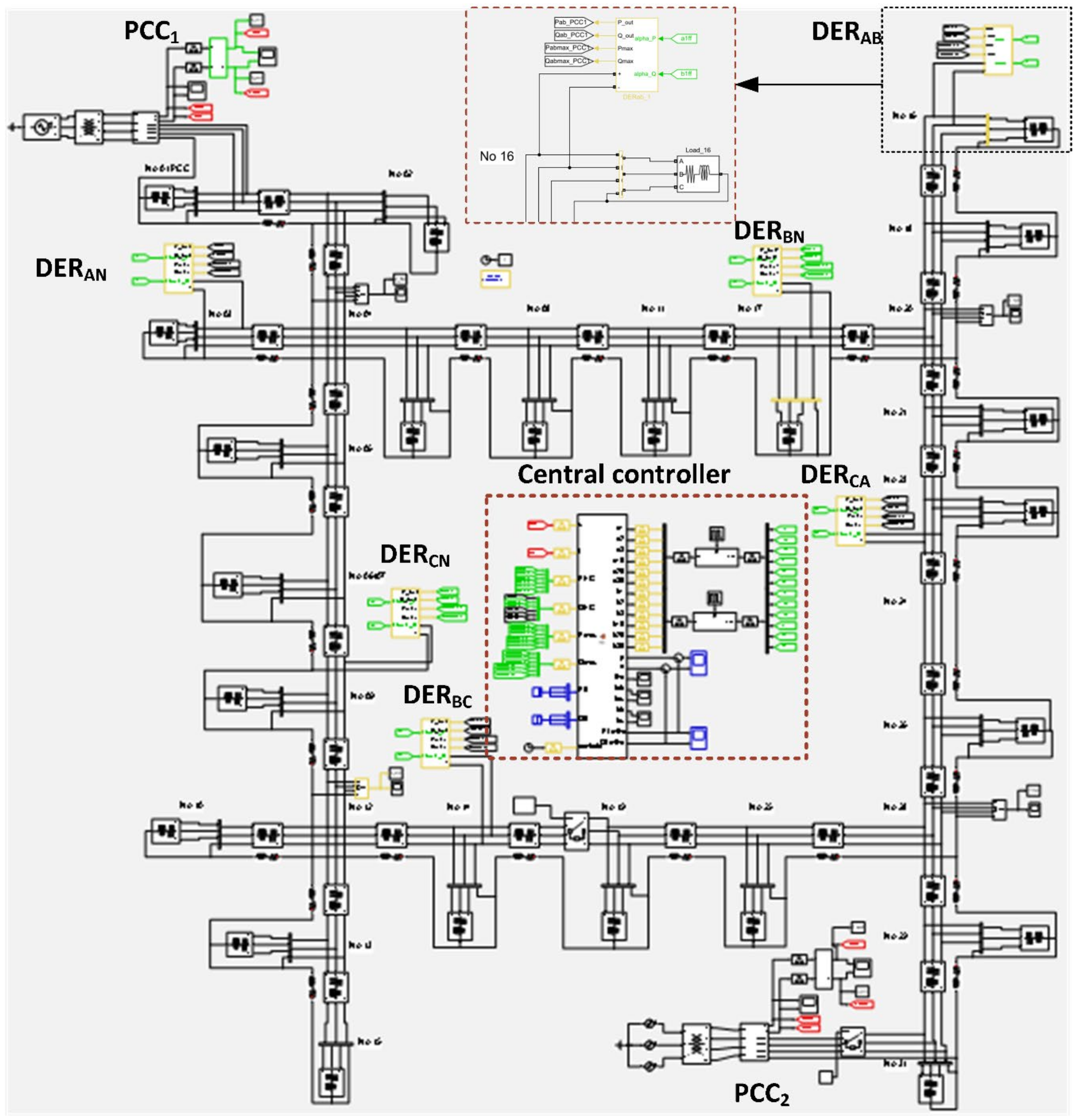
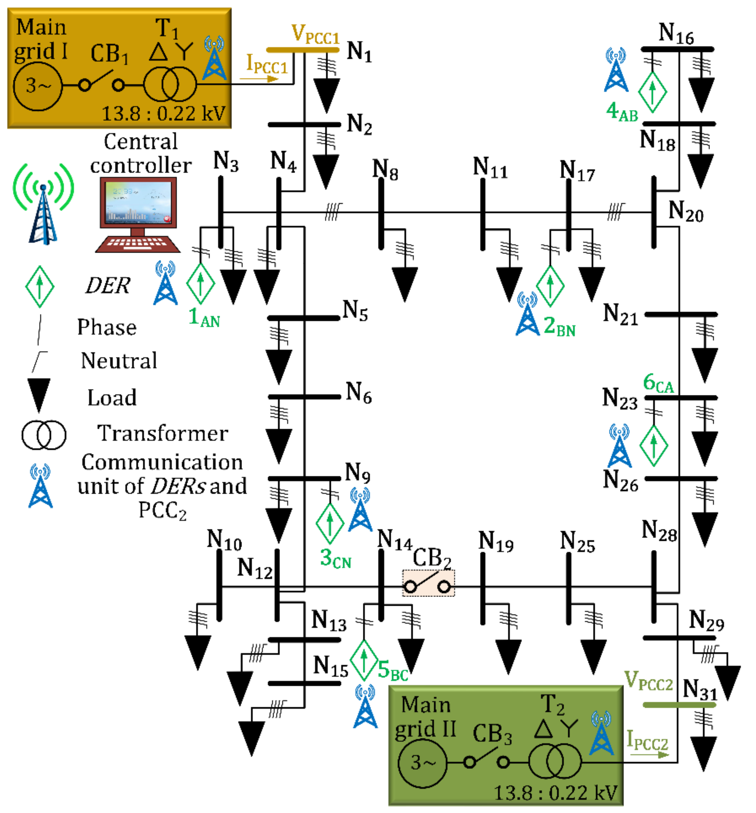
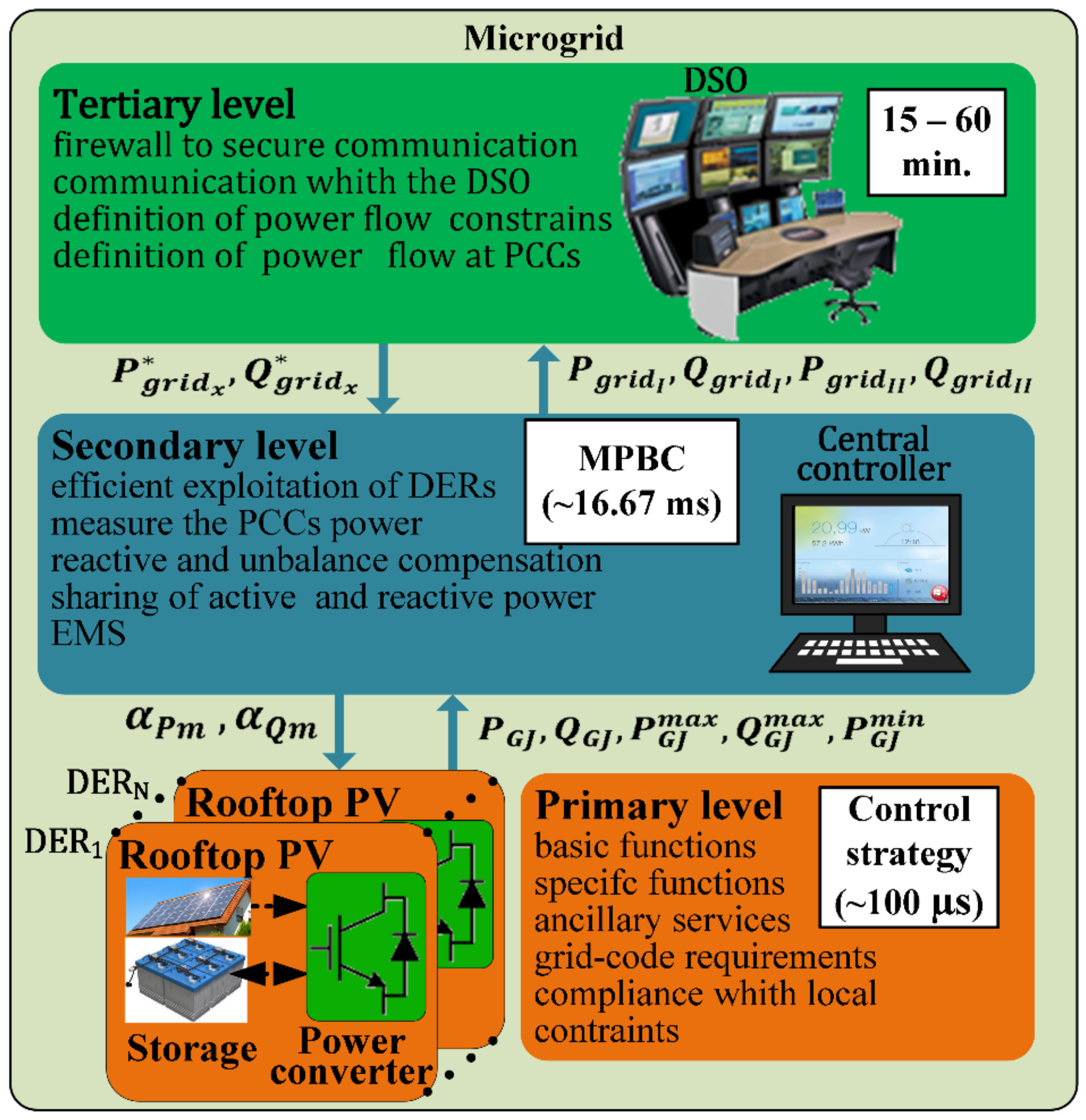
2. Structure, Topology and Control Approach of the Microgrid Testbench

The µG may operate assuming distinct topologies, such as radial, meshed, or mixed. From these three topologies, the last two have the following advantages in comparison to radial µGs: (i) lower-level values of voltage fluctuation; and (ii) more reliability (since the load demand is supplied by one or more PCCs). Such features are appealing under weak grid and during power outages. On the other hand, meshed and mixed grids have a more complex structure than radial grids, thus the EMS becomes a challenging task [6]. Thus, considering that most of the papers in literature have addressed radial µGs [8,10,17,18,19], this paper contributes with the analysis of dispatchable µGs assuming meshed topology with multiple points of connection.
To analyze the MPBC algorithm proposed herein, a three-phase four-wire urban distribution grid is used as a case study testbench, as shown in Figure 1. It is supplied from two different feeders at two distinct PCCs, N1 and N31 where “N” represents the node. Also, two identical transformers with a delta-wye configuration of 13.8 kV at the primary side and 220 V (line-to-line) at the secondary side are used. The grid comprises heterogeneous line impedances between the nodes, and the unbalanced loads are unevenly distributed among the phases. In addition, six dispersed single-phase DERs are arbitrarily connected between the system phases (phase a: DERN3; phase b: DERN17; phase c: DERN9, ab phases: DERN16; phases bc: DERN14 and ca phases: DERN23).
The islanded operation and the smooth transition between the islanded and grid-connected modes should be performed by means of a three-phase grid interactive converter called a utility interface as discussed in [27]. Such a converter must operate as a grid-supporting converter during µG grid-connected mode, whereas it operates as grid-forming converter when the µG is islanded. However, these analyses are not addressed in this paper, and the utility interface is not included in Figure 1.
The distribution power system has three circuit breakers that allow the grid topology to be re-arranged from meshed to radial, and vice versa. Such flexibility increases the grid resilience and reliability since the µG can operate in both topologies and be supplied by PCC1, PCC2 or both, as shown in Table 2. The operating modes change in case of abnormal operation or by technical and/or economic interests of the µG itself or DSO.
The control organization of the system is based on a hierarchical architecture of a centralized controller, where the central controller (CC) is responsible for cooperatively conducting the operation of DERs through a narrow bandwidth, low data rate communication link. A recurring control process is implemented by collecting and processing information related to the average power from DERs, as well as the grid power flow through the two PCCs. After data processing, scalar coefficients are broadcasted by the CC to the DERs to define locally the power references for each DER. The µG control strategy requires a two-way communication infrastructure linking CC and DERs, which due to the characteristics of the PBC are easily implemented by interoperability standards such as IEC 61850 [28]. Commercial microgrid controllers, such as EcoStruxure from Schneider Electric [29] and GridNode from General Electric [30], could be used for such an application.
The hierarchical control architecture adopted is shown in Figure 2, and it is divided into three levels according to the updating frequency of the variables, dependence on communication and the imperative actions for proper operation of the µG. The primary level is the fastest one, running with processing frequencies of a few kHz, and being responsible for the local and autonomous control of DERs. This means that it is in charge of basic and specific functions to meet grid-code requirements, such as: voltage, current, frequency and synchronization control that are directly related to the stability of the power system, i.e., independent of communication [31]. As the primary level is well consolidated in the literature [32], it is not addressed herein.
The secondary level is fully implemented in the CC, on which the MPBC algorithm is executed using a bidirectional communication link to perform the exchange of data with the DERs. This level acts for the sharing of proportional power, based on the electrical quantities from the PCCs and DERs in the current control cycle. After collecting data by the CC and processing the MPBC, the new portion of power is sent to the DER as a power reference to the next control cycle. This control level operates within millisecond scale (i.e., around the line frequency) and aims at improving the system efficiency and the PQ of the µG. Therefore, the secondary level relies on communication; however, if communication is lost, the µG still operates assuming the functionality of the primary level.
The tertiary level is the slowest one (from a few minutes to hours) and it is updated a few times a day. It is based on a highly secure bidirectional communication link interconnecting the DSO to the µG / µGC. The tertiary level is committed to managing the interoperability between µG and DSO or between neighboring µGs, in terms of maximum and minimum restrictions of active/reactive power flow, based on the hosting capacity of the system.

3. Modified Power-Based Control (MPBC)

This section presents the model-free modified PBC algorithm (MPBC) capable of remotely regulating DERs coexisting in a µG of meshed topology and multiple PCCs. An innovative aspect of MPBC is that this formulation allows the distinction between line-to-line and line-to-neutral DERs, which provides a greater degree of freedom to the µG secondary level control. In such a scenario, accurate power sharing among DERs and unbalance current compensation are promptly achieved if line-to-line DERs and line-to-neutral DERs share balanced power, while unbalanced and homopolar power terms are steered to line-to-neutral DERs. This allows DERs with different connection features to operate with different scalar coefficients, which is not possible with the conventional PBC. Further details of the PBC formulation are shown in [25].
Finally, the greater degree of freedom of MPBC in comparison with PBC drives the system to: (i) reduced power losses; and (ii) faster dynamic response. In the following sections, terms with _ are vectors or matrices; and their elements are indexed with m or n for line-to-neutral quantities and mn for line-to-line quantities. Also, function d i a g ( ) stands for vector transformation to a square matrix filled with the vector elements in the diagonal and zeros otherwise. Figure 3 shows the flowchart with the sequence of execution of the proposed algorithm.

3.1. Power Quantities at the µG Points of Common Coupling (PCCs)

Considering the control cycle l and the next control cycle ( l 1 = l + 1 ,) whether P _ P C C x l , Q _ P C C x l , P _ P C C x l 1 , Q _ P C C x l 1 , are the vectors with active and reactive power exchanged with the main grid in the three µG phases. Terms with subscript   P C C   x   are provided by the grid at the PCC being controlled. The subscript X = 1 , 2   indicates which PCC is controlled, and (*) indicates the power references for the PCCX.
To steer the power references in the PCCs ( P _ P C C x l 1 , Q _ P C C x l 1 ), the CC broadcast power commands to the DERs according to their characteristics, such as the type of connection of each DER (line-to-neutral or line-to-line). In this way, the following power quantities are presented:
Homopolar power ( P _ P C C x h o and Q _ P C C x h o ): the power components of these vectors are calculated for each PCC phase considering only the homopolar components of the currents, which are extracted by using i h o = m = 1 3 i m / 3 .
An inherent characteristic of the homopolar power is that m = 1 3 P P C C x m h o = m = 1 3 Q P C C x m h o = 0 . Also, it is possible to calculate the vectors of non-homopolar power at the PCC phases as: P _ P C C x n h o = P _ P C C x P _ P C C x h o and Q _ P C C x n h o = Q _ P C C x Q _ P C C x h o .
Balanced power ( P _ P C C x b and Q _ P C C x b ): these vectors represent a three-phase balanced load-equivalent power consumption, and their elements are calculated for each phase in function of the rms values of the PCC line-to-neutral voltages as:
P P C C x m b = n = 1 3 P P C C x n n h o n = 1 3 V n 2 · V m 2 Q P C C x m b = n = 1 3 Q P C C x n n h o n = 1 3 V ^ n 2 · V ^ m 2
Moreover, the difference between balanced power and non-homopolar power results in unbalanced power quantities as:
P _ P C C x u = P _ P C C x n h o P _ P C C x b Q _ P C C x u = Q _ P C C x n h o Q _ P C C x b
Also, note that:
m = 1 3 P P C C x m b = m = 1 3 P P C C x m n h o ,   m = 1 3 Q P C C x m b = m = 1 3 Q P C C x m   n h o , m = 1 3 P P C C m u = m = 1 3 Q P C C m u = 0

3.2. Power Transformation Matrices

Considering the presence of line-to-line DERs in the µG, the line-to-line power quantities is converted to line-to-neutral equivalent quantities (and vice versa) by the matrices:
A _ = V 1 2 v 1 , v 2 0 V 1 2 v 3 , v 1 V 2 2 v 1 , v 2 V 2 2 v 2 , v 3 0 0 V 3 2 v 2 , v 3 V 3 2 v 3 , v 1
B _ = V ^ 1 2 v ^ 1 , v ^ 2 0 V ^ 1 2 v ^ 3 , v ^ 1 V ^ 2 2 v ^ 1 , v ^ 2 V ^ 2 2 v ^ 2 , v ^ 3 0 0 V ^ 3 2 v ^ 2 , v ^ 3 V ^ 3 2 v ^ 3 , v ^ 1
Matrices A _ and B _ are deduced from equations of delta-wye impedance transformation. The terms of matrices A _ and B _ correspond to line-to-neutral voltages v 1 ,   v 2 , v 3 and their respective homo-integrals ν ^ 1 , v ^ 2 , v ^ 3 and rms values V 1 ,   V 2 , V 3 , V ^ 1 ,   V ^ 2 , V ^ 3 , and ; indicates internal product operation.
Thus, in the following relationships, P _ l n and Q _ l n are vectors with line-to-neutral quantities; P _ l l and Q _ l l are vectors with line-to-neutral quantities; V _ l l and V ^ ¯ l l are vectors with square rms values of the line-to-line voltages and their homo-integrals:
P _ l n = A _ · d i a g V _ l l 1 · P _ l l P _ l l = d i a g V _ l l · A _ 1 · P _ l n
Q _ l n = B _ · d i a g V ^ ¯ l l 1 · Q _ l l Q _ l l = d i a g V ^ ¯ l l · B _ 1 · Q _ l n

3.3. Data Packet of the MPBC Distributed Energy Resources (DERs)

Considering a J number of DERs connected to the µG at the control cycle l , the data that the j t h DER exchange with the CC is:
Active and reactive power injected into the µG: P G j l ,   Q G j l ;
Maximum active P G j m a x l and reactive Q G j m a x l power it can inject into the µG: P G j m a x l varies according to the available energy resources of each DER at the cycle l , while Q G j m a x l depends on P G j m a x l and the nominal power of the DER;
Maximum active power that it can absorb from the µG: P G j m i n l .

3.4. MPBC Algorithm

Step 1: during the control cycle l , after receiving the data packet from the DERs, the CC calculates the vectors of total injected power and maximum power capacities by phase ( P _ G l n l , Q _ G l n l , P _ G l n m a x l , Q _ G l n m a x l ) and between phases ( P _ G l l l , Q _ G l l l , P _ G l l m a x l , Q _ G l l m a x l ). The elements of these vectors are computed by summing the power quantities of the DERs at phase m = 1 ,   2 ,   3 or between phases m n = 12 ,   23 ,   31 :
P G l n _ m l = j = 1 J P G j _ m l Q G l n _ m l = j = 1 J Q G j _ m l
P G l l _ m n l = j = 1 J P G j _ m n l Q G l l _ m n l = j = 1 J Q G j _ m n l
P G l n _ m m a x l = j = 1 J P G j _ m m a x l Q G l n _ m m a x l = j = 1 J Q G j _ m m a x l
P G l l _ m n m a x l = j = 1 J P G j _ m n m a x l Q G l l _ m n m a x l = j = 1 J Q G j _ m n m a x l
Step 2: The CC calculates the power reference for the DERs to the next control cycle l 1 = l + 1 considering the characteristics of each DER connected to the µG:
If there are only line-to-line connected DERs in the µG, their power references are calculated by:
P _ G l l l 1 = d i a g V _ l l · A _ 1 · P _ P C C x b l P _ P C C x l 1 + P _ G l l l
Q _ G l l l 1 = d i a g V ^ ¯ l l · B _ 1 · Q _ P C C x n h o l Q _ P C C x l 1 + Q _ G l l l
Equations (12) and (13) address balanced active power and reactive power to the line-to-line DERs and neglect the homopolar power, which cannot be injected by line-to-line connected DERs. In this case, the reactive power injected by the line-to-line DERs compensates unbalance power consumption caused by non-homopolar currents.
If there are only line-to-neutral connected DERs in the µG, no power decomposition is necessary since the line-to-neutral connection allows a complete phase-decoupled power injection. Thus, the power references are computed as:
P _ G l n l 1 = P _ P C C x l P _ P C C x l 1 + P _ G l n l
Q _ G l n l 1 = Q _ P C C x l Q _ P C C x l 1 + Q _ G l n l
If both line-to-line and line-to-neutral DERs are connected to the µG, these two types of DERs can share the PCC power demands. To do so, let P _ G l n m a x l and Q _ G l n m a x l be the maximum power capacities obtained from P _ G l l m a x l and Q _ G l l m a x l using (6) and (7). Then, the vectors of demand-sharing coefficients are defined as:
c _ P l = d i a g P _ G l n m a x l + P _ G l n m a x l 1 · P _ G l n m a x l
c _ Q l = d i a g Q _ G l n m a x l + Q _ G l n m a x l 1 · Q _ G l n m a x l
and the power shared are calculated as:
P _ l n s h l = d i a g c _ P l ·   P _ P C C x b l P _ P C C x l 1
Q _ l n s h l = d i a g c _ Q l · Q _ P C C x b l Q _ P C C x l 1
P _ l n s h l = I _ d i a g c _ P l ·   P _ P C C x b l P _ P C C x l 1
Q _ l n s h l = I _ d i a g c _ Q l · Q _ P C C x b l Q _ P C C x l 1
in which I _ is the identity matrix. Hence, the power references for the line-to-neutral DERs are:
P _ G l n l 1 = P _ l n s h l + P _ P C C x u l + P _ P C C x h o l + P _ G l n l
Q _ G l n l 1 = Q _ l n s h l + Q _ P C C x u l + Q _ P C C x h o l + Q _ G l n l
and for the line-to-line DERs:
P _ G l l l 1 = d i a g V _ l l · A _ 1 · P _ l n s h l + P _ G l l l
Q _ G l l l 1 = d i a g V ^ ¯ l l · B _ 1 · Q _ l n s h l + Q _ G l l l
In conclusion, the line-to-line DERs and line-to-neutral DERs share the balanced power quantities, while the unbalanced and homopolar power quantities are handled by the line-to-neutral DERs.
Step 3: The CC calculates the power commands for each type of DER in function of the power references and the maximum capacities:
For the line-to-line connected DERs:
α _ l l P = d i a g P _ G l l m a x l 1 · P _ G l l l 1
α _ l l Q = d i a g Q _ G l l m a x l 1 · Q _ G l l l 1
For the line-to-neutral DERs:
α _ l n P = d i a g P _ G l n m a x l 1 · P _ G l n l 1
α _ l n Q = d i a g Q _ G l n m a x l 1 · Q _ G l n l 1
In both cases, if any element of the vectors is greater than unity, it is limited in 1.

3.5. Power References in Each DER

On the local controller of each DER, the power references for the control cycle l 1 = l + 1 are calculated in function of the power commands sent by the CC and the DERs’ power capacities, as expressed in the following:
On the j t h DER connected between phases m and n :
P G j l 1 = α l l _ m n P · P G j m a x l Q G j l 1 = α l l _ m n Q · Q G j m a x l
On the j t h DER connected between phase m and the neutral conductor:
P G j l 1 = α l n _ m P · P G j m a x l Q G j l 1 = α l n _ m Q · Q G j m a x l

4. Simulation Results

Several computational simulations were carried in order to evaluate the proposed MPBC strategy in comparison to the conventional PBC. The low-voltage (LV) µG testbench, previously described in Section 2 and shown in Figure 1, is simulated in MATLAB/SIMULINK, on which the control algorithms and the hierarchical control are processed as well. As shown in Figure 2, the MPBC sited in the secondary control level is carried out at each cycle of the fundamental grid voltage (i.e., 16.67 ms). The CC receives data from the DERs at the same time base and updates the scalar coefficients of the DERs every three cycles (i.e., 50 ms). The µG line impedance values, nominal load capacities and parameters of delta-wye transformers are described in [33]. The parameters of the DERs are shown in Table 3. Figure A1 in Appendix A shows the simulation platform developed in MATLAB/SIMULINK.
The analyses are undertaken using two scenarios out of the six presented in Table 2. Thus, different operational conditions are considered to: (i) evaluate the response time of the MPBC to reach the power references in comparison to PBC; (ii) show the µG losses reduction when applying MPBC; (iii) evaluate the proposed method for accurately sharing power among DERs; and (iv) precisely regulate the grid power flow through multiple PCCs in an urban LV µG.

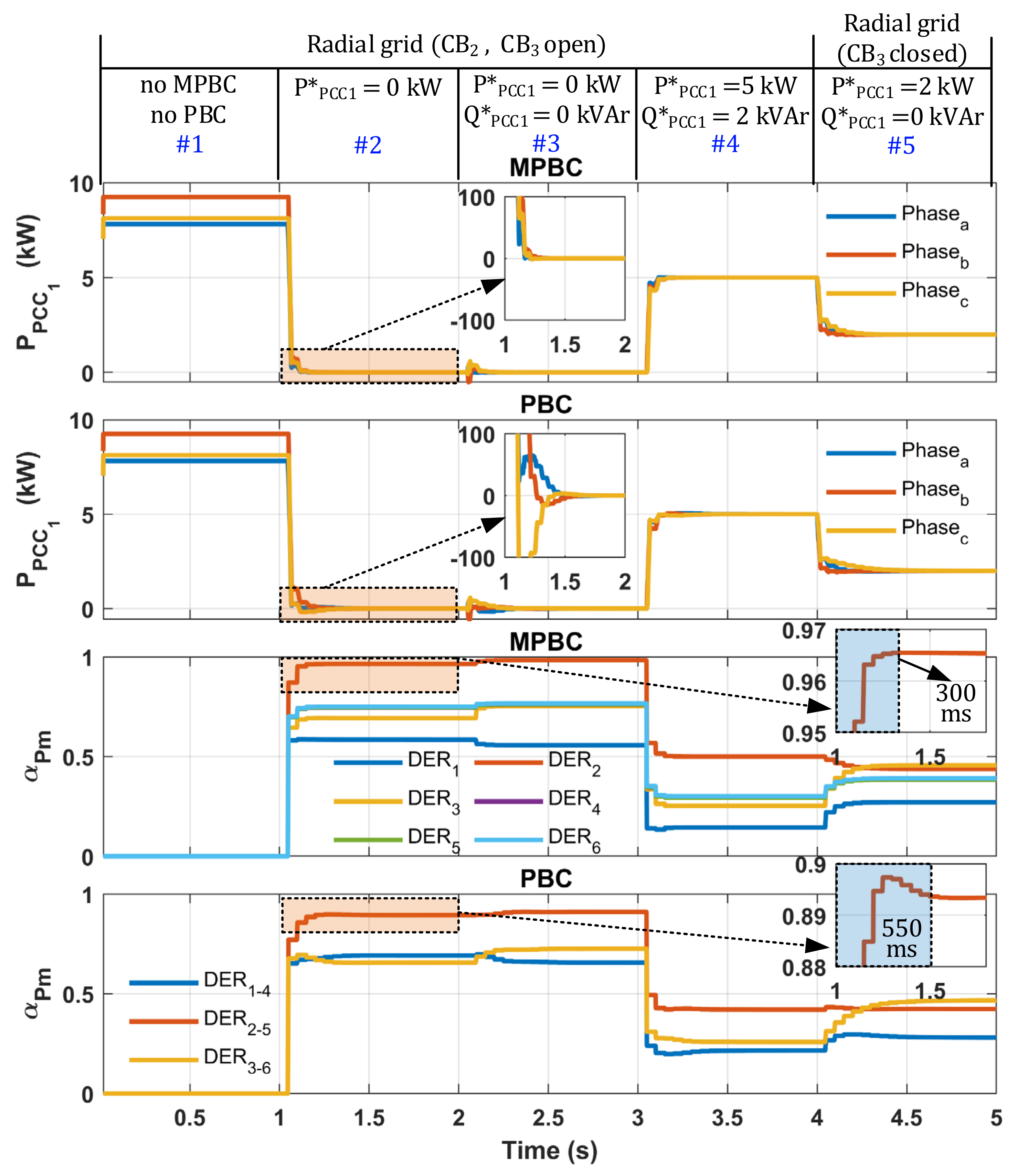
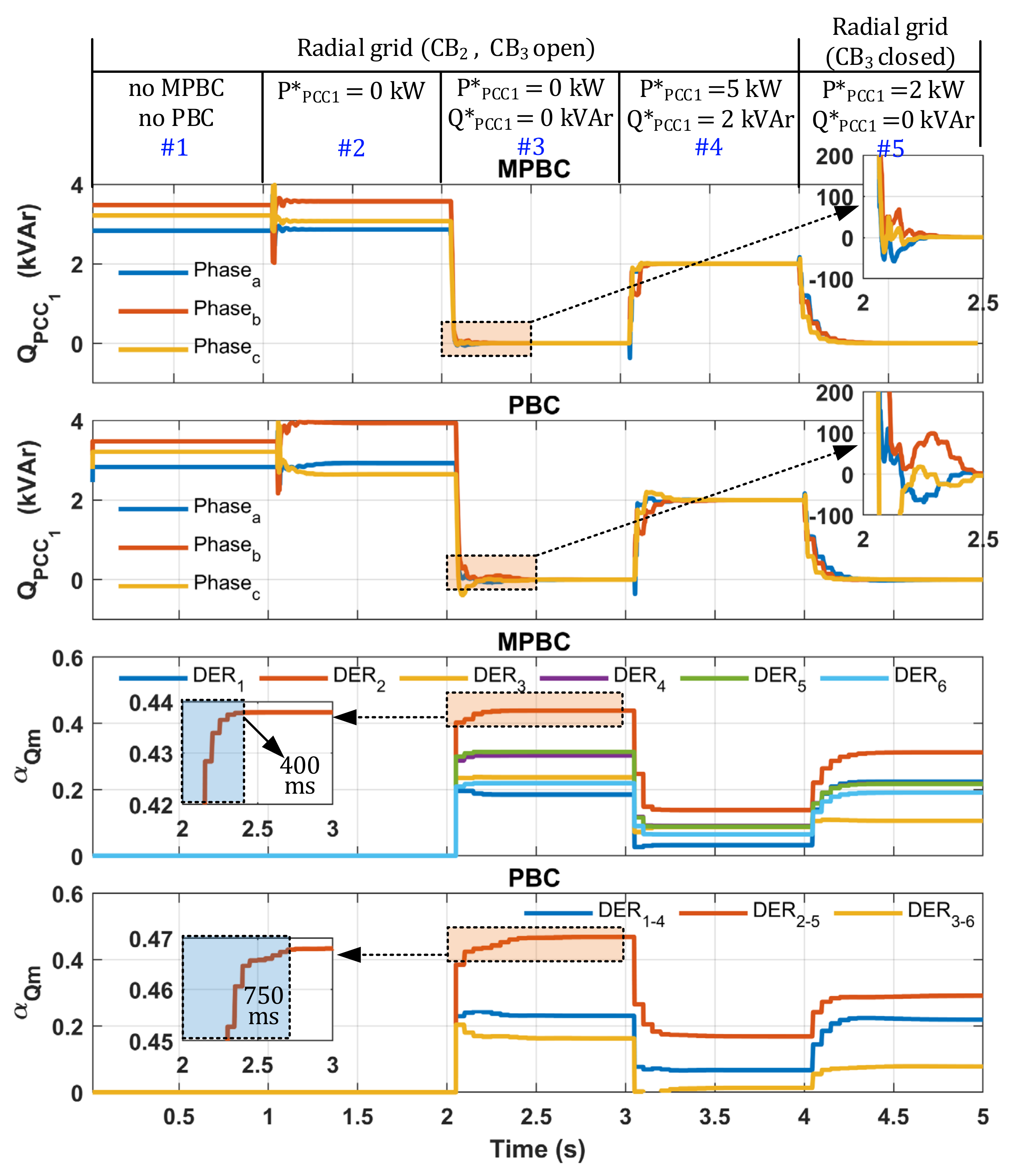
4.1. Comparison between MPBC and PBC

The MPBC and PBC are evaluated against different operating conditions to assess the main differences of the two approaches. Figure 4 and Figure 5 comprise the five operating conditions used in this case study, such that:
Interval #1, the DERs are disabled, and the load demand is fully supplied by the mains itself through PCC1.
At instant 1 s (interval #2), the algorithm is enabled and starts to control only active power through the PCC1 considering P _ P C C 1 l 1 = 0 .
At instant 2 s (interval #3), active and reactive power references in PCC1 are: P _ P C C 1 l 1 = 0 , Q _ P C C 1 l 1 = 0 .
At instant 3 s (interval #4), active and reactive power references in PCC1 are: P _ P C C 1 l 1 = 5   kW , Q _ P C C 1 l 1 = 2   kVAr .
Finally, at instant 4 s (interval #5), CB3 is closed, and the µG starts to operate with two PCCs. The power references in PCC1 are: P _ P C C 1 l 1 = 2   kW , Q _ P C C 1 l 1 = 0   kVAr .
During all intervals the µG assumes the radial topology, but between intervals #1 and #4 it is supplied only by PCC1. Then, during interval #5 the µG is supplied by PCC1 and PCC2.
As a numerical example to clarify the application of MPBC algorithm, Table 4 presents the values of all MPBC quantities calculated at four instants of the µG simulation in this case study. The corresponding equations from Section 3 are also indicated.
Figure 4 shows active power in the PCC1 and scalar coefficients α P m for both algorithms. It is observed that the MPBC requires a shorter accommodation time in comparison with PBC to accomplish the active power references at the PCC. To quantify the accommodation time during power reference changes for both control algorithms, the coefficients α P m in Figure 4 are used. MPBC needs 300 ms to achieve steady-state value corresponding to the portion of active power that DER2 must provide. Whereas PBC requires 550 ms, that corresponds to 83.3% of increase in time.
Figure 5 shows the reactive power through PCC1 for MPBC and PBC. It can be seen in Figure 5 that the reactive coefficients α Q m require longer accommodation time compared to the active power in Figure 4. Therefore, that MPBC needs 400 ms to accommodate the reactive power reference, while PBC requires 750 ms, which corresponds to an increase of 87.5%. In interval #4, the active and reactive power references at PCC1 are changed simultaneously. From Figure 4 and Figure 5, it is notable that both algorithms can reach the reference values; however, the MPBC has shorter accommodation time.
Finally, the analysis of losses in µG for the two algorithms in view of the different operating conditions is shown in Figure 6, considering that the power losses are quantified using (32).
P l o s s k = n = 1 N R n · I n 2
such that Rn is the resistance of the n-th grid power line and In is the current flowing through Rn.
During interval #1, when the DERs are not exchanging power, the loss is identical for both. However, from the interval #2, when the DERs share their power proportionally, the MPBC shows lower losses than the PBC in all the scenarios evaluated. The maximum reduction obtained with MPBC occurs at interval #4 with 4.85% of reduction. The minimum value occurs at interval #5 when µG is fed by two PCCs, reaching the level of 2.56%.

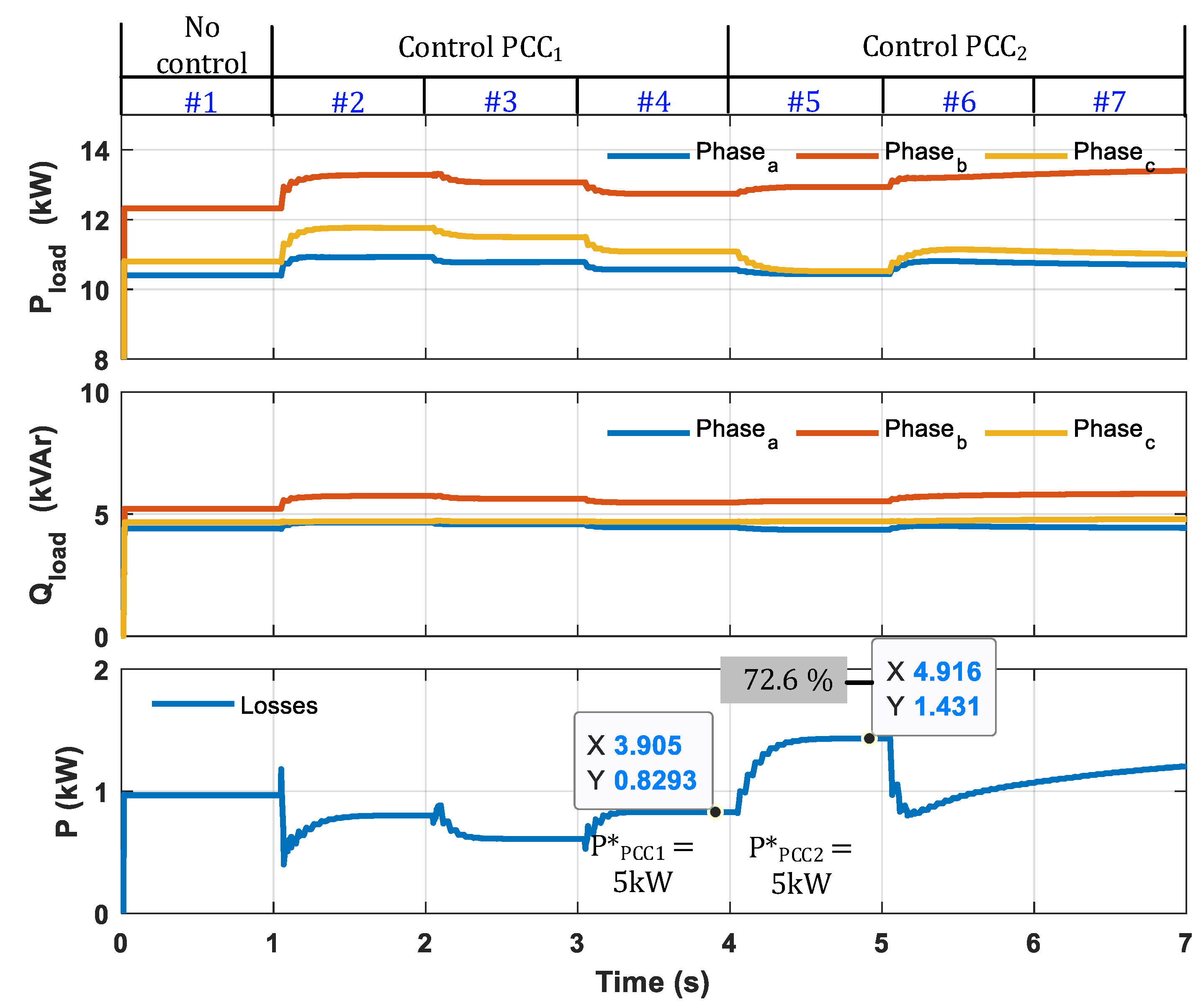
4.2. MPBC Applied to Meshed µG with Multiple PCCs

In this section, the proposed MPBC is applied to the µG testbench configured as meshed multi-PCC µG. The CC receives from DSO the power references for both PCCs. In this scenario, the DERs are driven to supply the demand in a specific PCC according to technical, economic, external and internal restrictions of µG. The operating conditions used during the test are:
Interval #1: DERs are disabled, and the load demand is fully supplied by the mains itself through PCC1 and PCC2.
At instant 1 s (interval #2), the algorithm is enabled with power control on PCC1 with the following references: P _ P C C 1 l 1 = 0   kW , Q _ P C C 1 l 1 = 0 .
At instant 2 s (interval #3), power references to PCC1 are defined as: P _ P C C 1 l 1 = 2   kW , Q _ P C C 1 l 1 = 0 .
At instant 3 s (interval #4), power references to PCC1 are defined as: P _ P C C 1 l 1 = 5   kW , Q _ P C C 1 l 1 = 0 .
At instant 4 s (interval #5), the DSO changes the power references for PCC2, thus P _ P C C 2 l 1 = 5   kW , Q _ P C C 2 l 1 = 0   kVAr .
At instant 5 s (interval #6), power references to PCC2 are defined as: P _ P C C 2 l 1 = 2   kW , Q _ P C C 2 l 1 = 0 . Being kept in this condition until the end of (interval #7).
Figure 7 shows the active power in the PCCs and the scalar coefficients α P m . The power reference is tracked in all scenarios. However, due to the random nature of the distribution of loads and DERs in the meshed µG, a greater effort by DERs is needed to control PCC2 when compared to PCC1. It is also observed that between the intervals #6 and #7 the scalar coefficients do not reach a steady state, a fact that is not observed in the intervals from #2 to #5 when the accommodation time of the coefficients is less than 0.5 s. Another important point is that even though the control is being carried out in one PCC at a time, due to the natural distribution of the energy flow in the µG, the PCC that is not being controlled assumes power values in a window close to the references applied in the PCC that is being controlled.
Figure 8 shows the reactive power in the PCCs and the respective scalar coefficients α Q m responsible for defining the reactive power contribution of each DER. Similarly, to the active power control, only between intervals #6 and #7 did the system not reach the references within the simulation window. Furthermore, there is the same increase in the accommodation time of the scalar coefficients, observed between intervals #6 and #7 in the active power control.
Figure 9 shows the profile of active and reactive power demanded by the load, in addition to showing the losses in µG. The variation in the voltage profile along the µG, due to changes in power references in the PCC causes a variation in the active and reactive demand in the µG. As for the losses, a highlight is that for the same references applied in both PCCs, the system presents a greater loss for all cases of control of the power flow in PCC2. In the specific case where the reference in the two PCCs is 5 kW, an increase of 72.6% of losses is observed to reach the same reference. In this sense, power losses become relevant information to define in which PCC the control will be carried out in µGs with multiple PCCs or even in µGC.

5. Conclusions

The results showed (Figure 4 and Figure 5) that the higher degree of freedom provided by the proposed MPBC formulation improves the µG operation with faster dynamic response and lower power losses than the conventional PBC. The reduction in accommodation time to reach steady-state power references was about 83%. The power losses in some case studies showed (Figure 6) a reduction of 4.85%.
Individualized power flow control in both PCCs of the µG is achieved with the use of MPBC (Figure 7 and Figure 8). An important result (Figure 9) is identifying that the controlled PCC significantly affects the losses of µG, since for the same reference in both PCCs it obtained a reduction of almost 72.6% in the power losses when controlling power flow at the PCC1. Therefore, the power losses in LV µG with multiple PCCs is a parameter that can be used to define which PCC will be dispatched.

Author Contributions

Conceptualization, G.d.R., E.L., D.B., F.M., W.S. and C.S.; methodology, G.d.R., E.L., D.B., F.M., W.S. and C.S.; software, G.d.R., E.L., W.S., and D.B.; validation, G.d.R., E.L., D.B., F.M., W.S. and C.S.; formal analysis, G.d.R., E.L. and D.B.; investigation, G.d.R., E.L. and D.B.; resources, D.B., F.M., W.S. and C.S.; data curation, G.d.R., E.L. and D.B.; writing—original draft preparation, G.d.R. and E.L.; writing—review and editing, G.d.R., E.L., D.B., F.M., W.S. and C.S; visualization, G.d.R., E.L., D.B., F.M., W.S. and C.S.; supervision, D.B., F.M., W.S, and C.S.; project administration, D.B. and C.S.; funding acquisition, G.d.R., W.S. and C.S. All authors have read and agreed to the published version of the manuscript.

Funding

This work has been developed under the Research and Technological Development Program of the Electric Energy Sector regulated by ANEEL under the title “Technical and commercial arrangements for the insertion of energy storage systems in the Brazilian electric sector”, project id ANEEL PD-00553-0046/2016, with Petrobras as the project proponent. The authors also thank the financial support from Universidade federal de Itajubá (UNIFEI) (editais PRPPG 003/2021 and ICT 03/2021).

Institutional Review Board Statement

Not applicable.

Informed Consent Statement

Not applicable.

Data Availability Statement

Not applicable.

Conflicts of Interest

The funders had no role in the design of the study; in the collection, analyses, or interpretation of data; in the writing of the manuscript.

Abbreviations

The following abbreviations are used in this manuscript:
CCCentral Controller
CCMCurrent-Controlled Mode
DERsDistributed Energy Resources
DSODistribution System Operator
EMSEnergy Management Systems
ESSsEnergy Storage Systems
ICTInformation and Communication Technology
µGMicrogrid
µGCsMicrogrid Clusters
MPBCModified Power-Based Control
PBCPower-Based Control
PCCsPoints of Common Coupling
PQPower Quality
VCMVoltage-Controlled Mode

Appendix A

Figure A1. Simulation platform developed at MATLAB/SIMULINK to obtain the results.
Energies 14 06390 g0a1

References

  1. IEEE Standard for Interconnection and Interoperability of Distributed Energy Resources with Associated Electric Power Systems Interfaces. In IEEE Std 1547-2018; (Revision IEEE Std 1547-2003); IEEE: New York, NY, USA, 2018; pp. 1–138.
  2. Younesi, A.; Shayeghi, H.; Siano, P.; Safari, A.; Alhelou, H.H. Enhancing the Resilience of Operational Microgrids through a Two-Stage Scheduling Strategy Considering the Impact of Uncertainties. IEEE Access 2021, 9, 18454–18464. [Google Scholar] [CrossRef]
  3. Abessi, A.; Jadid, S.; Salama, M.M.A. A New Model for a Resilient Distribution System after Natural Disasters Using Microgrid Formation and Considering ICE Cars. IEEE Access 2021, 9, 4616–4629. [Google Scholar] [CrossRef]
  4. Cheng, Z.; Duan, J.; Chow, M.Y. To Centralize or to Distribute: That Is the Question: A Comparison of Advanced Microgrid Management Systems. IEEE Ind. Electron. Mag. 2018, 12, 6–24. [Google Scholar] [CrossRef]
  5. Ismael, S.M.; Abdel Aleem, S.H.E.; Abdelaziz, A.Y.; Zobaa, A.F. State-of-the-art of hosting capacity in modern power systems with distributed generation. Renew. Energy 2019, 130, 1002–1020. [Google Scholar] [CrossRef]
  6. Alam, M.N.; Chakrabarti, S.; Ghosh, A. Networked Microgrids: State-of-the-Art and future perspectives. IEEE Trans. Ind. Inform. 2019, 15, 1238–1250. [Google Scholar] [CrossRef]
  7. Shoeb, M.A.; Shafiullah, G.M.; Shahnia, F. Coupling Adjacent Microgrids and Cluster Formation under a Look-Ahead Approach Reassuring Optimal Operation and Satisfactory Voltage and Frequency. IEEE Access 2021, 9, 78083–78097. [Google Scholar] [CrossRef]
  8. Zhou, Q.; Shahidehpour, M.; Alabdulwahab, A.; Abusorrah, A. Flexible Division and Unification Control Strategies for Resilience Enhancement in Networked Microgrids. IEEE Trans. Power Syst. 2020, 35, 474–486. [Google Scholar] [CrossRef]
  9. Zhang, Z.; Wang, Z.; Wang, H.; Zhang, H.; Yang, W.; Cao, R. Research on bi-level optimized operation strategy of microgrid cluster based on iabc algorithm. IEEE Access 2021, 9, 15520–15529. [Google Scholar] [CrossRef]
  10. Wang, Z.; Chen, B.; Wang, J.; Chen, C. Networked microgrids for self-healing power systems. IEEE Trans. Smart Grid 2016, 7, 310–319. [Google Scholar] [CrossRef]
  11. Zhou, B.; Zou, J.; Chung, C.Y.; Wang, H.; Liu, N.; Voropai, N.; Xu, D. Multi-microgrid Energy Management Systems: Architecture, Communication, and Scheduling Strategies. J. Mod. Power Syst. Clean Energy 2021, 9, 463–476. [Google Scholar] [CrossRef]
  12. Rosado, S.P.; Khadem, S.K. Development of Community Grid: Review of Technical Issues and Challenges. IEEE Trans. Ind. Appl. 2019, 55, 1171–1179. [Google Scholar] [CrossRef]
  13. Zhao, Z.; Yang, P.; Wang, Y.; Xu, Z.; Guerrero, J.M. Dynamic Characteristics Analysis and Stabilization of PV-Based Multiple Microgrid Clusters. IEEE Trans. Smart Grid 2019, 10, 805–818. [Google Scholar] [CrossRef] [Green Version]
  14. Bandeiras, F.; Pinheiro, E.; Gomes, M.; Coelho, P.; Fernandes, J. Review of the cooperation and operation of microgrid clusters. Renew. Sustain. Energy Rev. 2020, 133, 110311. [Google Scholar] [CrossRef]
  15. Wang, Z.; Chen, B.; Wang, J.; Begovic, M.M.; Chen, C. Coordinated energy management of networked microgrids in distribution systems. IEEE Trans. Smart Grid 2015, 6, 45–53. [Google Scholar] [CrossRef]
  16. Fathi, M.; Bevrani, H. Statistical cooperative power dispatching in interconnected microgrids. IEEE Trans. Sustain. Energy 2013, 4, 586–593. [Google Scholar] [CrossRef]
  17. Marzband, M.; Parhizi, N.; Savaghebi, M.; Guerrero, J.M. Distributed Smart Decision-Making for a Multimicrogrid System Based on a Hierarchical Interactive Architecture. IEEE Trans. Energy Convers. 2016, 31, 637–648. [Google Scholar] [CrossRef] [Green Version]
  18. Wu, X.X.; Xu, Y.; Wu, X.X.; He, J.; Guerrero, J.M.; Liu, C.-C.; Schneider, K.P.; Ton, D.T. A Two-Layer Distributed Cooperative Control Method for Islanded Networked Microgrid Systems. IEEE Trans. Smart Grid 2020, 11, 942–957. [Google Scholar] [CrossRef]
  19. Mazidi, M.; Rezaei, N.; Ardakani, F.J.; Mohiti, M.; Guerrero, J.M. A hierarchical energy management system for islanded multi-microgrid clusters considering frequency security constraints. Int. J. Electr. Power Energy Syst. 2020, 121, 106134. [Google Scholar] [CrossRef]
  20. Lu, X.; Lai, J.; Yu, X. A Novel Secondary Power Management Strategy for Multiple AC Microgrids with Cluster-Oriented Two-Layer Cooperative Framework. IEEE Trans. Ind. Inform. 2021, 17, 1483–1495. [Google Scholar] [CrossRef]
  21. Wang, Y.; Huang, Z.; Shahidehpour, M.; Lai, L.L.; Wang, Z.; Zhu, Q. Reconfigurable Distribution Network for Managing Transactive Energy in a Multi-Microgrid System. IEEE Trans. Smart Grid 2020, 11, 1286–1295. [Google Scholar] [CrossRef]
  22. Fu, L.; Liu, B.; Meng, K.; Dong, Z.Y. Optimal Restoration of an Unbalanced Distribution System into Multiple Microgrids Considering Three-Phase Demand-Side Management. IEEE Trans. Power Syst. 2021, 36, 1350–1361. [Google Scholar] [CrossRef]
  23. Tenti, P.; Caldognetto, T. Optimal control of Local Area Energy Networks (E-LAN). Sustain. Energy Grids Netw. 2018, 14, 12–24. [Google Scholar] [CrossRef]
  24. Caldognetto, T.; Buso, S.; Tenti, P.; Brandao, D.I. Power-Based Control of Low-Voltage Microgrids. IEEE J. Emerg. Sel. Top. Power Electron. 2015, 3, 1056–1066. [Google Scholar] [CrossRef]
  25. Brandao, D.I.; Caldognetto, T.; Marafão, F.P.; Simões, M.G.; Pomilio, J.A.; Tenti, P. Centralized Control of Distributed Single-Phase Inverters Arbitrarily Connected to Three-Phase Four-Wire Microgrids. IEEE Trans. Smart Grid 2017, 8, 437–446. [Google Scholar] [CrossRef] [Green Version]
  26. Brandao, D.I.; Araujo, L.S.; Alonso, A.M.S.; dos Reis, G.L.; Liberado, E.V.; Marafao, F.P. Coordinated Control of Distributed Three-and Single-phase Inverters Connected to Three-Phase Three-Wire Microgrids. IEEE J. Emerg. Sel. Top. Power Electron. 2019, 8, 3861–3877. [Google Scholar] [CrossRef] [Green Version]
  27. Brandão, D.; Pomilio, J.; Marafão, F.; Alonso, A. Experimental Validation of a Fully-Dispatchable Microgrid With Central Controller. Braz. J. Power Electron. 2018, 23, 281–291. [Google Scholar] [CrossRef]
  28. Serban, I.; Cespedes, S.; Marinescu, C.; Azurdia-Meza, C.A.; Gomez, J.S.; Hueichapan, D.S. Communication requirements in microgrids: A practical survey. IEEE Access 2020, 8, 47694–47712. [Google Scholar] [CrossRef]
  29. Schneider Electric Efficient Green Power for Islandable Microgrids. Available online: https://download.schneider-electric.com/files?p_enDocType=Technical+leaflet&p_File_Name=AU+Schneider+Electric+EcoStruxure+Microgrid+Operation+brochure_WEB.pdf&p_Doc_Ref=998-20651229_AU-GB (accessed on 20 October 2020).
  30. General Electric GridNode: Microgrid Solution. Available online: https://www.gegridsolutions.com/products/brochures/services/microgrid-solutions-flyer-33153-en-202005-ltr-r005-lr.pdf (accessed on 20 October 2020).
  31. Parhizi, S.; Lotfi, H.; Khodaei, A.; Bahramirad, S. State of the art in research on microgrids: A review. IEEE Access 2015, 3, 890–925. [Google Scholar] [CrossRef]
  32. Liu, Q.; Caldognetto, T.; Buso, S. Review and Comparison of Grid-Tied Inverter Controllers in Microgrids. IEEE Trans. Power Electron. 2020, 35, 7624–7639. [Google Scholar] [CrossRef]
  33. Brandao, D.I.; de Araújo, L.S.; Caldognetto, T.; Pomilio, J.A. Coordinated control of three- and single-phase inverters coexisting in low-voltage microgrids. Appl. Energy 2018, 228, 2050–2060. [Google Scholar] [CrossRef]
Figure 1. Considered low voltage microgrid with dispersed single-phase DERs, loads and multi-PCCs.
Energies 14 06390 g001
Figure 2. Hierarchical control strategy.
Energies 14 06390 g002
Figure 3. MPBC execution sequence.
Energies 14 06390 g003
Figure 4. Active power in PCC1 and scalar coefficients ( α p m ) for MPBC and PBC.
Energies 14 06390 g004
Figure 5. Reactive power in PCC1 and scalar coefficients ( α Q m ) for MPBC and PBC.
Energies 14 06390 g005
Figure 6. Power loss in the µG with MPBC and PBC.
Energies 14 06390 g006
Figure 7. Active power in PCCs and scalar coefficients ( α p m ) for MPBC.
Energies 14 06390 g007
Figure 8. Reactive power in PCCs and scalar coefficients ( α Q m ) for MPBC.
Energies 14 06390 g008
Figure 9. Active/reactive power of the load and losses in µG.
Energies 14 06390 g009
Table 1. Evolution of power-based control strategy for µG application.
PBC
Generation.
FeaturesTopology/Number of PCCs
PBC-I
[24]
Proposed to single-phase µG. Proportional power sharing among DERs by two scalar coefficients (αP, αQ). If extended for three-phase grids, it does not compensate current unbalance. All DERs are considered current-controlled modes (CCM), and the µG shows just one PCC.Radial (1Φ)
4 Nodes
1 PCC
PBC-II
[25]
Proposed to three-phase four-wire µG. It proportionally shares power among DERs that are connected at the same m-phase and provides current unbalance compensation at the PCC using six scalar phase coefficients αPm and αQm, on which m represents phases a, b and c. The three-phase DERs operate unbalanced. All DERs are considered CCM, and the µG shows just one PCC.Radial
(3Φ+N)
13 Nodes
1 PCC
PBC-III
[26]
Proposed for three-phase three-wire µG. It proportionally shares the power among the DERs connected in the same phase and provides current unbalance compensation at the PCC using eight scalar phase coefficients αPm, αQm, αP3Φ and αQ3Φ. Three-phase DERs can operate balanced. DERs are of CCM and voltage-controlled modes (VCM), and the µG shows just one PCC. Radial
(3Φ)
13 Nodes
1 PCC
MPBC
Herein
Proposed for three-phase four-wire µG. Line-to-line and line-to-neutral DERs share balanced power quantities, while unbalanced and homopolar power are steered only to line-to-neutral DERs. The DERs are CCM, and the µG shows multi-PCC.Meshed
(3Φ+N)
29 Nodes
2 PCC
Table 2. Microgrid operation modes.
TopologyCircuit Breakers StatusPower Supply
radial(CB1 – CB3) closed e (CB2) openPCC1 e PCC2
radial(CB1) closed e (CB2 – CB3) openPCC1
radial(CB3) closed e (CB1, CB2) openPCC2
meshed(CB1, CB2 e CB3) closedPCC1 e PCC2
meshed(CB1 – CB2) closed e (CB3) openPCC1
Table 3. Parameters of the DERs.
ParameterDERj (N3, N17, N9, N16, N14, N26)
Connection in phase(a, b, c, ab, bc, ca)
Power rating [kVA](6.0, 6.0, 6.0, 8.0, 8.0, 8.0)
Power capacity [kW](5.0, 5.0, 5.0, 7.0, 7.0, 7.0)
Max. power capacity [kW](5.0, 5.0, 5.0, 7.0, 7.0, 7.0)
Min. power capacity [kW]−(5.0, 5.0, 5.0, 7.0, 7.0, 7.0)
Table 4. MPBC quantities at four instants of the µG simulation in this case study.
t = 1 st = 1.5 st = 3 st = 3.5 sEq.
P _ P C C 1 l [7815, 9244, 8124][0, 0, 0][0, 0, 0][5000, 5000, 5000]
Q _ P C C 1 l [2831, 3474, 3212][2861, 3569, 3066][0, 0, 0][2000, 2000, 2000]
P _ P C C 1 h o l [−372, 316, 56][−146, −53, 199][0, 0, 0][5, −3, −2]
Q _ P C C 1 h o l [150, 247, −397][−145, 199, −54][0, 0, 0][0, −5, 5]
P _ P C C 1 n h o l [8187, 8928, 8068] [146, 53, −199][0, 0, 0][4995, 5003, 5002]
Q _ P C C 1 n h o l [2681, 3228, 3610][3005, 3370, 3122][0, 0, 0][2000, 2005, 1995]
P _ P C C 1 b l [8408, 8379, 8396][0, 0, 0][0, 0, 0][4998, 5004, 4998](1)
Q _ P C C 1 b l [3178, 3167, 3173][3163, 3160, 3174][0, 0, 0][1999, 2002, 1999](1)
P _ P C C 1 u l [−221, 549, −328][146, 53, −199][0, 0, 0][−4, −1, 5](2)
Q _ P C C 1 u l [−497, 61, 436][−158, 210, −52][0, 0, 0][1, 3, −4](2)
V _ l n [126, 126, 126][127, 127, 127][127, 127, 127][127, 127, 127]
V ^ ¯ l n [126, 126, 126][127, 127, 127][127, 127, 127][127, 127, 127]
A _ 23972 ,   0 ,   23959
23917 ,   23875 ,   0
0 ,   23908 ,   23937
24043 ,   0 ,   24037
24031 ,   24188 ,   0
0 ,   24255 ,   24091
24195 ,   0 ,   24137
24244 ,   24397 ,   0
0 ,   24356 ,   24146
24042 ,   0 ,   24017
24059 ,   24109 ,   0
0 ,   24089 ,   24015
(4)
B _ 23957 ,   0 ,   23943
23902 ,   23859 ,   0
0 ,   23892 ,   23921
24028 ,   0 ,   24021
24016 ,   24172 ,   0
0 ,   24239 ,   24075
24179 ,   0 ,   24121
24228 ,   24380 ,   0
0 ,   24340 ,   24130
24026 ,   0 ,   24002
24043 ,   24093 ,   0
0 ,   24074 ,   23999
(5)
P _ G l n l [0, 0, 0][2927, 4827, 3464][2790, 4919, 3768][722, 2498, 1269](8)
P _ G l l l [0, 0, 0][5220, 5229, 5252][5331, 5339, 5369][2063, 2062, 2109](9)
Q _ G l n l [0, 0, 0][0, 0, 0][1071, 1554, 1248][193, 809, 519](8)
Q _ G l l l [0, 0, 0][0, 0, 0][2083, 2159, 1506][716, 702, 513](9)
P _ G l n m a x l [5000, 5000, 5000][5000, 5000, 5000][5000, 5000, 5000][5000, 5000, 5000](10)
P _ G l l m a x l [7000, 7000, 7000][7000, 7000, 7000][7000, 7000, 7000][7000, 7000, 7000](11)
Q _ G l n m a x l [6000, 6000, 6000][5750, 3779, 5499][5795, 3547, 5285][5999, 5869, 5991](10)
Q _ G l l m a x l [8000, 8000, 8000][6989, 6982, 6962][6894, 6886, 6858][7977, 7977, 7975](11)
c _ P l [0.416, 0.417, 0.417][0.417, 0.417, 0.416][0.417, 0.416, 0.417][0.417, 0.417, 0.417](16)
c _ Q l [0.428, 0.429, 0.429][0.452, 0.351, 0.441][0.457, 0.340, 0.435][0.429, 0.424, 0.429](17)
P _ l n s h l [3502, 3493, 3498][0, 0, 0][−2084, −2082, −2084][−1, 2, −1](18)
Q _ l n s h l [1361, 1358, 1360][1429, 1110, 1398][-915, −679, −870][0, 1, 0](19)
P _ l n s h l [4906, 4886, 4898][0, 0, 0][−2916, −2918, −2916][−1, 2, −1](20)
Q _ l n s h l [1816, 1809, 1813][1733, 2050, 1775][-1085, −1320, −1130][0, 1, 0](21)
P _ G l n l 1 [2908, 4358, 3226][2927, 4827, 3464][702, 2842, 1683][722, 2498, 1269](22)
Q _ G l n l 1 [1014, 1665, 1399][1127, 1519, 1291][155, 877, 378][193, 809, 519](23)
P _ G l l l 1 [4895, 4886, 4909][5220, 5229, 5252][2411, 2417, 2460][2063, 2062, 2109](24)
Q _ G l l l 1 [1812, 1809, 1818][2013, 2091, 1455][807, 792, 614][716, 702, 513](25)
α _ l l P [0.699, 0.698, 0.701][0.746, 0.747, 0.750][0.344, 0.345, 0.351][0.295, 0.295, 0.301](26)
α _ l l Q [0, 0, 0][0, 0, 0][0.117, 0.115, 0.089][0.090, 0.088, 0.064](27)
α _ l n P [0.582, 0.872, 0.645][0.585, 0.965, 0.693][0.140, 0.568, 0.337][0.144, 0.500, 0.254](28)
α _ l n Q [0, 0, 0][0, 0, 0][0.027, 0.247, 0.071][0.032, 0.138, 0.087](29)
Publisher’s Note: MDPI stays neutral with regard to jurisdictional claims in published maps and institutional affiliations.

