Improving the Electrical Efficiency of the PV Panel via Geothermal Heat Exchanger: Mathematical Model, Validation and Parametric Analysis

Abstract

Silicon based photovoltaic modules (PV) are a wide spread technology and are used for small and large PV power stations. At the moment, the most efficient method which can be used to improve the annual electrical energy production of PVs is solar tracking systems. However, solar tracking systems increase substantially the initial cost of the investment and insert maintenance costs. During the last few decades, alternative improving methods have been investigated. These methods are based on the reduction of the PV cell temperature, which adversely affects the power production. In the present study, a system with water based photovoltaic-thermal (PVT) collector paired with geothermal heat exchanger (GHE) is compared on the electrical energy basis with a conventional PV system. As the first approach on the topic, the aim is to find out in which extent the PVT-GHE system improves the electrical energy generation by cooling down the PV cells and which parameters influence the most its energy performance. With this aim in mind, the model of the system with the PV, PVT, and GHE was formulated in TRNSYS and validated via experimental data. Meteorological data for Athens (Greece) were used and parametric analyses were conducted. The results showed that the PVT based system can increase the generated electricity from 0.61 to 5.5%. The flowrate, the size of the GHE and the number in-series connected PVTs are the parameters which influence the most the energy performance of the system.

1. Introduction

The idea of coproducing heat and power from the same surface by means of photovoltaic-thermal (PVT) collectors was established during the energy crisis at 1970s [1,2]. Since then, the research interest on this field is continuously growing, with particular focus on their implementation during the last few decades [3,4,5,6]. Systems which are based on PVTs can cooperate successfully with heat pumps by providing heat and electricity for energy efficient buildings [7,8,9].

From the absorbed solar energy by a conventional photovoltaic (PV) panel, the minor portion of this converts to DC electricity (10–20%), although most converts to heat. From the converted heat, a larger portion dissipates to the environment and a remaining part heats up the PV cells and increases their temperature. As it is well known, the efficiency of PV cells is conversely related to temperature. Thus, for better performance the cells should be maintained at low temperatures [10,11]. From that point of view, between similar PVs and PVTs (built with the same PV cell and lamination), PVTs may obtain higher electrical efficiency due to their capacity to remove the heat form PV cells. Of course, the electrical energy production of the PVT against this of the PV will be subject to the climatic and operational conditions of the system [12]. The methods which can be used to cool down the PV panel are split into two categories, the active and the passive [13]. The passive type of systems is based on standalone procedures without electromechanical equipment, while for active systems, circulation pumps and automation control are necessary.

A simulation-based study was carried out by Good et al. [14] with the aim to find out the best solar energy system for net zero energy status of a Norwegian residential building (concept). Three types of solar systems were compared, PV, solar thermal and PVT collectors, and the results revealed that the very efficient PV panel neutralizes the most of the building’s energy consumption. The system with the uncovered PVTs was found to be competitive, but the heat output was poor and at a low temperature, which indicates the need for auxiliary energy even during summer. An experimental comparative study between identical PVs and PVTs was conducted by Fuentes et al. [15]. The results shown that PVTs did not manage to generate more electrical energy than the PVs, even though the overall daily efficiency of PVTs was measured up to 80% (combined heat and power).

With the aim to control the temperature of the PV cells, Teo et al. [16] carried out experimental studies for Singapore climatic conditions. The experiment was about four retrofitted air-based PVT collectors. Ambient air was blown through the ducts which were attached at the rear side of the PVs. The results showed that the electric efficiency of the array was increased from 8.6% (without forced air flow) to 12.5% with the flowrate of 0.05 kg s⁻¹, at irradiance 1000 W m⁻². Another experimental study with air-based PVT was conducted by Bambrook and Sproul [17] for Sydney (Australia). A single-loop duct was attached at the rear side of a PV module with the aim to evaluate the potential of improving the electrical energy generation and to coproduce heat. The air duct was designed with the objective to be energy efficient by reducing frictional losses caused by the air flow. Thus, with a low consumption fan (4–85 W), air flow per PVT area in the range of 0.02 to 0.1 kg s⁻¹ m⁻² can be achieved. This range of flowrate entails an electrical efficiency from 10.6 to 12.2% at midday.

An alternative way to cool down the PV cells is the injection of a thin layer of water on the surface of the collector. Krauter [18] used this method and with a thin film (1 mm) of water running over the face of the panel, the reflectivity of the panel was reduced and the electrical efficiency was improved. The total improvement on the PV cell’s electrical efficiency was experimentally evaluated to be 10.3%, for Rio de Janeiro (Brazil). Kordzadeh [19] carried out an experiment by utilizing similar cooling systems with a thin water layer running over the collector. The work ended up with the same conclusion of the reduced reflectivity and the improved electrical efficiency.

Bahaidarah et al. [20] carried out an experiment with a water-based PVT collector under the climatic conditions of Dhahran, Saudi Arabia. The results showed that this active method is capable of reducing the cell temperature by 20% and, as a consequence, increased the electrical efficiency by 9%, compared to a plane similar PV without the water-based absorber. Similarly, an experiment was carried out to compare a plane PV module with a water-based PVT collector for a hot humid tropical climate in Ghana. Both the PV and the PVT were made from monocrystalline mc-Si cells, but their nominal characteristics were unequal (with different electrical efficiency). The results showed that the annual electricity yield of the PV was 194.8 kWh and for the PVT was 149.9 kWh similarly, with the bonus of 1087.8 kWh of heat for the PVT. Lastly, a water-based PVT was installed and compared with a similar PV for four winter days in Athens (Greece) [21]. The experimental results showed that PVT managed to slightly improve its electrical efficiency against the PV by only 0.32%.

Jakhar et al. [22] did a study with geothermal heat exchanger (GHE) paired with PVT collectors, for semi-arid regions of North-West India. The mathematical model of the system was formulated in TRNSYS and validated via experimental data. The GHE was a horizontal type with 80 m long at 3 m depth. The results showed that the maximum PV cell temperature can reach 74.5 °C and by applying a flowrate of 0.033 kg s⁻¹ (118.8 kg h⁻¹) the cells’ temperature of the PVT remarkable dropped to 46.11 °C. The applied cooling method was found to increase the electrical performance of the PVTs by 1.02 to 1.41% compared to PV panel. Elminshawy et al. [23] did an experimental work with the aim to investigate the air-based PVT paired with a GHE. The results showed that the electrical efficiency of the PVT improved and that the synergy of the GHE with PVT is a promising active cooling system, which can be used to regulate the temperature of the PV cells.

Ariff et al. [24] curried out an experiment with the aim to compare a PV with a retrofitted water-based PVT. For the PVT, similar to the PV panel was used and a copper made serpentine shaped pipe was attached at its rear side. The experiments were conducted indoors with halogen lamps. The results showed that the PVT produced 3% more electricity than the PV. Jafari et al. [25] compared experimentally a PV panel with a modified PVT where its absorber consisted of microchannel. The PVT was connected to a coil shaped GHE with total depth of 3 m. The results revealed that the electrical energy of the PVT was increased by 17% compared to this of the PV at the hottest hours of the day. By considering the consumption on the circulation pump, then net electrical energy production was found to increase by 10% compared to this of the PV.

As yet, the main method which can be used to increase the electrical energy production of the PV plants is the use of solar tracking systems. For two-axes systems, the energy generation may increase about 25 to 30% (by average) compared to similar fixed systems [26,27,28,29]. Also, PV cell cooling methods can be an alternative for efficiency augmentation, as this is manifested by the above desk research.

In this study we investigate an innovative concept concerning the potential of increasing the electricity generated by a PV by cooling down the cells via a GHE. Emphasis is given to identify how the main parameters of the system influence its energy performance, for Athens (Greece, Mediterranean climate). Based on our best knowledge, this study has not been carried out yet and the results will provide valuable information for PV installer and owners. Also, in the existing scientific literature, there are not results which describe the long-term energy performance of such a system.

The paper is deployed in four chapters. Following this introductory chapter 1, in chapter 2 the applied research methodology is illustrated. The methodology chapter is consisted of three sections: the set-up of the assessment (Section 2.1), the carried-out experiment (Section 2.2), and the mathematical model of the system (Section 2.3). In chapter 3, the search results are provided and discussed. The results and discussion of chapter 3 is deployed in two sections: the PV and PVT model validation (Section 3.1) and the performance comparison between the PVT-geothermal system with the conventional PV one (Section 3.2). Lastly, in chapter 4 the main findings of the conducted study are summarized.

2. Methodology

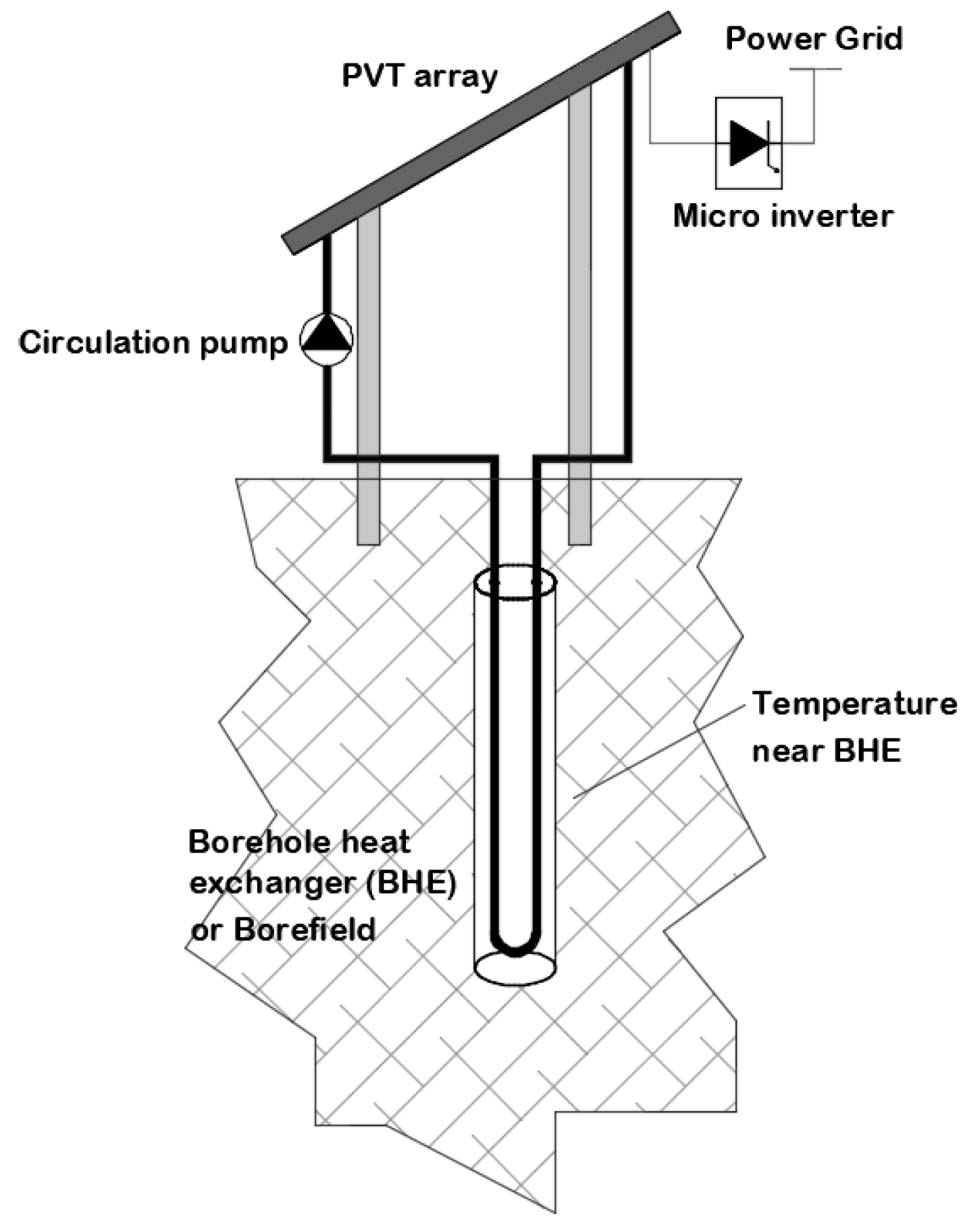
2.1. Set Up of the Assessment

In the current study, a cooling method is evaluated for its potential to increase the electricity yield of PV power plans by reducing the temperature of the cells. The system for evaluation is the PVT collectors to be connected with U-shaped borehole heat exchanger(s) (BHE) (Figure 1). For this purpose, two identical PV panels were installed, and one of them was modified to PVT collector by adding a copper made absorber at its rear side [21]. For both, the PV and the PVT, mathematical models were formulated in TRNSYS [30] (Section 2.3) and validated via experimental data (Section 3.1). The comparison of the PV with the PVT system is carried out for a variety of installed PV capacities and sizes of the GHE. The evaluation is conducted for Athenian (Greece) climatic conditions by utilizing TMY data from Meteonorm. The monthly values of the climatic conditions of Athens useful for the analysis are shown in Figure 2. The simulation span for all cases is set to be 10 years, giving that the system contains GHE which has transient operation during the initial years.

For the PVT systems a small efficient circulation pump (Yonos, Wilo) is considered (Figure 1). The minimum and maximum input power of the pump is 8 to 20 Wp, respectively. Also, the maximum volume flowrate is at 2.7 m³ h⁻¹ and maximum operating pressure is at 10 bars. It is assumed that the pump consumes electricity proportionally related to the flowrate. Thus, the power of the pump is set to 3 W at 1 m³ h⁻¹ to 20 W at 2.7 m³ h⁻¹ (maximum), respectively. It is pertinent to say that the utilized pump increases linearly the power consumption with the flowrate from 0 m³ h⁻¹ to about 1.8 m³ h⁻¹ and adjusts electronically the flowrate and the head. This linear relation between the power and the flowrate is assumed to be acceptable for this study, which is a first approach on the topic, and more in detail analysis can be carried out in the future about the hydraulic part of the system. Thus, for the current study the consumed electricity is not influenced by the number of the PVTs and BHEs, and it is only related to the flow rate. The operation of the circulation pump is dictated by the ΔΤ between the outlet of PVT (s) and the mean soil temperature near BHE (s). For all cases, the ΔΤ should be above 6 K for the circulation pump to start and the irradiance above 5 W m⁻².

Two indices are used for the evaluation of the systems: the percentage fractional improvement (FI), which is illustrated by Equation (1), and the specific productivity (SP) which can be calculated by Equation (2). The FI indicates the percentage improvement on the electrical energy generation of the PVT system compared to the PV one throughout the simulation span. The SP indicates the mean annual electricity (E) or heat (Q) produced per square meter of collector. Of course, the PV system get only SP regarding its electricity (SP_{PV_el}), whereas for the PVT system, the SP can be estimated for its electricity (SP_{PVT_el}) and heat (SP_{PVT_th}) as well. The n in Equation (2) refers to the number of the PVs or PVTs, and the values of E and Q are set to be the total amount of the array, while the A_c stands for the area of the collector. In the case of estimating the SP_{PVT_th} via Equation (2), on the numerator should be placed the Q instead of E.

$$\mathrm{F}\mathrm{I}=100\cdot \frac{{\displaystyle \sum _{\mathrm{i}=\mathrm{y}\mathrm{e}\mathrm{a}\mathrm{r}}^{10}{({\mathrm{E}}_{\mathrm{P}\mathrm{V}\mathrm{T}}-{\mathrm{E}}_{\mathrm{p}\mathrm{u}\mathrm{m}\mathrm{p}}-{\mathrm{E}}_{\mathrm{P}\mathrm{V}})}_{\mathrm{i}}}}{{\displaystyle \sum _{\mathrm{i}=\mathrm{y}\mathrm{e}\mathrm{a}\mathrm{r}}^{10}{\mathrm{E}}_{\mathrm{P}\mathrm{V}}}}$$

(1)

$$\mathrm{S}\mathrm{P}=\frac{{\displaystyle \sum _{\mathrm{i}=\mathrm{y}\mathrm{e}\mathrm{a}\mathrm{r}}^{10}{\mathrm{E}}_{\mathrm{i}}}}{{\mathrm{A}}_{\mathrm{c}}\cdot \mathrm{n}\cdot {10}_{\mathrm{y}\mathrm{e}\mathrm{a}\mathrm{r}\mathrm{s}}}$$

(2)

2.2. Experimental Array

The PV panel and the retrofitted PVT collectors were installed with fixed inclination at 30 degrees and azimuth angle at 25 degrees. The PVT collector is identical to the PV panel (EniTechnologie, Eurosolare75) with the only difference to be the copper made absorber installed at its rear side. The parameters of the PV and PVT are listed in

Table 1. PV and PVT parameters.

PV Panel
Nominal power	76.6 Wp
Nominal efficiency (STC)	14.25%
PV apparatuses area	0.57 m2
Temperature coefficient	0.0046 K−1
Cell type	Polycrystalline (p-Si)
Transmittance Absorptance at normal (τα)n	0.875
Absorber
Type	Serpentine
Material (sheet and tube)	Copper
Distance between pipes (W)	0.064 m
Outer diameter of the tube (Do)	6.35 × 10−3 m
Inter diameter of the tube (Di)	5.35 × 10−3 m
Thickness of the sheet (δ)	3 × 10−4 m
Rear side thermal insulation thickness	1 × 10−2 m
Thermal conductivity the insulation (polyurethane)	4 × 10−2 W m−1 K−1
Bound conductance (Cb)	2 W m−1 K−1

. The experimental array was installed at the University of West Attica in Athens, Greece (former TEI of Athens). It is worth mentioning that results from the current experiment have been published at previous work, with the system to perform during winter weather conditions [21]. For the needs of the present work additional experimentation was conducted during the spring period.

The sketch of the experimental array is illustrated in Figure 3. A small micro inverter was installed at each panel and both were connected to power distribution board. PT100s were used to measure the inlet and outlet temperature of the PVT, the PV’s and PVT’s temperature at the center of the panel (and the ambient temperature as well). The total incident irradiance on the PV and PVT was measured by a CMP 3 Kipp and Zonen pyranometer. Lastly, the wind velocity was measured by a cup-shaped anemometer at 0.1 m above the PV and PVT array. The flow rate was fixed at 0.031 kg s⁻¹ throughout the experimentation. The experimentation day period was set from 10:00 to 17:00, and measurements were logged with 2 min intervals. Measurements were collected and stored by a personal computer from 1/05/2017 to 10/06/2017. The uncertainty of the monitored equipment is listed in

Table 2. Uncertainty of monitored equipment.

Parameter	Nomenclature	Uncertainty
PVT inlet temperature	Tin (°C)	±0.15 °C
PVT outlet temperature	Tout (°C)
PVT absorber temperature (center)	Tpm_PVT (°C)
PV panel temperature (center)	Tpm_PV (°C)
Ambient temperature	Ta (°C)
Incident solar irradiance at tilted surface	GT (W m−2)	±10 W m−2
Wind speed	VW (m s−1)	±0.025 m s−1
PVT and PV power	P (W)	±0.25 W
Flow-rate	m (kg s−1)	±0.001 kg s−1

.

2.3. Mathematical Models

PV and PVT

The mathematical models of PV and PVT are based on the energy balance equation with the purpose of estimating the plate mean temperature (T_{pm_PV} and T_{pm_PVT} for the PV and PVT respectively). Both models (PV and PVT) are iterative by setting an initial guess of the plate mean temperature. It is assumed that the plate mean temperature is equal to the PV cells temperature (T_pm), which directly influence the electrical efficiency (η_e) (Equation (3)). In Equation (3) the η_n is the nominal efficiency of the PV, the β_cell is the temperature coefficient of the PV and the T_STC is the reference temperature (25 °C).

$${\mathsf{\eta }}_{\mathrm{e}}={\mathsf{\eta }}_{\mathrm{n}}[1-{\mathsf{\beta }}_{\mathrm{c}\mathrm{e}\mathrm{l}\mathrm{l}}({\mathrm{T}}_{\mathrm{p}\mathrm{m}}-{\mathrm{T}}_{\mathrm{S}\mathrm{T}\mathrm{C}})]$$

(3)

The generic energy balance equation considers the heat inertia of the PV panel or the PVT collector (panel and absorber, by assuming that the panel, the absorber plate and the water in the tube are all at equal temperature), left side of Equation (4). The heat capacity (MC) of the PV panel was estimated to be 3840 J K⁻¹ and for the PVT collector at 5600 J K⁻¹. On the right side of Equation (4) are the absorbed total solar irradiance (S) multiplied by the PV area (A_c), the produced power (P_e), the produced heat (Q_pr, PVT only), and the heat losses (Q_loss). The differential equation (Equation (4)) was solved via the simple Euler method (Equation (5)) with the aim to estimate the plate mean temperature (T_pm) at each simulation step.

$$(\mathrm{M}\mathrm{C})\frac{\mathrm{d}{\mathsf{{\rm T}}}_{\mathrm{p}\mathrm{m}}}{\mathrm{d}\mathrm{t}}=\mathrm{S}\cdot {\mathrm{A}}_{\mathrm{c}}-{\mathrm{P}}_{\mathrm{e}}-{\mathrm{Q}}_{\mathrm{p}\mathrm{r}}-{\mathrm{Q}}_{\mathrm{l}\mathrm{o}\mathrm{s}\mathrm{s}}$$

(4)

$${\mathrm{T}}_{\mathrm{p}\mathrm{m}}^{\mathrm{i}}=\frac{\mathsf{\Delta }\mathrm{t}}{(\mathrm{M}\mathrm{C})}\cdot (\mathrm{S}\cdot {\mathrm{A}}_{\mathrm{c}}-{\mathrm{P}}_{\mathrm{e}}-{\mathrm{Q}}_{\mathrm{p}\mathrm{r}}-{\mathrm{Q}}_{\mathrm{l}\mathrm{o}\mathrm{s}\mathrm{s}})+{\mathrm{T}}_{\mathrm{p}\mathrm{m}}^{\mathrm{i}-1}$$

(5)

The absorbed irradiance is estimated via Equation (6), where for the incident angle modifier (K_θ) the ASHRAE [32] a single parameter method is adopted (Equation (7)). In Equation (7), the θi is the solar incident angle and the b₀ is the incidence angle modifier coefficient (equal to 0.05). The produce power for both the PV and the PVT is estimated via Equation (8).

$$\mathrm{S}={\mathrm{G}}_{\mathrm{T}}\cdot {(\mathsf{\tau }\mathsf{\alpha })}_{\mathrm{n}}\cdot {\mathrm{K}}_{\mathsf{\theta }}$$

(6)

$${\mathrm{K}}_{\mathsf{\theta }}=1-{\mathrm{b}}_0(\frac{1}{\cos {\mathsf{\theta }}_{\mathrm{i}}}-1)$$

(7)

$${\mathrm{P}}_{\mathrm{e}}={\mathrm{A}}_{\mathrm{c}}\cdot {\mathrm{G}}_{\mathrm{T}}\cdot (\mathsf{\tau }\mathsf{\alpha }{)}_{\mathrm{n}}\cdot {\mathrm{K}}_{\mathsf{\theta }}\cdot {\mathsf{\eta }}_{\mathrm{e}}$$

(8)

Equation (9) estimates the heat losses of the PV or the PVT, where the T_a is the ambient temperature, and the U_L is the overall heat loss coefficient. For the current analysis, the heat loss coefficient is composed of three parts (Equation (10)): the convection heat loss coefficient (h_conv), the front side radiation heat loss coefficient (h_rad), and the heat loss coefficient due to conduction at the rear side of the PVT (this term is applied only for the PVT). The h_conv is calculated by Equation (11), where the coefficient is a linear relation of the wind velocity (V_W). The coefficients were estimated with parameter identification procedure to minimize the RMS error of the model. Thus, for both models (PV and PVT), the slop of the Equation (11) was estimated to be 1.5 and the coefficient C at 8.8 and 26 for the PVT and PV respectively. The radiative heat loss coefficient is estimated via Equation (12), which requires the effective sky temperature (T_sky), which is calculated via Equation (13). In Equation (12), the emissivity (ε_g) is set to 0.95, while the σ stands for the Stefan-Boltzmann constant 5.67 × 10⁻⁸ W m⁻² K⁻⁴. The conduction heat loss coefficient is estimated by the division of the insulation thermal conductivity (λ) by the thickness of the insulation material (δ); both are listed in Table 1.

$${\mathrm{Q}}_{\mathrm{l}\mathrm{o}\mathrm{s}\mathrm{s}}={\mathrm{A}}_{\mathrm{c}}\cdot {\mathrm{U}}_{\mathrm{L}}\cdot ({\mathrm{T}}_{\mathrm{p}\mathrm{m}}-{\mathrm{T}}_{\mathrm{a}})$$

(9)

$${\mathrm{U}}_{\mathrm{L}}={\mathrm{h}}_{\mathrm{c}\mathrm{o}\mathrm{n}\mathrm{v}}+{\mathrm{h}}_{\mathrm{r}\mathrm{a}\mathrm{d}}+{(\frac{\mathsf{\lambda }}{\mathsf{\delta }})}_{\mathrm{c}\mathrm{o}\mathrm{n}\mathrm{d}}$$

(10)

$${\mathrm{h}}_{\mathrm{c}\mathrm{o}\mathrm{n}\mathrm{v}}=1.5\cdot {\mathrm{V}}_{\mathrm{w}}+\mathrm{C}$$

(11)

$${\mathrm{h}}_{\mathrm{r}\mathrm{a}\mathrm{d}}={\mathsf{\epsilon }}_{\mathrm{g}}\mathsf{\sigma }({\mathrm{T}}_{\mathrm{p}\mathrm{m}}^2+{\mathrm{T}}_{\mathrm{s}\mathrm{k}\mathrm{y}}^2)({\mathrm{T}}_{\mathrm{p}\mathrm{m}}+{\mathrm{T}}_{\mathrm{s}\mathrm{k}\mathrm{y}})$$

(12)

$${\mathrm{T}}_{\mathrm{s}\mathrm{k}\mathrm{y}}=0.0552{\mathrm{T}}_{\mathrm{a}}^{1.5}$$

(13)

The heat production of the PVT collectors is calculated via relation 14 [2], where the F_R is the heat removal factor and it is estimated at every simulation time step. It is worth noting that the F_R among many parameters is a function of the flowrate, U_L and the bound conductance of the collector (C_b). In the case of PVT, C_b indicates the thermal conduction between the absorber plate and the pipe of circulated fluid in the absorber. The used PVT is retrofitted from convectional PV panel with a handmade absorber, thus the C_b is poor due to imperfect fitting and is estimated via simulations to be 2 W m⁻¹ K⁻¹ (Equation (15)). Due to serpentine shape of the absorber the F_R is calculated via Equation (15) [33,34].

$${\mathrm{Q}}_{\mathrm{p}\mathrm{r}}={\mathrm{F}}_{\mathrm{R}}\cdot {\mathrm{A}}_{\mathrm{c}}\cdot [\mathrm{S}\cdot (1-{\mathsf{\eta }}_{\mathrm{e}})-{\mathrm{U}}_{\mathrm{L}}\cdot ({\mathrm{T}}_{\mathrm{i}\mathrm{n}}-{\mathrm{T}}_{\mathrm{a}})]$$

(14)

$${\mathrm{F}}_{\mathrm{R}}={\mathrm{F}}_1{\mathrm{F}}_3{\mathrm{F}}_5\left[\frac{2{\mathrm{F}}_4}{{\mathrm{F}}_6\exp [-\sqrt{1-{\mathrm{F}}_2^2/{\mathrm{F}}_3]}+{\mathrm{F}}_5}-1\right]$$

(15)

The parameters F1 through F6 are given by:

$${\mathrm{F}}_1=\frac{\mathrm{k}}{{\mathrm{U}}_{\mathrm{L}}\cdot \mathrm{W}}\cdot \frac{\mathrm{k}\cdot \mathrm{R}(1+\mathsf{\gamma }{)}^2-1-\mathsf{\gamma }-\mathrm{k}\cdot \mathrm{R}}{[\mathrm{k}\cdot \mathrm{R}(1+\mathsf{\gamma })-1{]}^2-{(\mathrm{k}\cdot \mathrm{R})}^2}$$

$${\mathrm{F}}_2=\frac{1}{\mathrm{k}\cdot \mathrm{R}(1+\mathsf{\gamma }{)}^2-1-\mathsf{\gamma }-\mathrm{k}\cdot \mathrm{R}}$$

$${\mathrm{F}}_3=\frac{\mathrm{m}\cdot {\mathrm{c}}_{\mathrm{p}}}{{\mathrm{F}}_1{\mathrm{U}}_{\mathrm{L}}{\mathrm{A}}_{\mathrm{C}}}$$

$${\mathrm{F}}_4={(\frac{1-{\mathrm{F}}_2^2}{{\mathrm{F}}_2^2})}^{1/2}$$

$${\mathrm{F}}_5=\frac{1}{{\mathrm{F}}_2}+{\mathrm{F}}_4-1$$

$${\mathrm{F}}_6=1-\frac{1}{{\mathrm{F}}_2}+{\mathrm{F}}_4$$

$$\mathrm{k}=\frac{(\mathsf{\lambda }\mathsf{\delta }{\mathrm{U}}_{\mathrm{L}}{)}^{1/2}}{\sinh [(\mathrm{W}-{\mathrm{D}}_{\mathrm{o}}){(\frac{{\mathrm{U}}_{\mathrm{L}}}{\mathsf{\lambda }\mathsf{\delta }})}^{1/2}]}$$

$$\mathsf{\gamma }=-2\cosh [(\mathrm{W}-{\mathrm{D}}_{\mathrm{o}}){(\frac{{\mathrm{U}}_{\mathrm{L}}}{\mathsf{\lambda }\mathsf{\delta }})}^{1/2}]-\frac{\mathrm{D}{\mathrm{U}}_{\mathrm{L}}}{\mathrm{k}}$$

$$\mathrm{R}=\frac{1}{{\mathrm{C}}_{\mathrm{b}}}+\frac{1}{\mathsf{\pi }{\mathrm{D}}_{\mathrm{i}}\cdot {\mathrm{h}}_{\mathrm{f}\mathrm{i}}}$$

where in Equation (15), the m and c_p are flowrate and the specific heat capacity of the heat transfer fluid (water), λ and δ are thermal conductivity and the width of the absorber respectively, and h_fi is the in-pipe convection heat transfer coefficient. The in-pipe convection heat transfer coefficient h_fi is calculated via Equations (16) or (17) [34,35] for 0.5 < Pr < 2000. Where in Equations (16) or (17) the index refers to the heat transfer fluid and the μ stands for its dynamic viscosity. Water was used as the heat transfer medium and the utilized thermophysical properties used for the model are listen in

Table 3. Thermophysical properties of water used for the model.

Parameter	Value
Specific heat capacity of the heat transfer fluid, water. (cp)	4185 J kg−1 K−1
Dynamic viscosity of the water (μ)	0.00086 Ns m−2
Water thermal conductivity (λ)	0.56 W m−1 k−1

.

It is worth noting that, in the scientific literature more sophisticated mathematical model for PVs and PVTs than the implemented one can be found [36,37,38,39]. Although for the current study the formulated model which is based on energy balance equation provides acceptable results for long term simulations.

If Re < 2500

$${\mathrm{h}}_{\mathrm{f}\mathrm{i}}=4.36\frac{{\mathsf{\lambda }}_{\mathrm{f}}}{{\mathrm{D}}_{\mathrm{i}}}$$

(16)

or if 2500 < Re < 5,000,000

$${\mathrm{h}}_{\mathrm{f}\mathrm{i}}=(\frac{(\mathrm{f}/8)(\mathrm{Re}-1000)\mathrm{Pr}}{\begin{array}{l}1+12.7(\mathrm{f}/8{)}^{0.5}({\mathrm{Pr}}^{2/3}-1)\\ \mathrm{f}=(0.79\ln \mathrm{Re}-1.64{)}^{-2}\end{array}})\cdot \frac{{\mathsf{\lambda }}_{\mathrm{f}}}{{\mathrm{D}}_{\mathrm{i}}}$$

(17)

where: $\mathrm{Re}=\frac{4\mathrm{m}}{\mathsf{\pi }{\mathrm{D}}_{\mathrm{i}}{\mathsf{\mu }}_{\mathrm{f}}}$ and $\mathrm{Pr}={(\frac{\mathsf{\mu }\cdot {\mathrm{c}}_{\mathrm{p}}}{\mathsf{\lambda }})}_{\mathrm{f}}$.

The accuracy of the model is assessed via the root mean square error (RMSE, Equation (18)) and the mean bias error (MBE, Equation (19)).

$$\mathrm{R}\mathrm{M}\mathrm{S}\mathrm{E}=\sqrt{\frac{{\displaystyle \sum _{\mathrm{i}=1}^{\mathrm{n}}{({\mathrm{Y}}_{\mathrm{s}\mathrm{i}\mathrm{m}}-{\mathrm{Y}}_{\exp })}^2}}{\mathrm{n}}}$$

(18)

$$\mathrm{M}\mathrm{B}\mathrm{E}=\frac{1}{\mathrm{n}}{\displaystyle \sum _{\mathrm{i}=1}^{\mathrm{n}}({\mathrm{Y}}_{\mathrm{s}\mathrm{i}\mathrm{m}}}-{\mathrm{Y}}_{\exp })$$

(19)

Ground heat exchanger

The U-shaped BHE is modeled via TYPE 557 (Hellström’s DST model) of TRNSYS [40]. The BHE’s parameters and thermophysical properties of the soil are listed in

Table 4. BHE’s parameters and thermophysical properties of the soil for Athens.

Parameter	Value
Header depth	0.4 m
Soil thermal conductivity [41]	1.5 W m−1 K−1
Soil (clay) specific heat capacity [41]	2400 kJ m−3 K−1
Soil diffusivity	0.054 m2 day−1
Soil undisturbed temperature [42]	17.2 °C
Grout thermal conductivity (backfill)	1.6 W m−1 K−1
Borehole radius	0.075 m
Outer Radius of Pipe	0.015 m
Inner Radius of Pipe	0.014 m
Pipes center-to-center half distance	0.045 m
Pipe Thermal Conductivity	0.33 W m−1 K−1

. For the parametric analysis of the systems two types of GHE are used, the single BHE (1 to 40 m depth) and borefields. Borefields are comprised of more than one BHE, and for the current study all borefields are very shallow (2 m depth) with spacing between boreholes at 2 m. The TYPE 557 has been used and validated via experimental data for its capacity to estimate the performance of the GHE with very shallow borefield [9]. According to the results, TYPE 557 achieved good agreement with the experimental data, with round mean square error for the outlet temperature of GHE to be 0.67 ± 0.23 °C.

For the validation of single BHE data from Beier et al. [43] were used to validate the TRNSYS TYPE 557. The data are based on experiment conducted via a sandbox. The parameters and properties used by [43] were entered to TYPE 557. Then a simulation was executed in TRNSYS. In Figure 4, simulation results are contrasted with the experimental data, while the GHE outlet temperature was set as the comparative value. As it can be seen, the available data illustrate an interruption on the supplied fluid after 500th min of operation. The mismatch between the model and the data from 500 min to 700 min was due to the limitation of the TYPE 557, which does not consider the heat inertia of the grout. Thus, the outlet temperature dropped abruptly for the model. Measurements are typically recorded once every minute and the model was found capable to follow the restart after about 200 min. Finally, the RMSE% between the results and the offered data was estimated to be 0.75 °C (the value is estimated only for the flowrate existing time).

3. Results and Discussion

3.1. Model Validation

With the purpose to validate the mathematical models of the PV and PVT, five characteristic days are chosen regarding their weather conditions (Figure 5). The weather during the chosen days was varying from the heavily unstable conditions on 12/5 with sporadic rainfalls, 1/6 of which was without abrupt changes.

The performance of the mathematical models was evaluated against the experimental measurements. Both the PV and PVT were evaluated for their capacity to predict the generated power, while the PVT was evaluated for its outlet temperature as well. In Figure 6 and Figure 7 the comparison of the experimentally measured power and this predicted by the models is illustrated for the PV and PVT, respectively. Similarly, in Figure 8 the predicted outlet temperature of the PVT is compared with the experimental one.

As it can be seen, both models can predict the power production via acceptable precision, with RMSE (Equation (18)) to be 2.12 W and 1.76 W for the PV and the PVT, respectively. Similarly, the PVT outlet temperature was predicted accurately with 0.36 °C RMSE. Also, the MBE (Equation (19)) for the produced power was calculated to be 0.88 W and −0.67 W for the PV and the PVT accordingly. Statistically, the model of the PV seems to overestimate the produced power in contrast to that of the PVT which underestimates the produced power. As regards the outlet temperature the MBE was estimated to be 0.17 °C.

Based on the results illustrated in Figure 6 and Figure 7, both models (PV and PVT) are capable of predicting the electrical energy even under heavily unstable weather with rainfalls, such as the period between the 200 and 400 min. Seems that the drops from rainwater on the surface of the panel are not significantly influence its optical characteristics. Thus, the performance of both models regarding the prediction of the electrical energy remained high. At the same transient period (400–800 min, Figure 8), the model of the PVT had the highest deviation from the measured outlet temperature. This was caused due to the inability of the model to assess the heat transfer to the rainwater, which is not consider by the utilized energy balance equation (Equation (4)). Therefore, the solar and ambient energy absorbed by the rainwater is not considered and the Q_pr ends up to be somehow higher, which consequently causes higher outlet temperature.

3.2. Comparison of the Energy Performance

Throughout the carried out comparative studies the assumptions below have been adopted:

• The PV and PVT are scaled up by 3, with the aim to achieve more realistic results. The widely used PV panels have area of about 1.6 m² and this used for the experiment has 0.537 m², about three times smaller. Thus, the used nominal power is set to be 229.8 W, the area (Ac) at 1.611 m² and the MC to be 16,800 J K⁻¹ for the PVT and 11,520 J K⁻¹ for the PV accordingly. The remain parameters are set equal to these listed in Table 1.
• The thermal insulation at the rear side of the PVT is removed and the heat losses due to convection heat losses is estimated via the same Equation (11) and coefficient C as this of the PV (C at 8.8 instead 26 which is for the PVT in Equation (11)). This choice was made in order to maximize the heat losses of PVT by exposing the absorber directly to the ambient conditions, as it applied for the PV panel. It is worth remembering that the convection heat transfer coefficient is related to the temperature difference between the absorber and the adjacent to the absorber air temperature. Thus, the insulated absorber (external side) has low temperature difference from the adjacent air and therefore low heat transfer coefficient. Though the naked PVT with the copper made absorber has higher temperature difference with the adjacent air, thus higher heat transfer coefficient. In reality, the naked absorber may have higher heat transfer coefficient even from the PV, which has at its rear side EVA, but for the current study we can set these values to be equal.

3.2.1. Parametric Analysis of a Single PVT Collector

The illustrated results of this section are estimated from a ten-year simulation period and by using hourly values of a typical meteorological year. The main climatic data of the TMY are shown in Figure 2. The first analysis is carried out by comparing 1 PV with 1 PVT paired with very shallow GHE (Figure 1). The comparison is conducted by varying the flowrate from 20 kg h⁻¹ to 200 kg h⁻¹ and the number of BHEs from one to four, the results are illustrated in Figure 9. As it can be seen, the PVT outperforms the PV in all of the scenarios. The specific productivity of the PV (SP_{PV_el}) was estimated to be slightly less than 202 kWh_e m⁻² and this of the PVT (SP_{PVT_el}) was varied from about 210.7 kWh_e to 214 kWh_e m⁻² for the highest flowrate (200 kg h⁻¹) with 1 BHEs to the lowest flowrate (20 kg h⁻¹) with 4 BHEs, respectively. The SP_{PVT_el} increases as the geothermal heat exchanger enlarges due to higher heat capacity of the soil. With high heat capacity (more soil mass) and for a given amount of thermal energy, the mean temperature of the soil will increase less than a smaller borefield (

Table 5. Fractional improvement for one PVT paired with one to four BHEs. All BHEs are at 2 m vertical length and with 2 m spacing.

Flowrate (kg/h)	Fractional Improvement, FI (%)				Soil Temperature near BHEs (°C)
	1 BHE	2 BHE	3 BHE	4 BHE	1 BHE	2 BHE	3 BHE	4 BHE
20	0.49	0.95	1.34	1.71	24.03	23.92	23.67	23.53
40	0.45	0.85	1.22	1.55	23.96	23.74	23.35	23.14
60	0.54	0.88	1.21	1.48	23.84	23.57	23.15	22.89
80	0.80	1.17	1.43	1.67	23.61	23.32	22.90	22.65
100	1.19	1.48	1.69	1.89	23.16	22.90	22.52	22.29
120	1.70	1.82	1.98	2.17	22.38	22.23	21.94	21.75
140	2.11	2.23	2.36	2.42	21.41	21.34	21.11	21.04
160	2.37	2.47	2.52	2.62	20.49	20.46	20.38	20.28
180	2.53	2.59	2.61	2.66	19.93	19.91	19.90	19.80
200	2.50	2.58	2.59	2.67	19.86	19.72	19.72	19.58

). With lower soil temperature, the solar heat is transferred more frequently, since the possibility to achieve a ΔT of 6 K between the PVTs and the soil is increased. Furthermore, the electric specific productivity of the PVT was found to drop as the flowrate increase. The higher flowrate causes lower PVT outlet temperature, thus the occasions to achieve the conditions for the solar heat to be transferred into the ground are reduced.

In Table 5 the percentage fractional improvement (FI) (Equation (1)) of one PVT collector against one PV is listed as function of the flowrate and the number of BHEs (Figure 1). The FI was found to increase as the flowrate rise, even though the electric specific productivity of the PVT found to drop accordingly. In details, the FI was found from 0.49 to 2.67%, for one BHE and four BHEs and with the lowest and the highest flowrate, respectively. The improvement of the FI with higher flowrates is due to the reduced electricity consumed by the circulation pump. The operation of the pump was constrained by the lower PVT outlet temperature, which consequently reduce the possibility for heat transfer from the collector into the ground. This can be explained via Figure 10, where the plate mean temperature of the PV, PVT, and the soil’s temperature are shown as function of the flowrate for the scenario of four BHEs. As it can be seen, the plate mean temperature of the PVT rises as the flowrate increases. This was caused by the less frequently used circulation pump. Thus, less heat was removed from the PVT, and consequently the efficiency of the PV-cells was reduced (Figure 1). It is worth noting that the soil’s temperature near BHEs was affected also by the pump’s reduced operation. As a result, the mean soil temperature near boreholes was found to drop from 24 °C to 20 °C for the scenarios of flowrates between 20 kg h⁻¹ and 200 kg h⁻¹, respectively. Also, the annual operation hours of the circulation pump were found to fall with similar trend as this of the soil temperature. The annual hours of the pump’s operation were found to be from about 2300 h to 1000 h for the lowest and the highest flowrate accordingly.

3.2.2. Balance of the Soil Temperature

One of the remaining questions is whether the geothermal part of the proposed system remains stable during the period of analysis. In particular, if the temperature of the soil increases steadily and if the operation of the system is defected for this. For pure solar system one-year performance analysis is substantial to provide the overview regarding its energy performance, but this is not the case for systems with GHE. In Figure 11 the soil temperature near BHEs is shown for a 10-year simulation period and for a system of four PVTs (in series connected) with two BHEs (2 m deep and 2 m spacing). As it can be seen the mean soil temperature increase smoothly from 16.4 °C to 17.4 °C within the initial-period of six years, and after that transient period the mean temperature remains stable. Given that, the operation of the system is not influenced significantly, while the initial and steady state conditions of the soil can be considered during the design stage. Throughout the executed simulations of this study, the soil temperature illustrates this behavior, increases by 1 °C to 2 °C within the first six years of simulation and then remains stable.

3.2.3. Influence of the BHE Length and Size

The influence of the BHE’s length on the energy performance of the system is illustrated by

Table 6. Simulation results as function of the a single BHE with vertical length from 1 to 40 m. For 1 PVT with flowrate of 80 kg h⁻¹. *, average annual plate mean temperature of the PV and PVT. **, mean soil temperature near BHEs.

Length of BHE (m)	SPPV_el (kWh m−2)	SPPVT_el (kWh m−2)	SPPVT_th (kWh m−2)	Pump Consumption (kWh)	FI (%)	Tpm_PV * (°C)	Tpm_PVT * (°C)	Tsoil ** (°C)
1	201.7	210.7	43.6	12.4	0.61	23.9	21.7	23.8
2	201.7	211.2	91.1	12.6	0.80	23.9	21.5	23.6
4	201.7	212.2	187.3	13.2	1.12	23.9	21.2	23.2
6	201.7	213.1	281.8	13.9	1.36	23.9	20.8	22.7
10	201.7	214.6	452.0	14.9	1.80	23.9	20.3	21.8
15	201.7	216.1	627.5	16.3	2.15	23.9	19.7	20.9
20	201.7	217.3	774.6	17.1	2.47	23.9	19.2	20.1
25	201.7	218.3	891.7	17.9	2.74	23.9	18.8	19.4
30	201.7	219.0	989.0	18.3	2.93	23.9	18.4	18.9
40	201.7	220.1	1138.2	18.9	3.30	23.9	17.9	18.0

. For this analysis the vertical length of the BHE varies from 1 to 40 m, and this is connected with a single PVT collector with 80 kg h⁻¹ flowrate. According to the results, the electric specific productivity of the PVT was higher than this of the PV through all the lengths of the BHE. By setting as benchmark the SP of the PV (201.7 kWh m⁻²), the SP_{PVT_el} was estimated from 210.7 to 220.1 kWh m⁻² for the shortest and the longest BHE respectively. The improvement on the SP_{PVT_el} was caused by the lower plate mean temperature (PV cell) due to the solar heat transfer from the collector into the ground. As it can be seen in Table 6, the mean annual T_{pm_PV} was estimated to be 23.9 °C and the mean annual T_{pm_PVT} was found from 21.7 °C to 17.9 °C with the BHE of 1 m and 40 m respectively. The reduced T_{pm_PVT} augments the electrical performance of the cells. The heat specific productivity of the PVT increases as the length of the BHE enlarges for two reasons: (a) the larger heat transfer area which is provided by a larger BHE, and (b) due to lower mean annual soil temperature which can be reached at greater depths, in particular during summer where the close to ground surface soil mass is heated up. This is depicted by the values listed in Table 6 where for the shortest BHE (1 m) the SP_{PVT_th} is 43.6 kWh m⁻² and for the longest BHE this value is increased at 1138.2 kWh m⁻². It is important to state that the annual total incident irradiation is 1708 kWh m⁻².

Figure 12 is printed with the aim to illustrate how the in-series hydraulic connection of the PVTs influence their energy performance (the outlet of the first is the inlet of the second and so on). Figure 12 shows the plate mean temperature of the PVT array as function of one string consisted of one to eight collectors in series (the illustrated value is the average out of all connected PVTs). The evaluation is made by considering four different types of geothermal heat exchangers, a borefield of 4 BHEs at 2 m depth and 2 m spacing, and a single BHE with three vertical lengths (10, 20, and 40 m). Along with the plate mean temperatures, the fractional improvement is illustrated for all simulation scenarios (Equation (1)). As it is expected, the plate mean temperature rises as the number of the in-series collectors increase and reach a plateau after a certain number of collectors. In details, for the borefield of four very shallow BHEs and for the BHE of 10 m depth the plate mean temperature stagnates at the fourth PVT, while for 20 m BHE the stagnation is achieved after the seventh PVT. The BHE of 40 m does not reach a plateau at any number of PVTs, and more collectors connected in-series are required for the stagnation. The BHEs of 40 m does not level the T_pm due to the larger soil mass adjacent to the borehole, which requires more PVTs in-series to stagnate. It is important to note that for the current analysis the in parallel connection of PVT is not evaluated, and the aim is to find out the influence of the in-series connection.

The fractional improvement for all cases (geothermal heat exchangers) rises and then reaches a plateau or reduces slightly (Figure 12). It is worth noting that the FI increases substantial from the single PVT to the array of 2 PVTs. In particular the FI for the borefield (4 BHEs) rises from slightly less than 2 to 4% by just adding one more collector. The improvement on the FI is made due to the higher outlet temperature of the array which has greater potential to transfer the solar heat into the ground. For the borefield and the BHE of 10 m the FI levels at the 4th PVT, though for the remaining BHEs the FI drops slightly as the number of PVTs increase. This is caused by the continuously increasing plate mean temperature (upper figure, Figure 12) which reduces the electrical efficiency of the PV cells. Based on the results, for all investigated geothermal heat exchangers there is a certain number connected in-series PVTs wherein the system achieves the higher FI. After this point the FI remains stable for the smaller geothermal heat exchanger or reduces for the larger ones.

3.2.4. PVT Array and Borefield Size Parametric Analysis

The very shallow borefields with less than 2 m depth are in particular interest, since they can be built with a small drilling rig. This can improve the economy of the systems by reducing the costs correlated to the construction of the geothermal heat exchanger [44] and the construction time. With this particular interest, Figure 13 illustrates the electric and heat specific productivity for three PVT array sizes (4, 8, and 12 PVTs) and six borefield sizes (4, 8, 12, 16, 20, and 24 BHEs). Two distinctive trends are illustrated in Figure 13, the electric and heat SP increase as the borefield enlarges and reduce as the array enlarges. As the borefield enlarges more heat transfer area is available (BHEs) and more adjacent soil volume, and these increase the SP (heat and power). In contrast, as the PVT array enlarges more solar heat is transferred into the ground and that elevates the temperature of the soil (Figure 14). The higher soil temperature ends up to higher inlet temperature for the PVT array, and it is well known the electric and thermal efficiency of the collector reduce as the inlet temperature rises. It is pertinent to note that the produced heat is not used and is diffused naturally to the adjacent soil masses and surface. If the heat from the soil was remove in order to cover a heating load (industry, space heating etc.), the productivity of the system will improve due to the dropped soil temperature.

Figure 14 is based on the results as these of Figure 13 and illustrates the annual solar heat transferred to the soil per meter of BHE (upper figure) and the mean annual soil temperature near BHEs. As it can be seen, the heat per meter BHE reduces as the borefield enlarges, since for the same amount of heat (from PVTs) more BHEs are available. In details, the annual heat per meter of BHE was estimated to be from 63 to 78 kWh per meter of BHE, for the array of 4 and 12 PVTs, respectively. A benchmark can be established from the illustrated results, regarding the annual heat transfer potential of the borefield, which for the given analysis is about 70 kWh m⁻¹. The mean annual soil temperature (bottom figure, Figure 14) varies from 23.8 °C to 22.3 °C, for the smallest and the largest borefield accordingly.

3.2.5. Variation of the Soil Temperature near BHEs

The annual variation of the soil near BHEs is shown in Figure 15 for the borefields of 4, 12, and 24 BHEs paired with 4 PVTs in contrast to the natural soil temperature (no system). All temperatures are illustrated at 1.5 m depth. All temperatures follow the same trend, which is lower values during winter months and the peak values during summer and especially on August. The natural soil temperature gets its maximum value one month later on September. It is worth noting that the soil temperature near BHEs is about 8–10 °C higher than the natural temperature during the season with the highest available solar energy (May to September, Figure 2). This temperature difference between the system made and the natural condition depicts the potential for further improvement of the systems energy performance. In other words, the lower the soil temperature near BHEs, the higher the electric SP. That highlights the need to remove the solar heat stored into the ground during the summer months in order to enhance the electrical energy generation.

3.2.6. Comparison of the Results with the Existing Literature

Based on the results, the single PVT collector can achieve FΙ of 2.67% and 3.30% for the borefield of 4 BHEs and the BHE of 40 m depth, respectively (Table 5 and Table 6). With the very shallow borefield of 4 BHEs paired with the array of 4 PVTs (connected in series) the FI was estimated to be 4% (Figure 12). The highest value of FI estimated from the study is at 5.5% for the array of 3 PVTs and the BHE of 40 m depth (Figure 12). In

Table 7. Summary of the methods found in the existing literature about the improvement of the PV cell efficiency by utilizing PVT collectors. The listed fractional improvements illustrate values estimated via a certain time period (instantaneous, hourly, daily FI).

Work	System	FI (%)
Experiment [16]	Open loop air-based PVT systems (Singapore)	12–14
Experiment [17]	Open loop air-based PVT systems (Sydney, Australia)	10.6–12.2
Experiment andSimulations [22]	Water based PVT with horizontal GHE of 80 m buried 3 m (North-West India)	1.02–1.41
Experiment (Indoor) [24]	Water based PVT system with serpentine shaped absorber (Indoor)	3
Experiment [25]	Water based PVT with microchannel pair with a spiral shaped GHE (3 depth) (Ankara, Turkey)	10
Experiment and imulations [20]	Water bases PVT system with water tank (Dhahran, Saudi Arabia)	9
Experiment [21]	Water bases PVT system with water tank (Athens, Greece)	0.32

are listed the main findings for the existing literature, regarding the methods which can be used to improve the PV cell efficiency by the means of PVT collectors. It is important to note that the current analysis is to set the findings in the winder picture, since the results are derived from different climatic conditions, systems layout, PV nominal efficiency and so forth. Also, the results from the current study are about the annual FI while the values listed in Table 7 are estimated for shorter time periods.

3.2.7. Capital Cost of the Investigated System

After consultation with industry, the capital cost per installed kW_p of the proposed system breaks down to: the cost for PVT absorbers (180–240 € per kW_p), the circulation pump cost (40–70 € per kW_p) and the BHE cost per meter of BHE (70–90 € per m of BHE). Based on the above stated prices and the system with 4 PVTs and the 4BHEs (Figure 12), the initial cost of the system per installed kW_p varies from 680 € to 1030 €. This investment can offer about 3.8% more electricity yield than a conventional PV system (Figure 12). Here we can provide the current price for two axes tracker systems which is from 900 to 1300 € per kW_p. The stated capital costs are about to provide the magnitude of the investigated system in contrast to an established technology (two axes tracking). The comparison on the capital costs refers to the Greek market only and a rigorous economic analysis is required for obtaining accredited results.

4. Conclusions

In the present work, a PVT—geothermal system is evaluated regarding its capacity to increase the annual generated electricity contrary to a conventional PV system. Experimentation was carried out with a PV and PVT collector in Athens (Greece), with the aim to collect data for the validation of the models. The models of the PV and PVT were formulated in TRNSYS and validated. With the built models, simulation based parametric analyses were contacted by varying the size of the PV and PVT array, the flowrate, and the size of the geothermal heat exchanger (GHE) as well.

Both models of the PV and PVT are capable of estimating the production of the electrical energy. With more details, the RMS error regarding the electricity was calculated to be 2.12 W and 1.76 W for the PV and the PVT, respectively. The RMS error for the temperature outlet of the PVT was estimated to be 0.36 °C. Additionally, both models illustrate the capability of following transient weather conditions, with the only inadequacy for the PVT being the ability to estimate the outlet temperature during raining weather.

The percentage fractional improvement (FI) estimated via the implementation of the PVT-shallow geothermal system varies from 0.61 to 5.5% for the shortest borehole heat exchanger (BHE) of 1 m and the longest of 40 m, respectively. The estimated FI values of the current work are at the same magnitude with this illustrated by the existing literature, from 1% up to 10%. The electric annual specific productivity (SP) for PV was estimated to be about 202 kWh m⁻² and for the base case scenario of 4 PVTs paired with 4 BHEs (2 m depth) to be 213 kWh m⁻². It is important to highlight that the proposed system outperforms energetically the conventional PV system even with the smaller BHE of 1 m paired with 1 PVT collectors. Furthermore, the FI and SP are two indices which can be used for the evaluation of the systems, and the FI can illustrate the overall performance. Through the FI the importance of very efficient circulation pump is shown. The electric SP of the PVT was found to increase as the GHE enlarges and to decrease as the flowrate rises. Also, as the flowrate increases the outlet temperature of the PVT reduces and this reduction drops the potential for heat transfer to the ground.

Throughout all parametric analyses, the annual mean soil temperature was found to reach a steady state value after the fifth year of operation. Also, a significant enhancement on the FI was found by increasing the number of the PVT collectors connected in series. A distinctive different between the mean soil temperature caused by the systems was found against the natural temperature of the soil. This temperature difference is estimated to be about 8 °C during the summer months. It is a good practice to investigate methods with the aim to reduce the soil temperature during summer, and by that to increase the electric SP of the system. The connection of the proposed system with heating loads may be a way to remove heat from the soil and by that to utilize the produced heat.

References

1. Wolf, M. Performance analyses of combined heating and photovoltaic power systems for residences. Energy Convers 1976, 16, 79–90. [Google Scholar] [CrossRef]
2. Florschuetz, L. Extension of the Hottel-Whillier Model to the Analysis of Combined Photovoltaic/Thermal Flat Plate Collectors. Sol. Energy 1979, 22, 361–366. [Google Scholar] [CrossRef]
3. Chow, T.T. A review on photovoltaic/thermal hybrid solar technology. Appl. Energy 2010, 87, 365–379. [Google Scholar] [CrossRef]
4. Ibrahim, A.; Othman, M.Y.; Ruslan, M.H.; Mat, S.; Sopian, K. Recent advances in flat plate photovoltaic/thermal (PV/T) solar collectors. Renew. Sustain. Energy Rev. 2011, 15, 352–365. [Google Scholar] [CrossRef]
5. Aste, N.; del Pero, C.; Leonforte, F. Water flat plate PV-thermal collectors: A review. Sol. Energy 2014, 102, 98–115. [Google Scholar] [CrossRef]
6. Debbarma, M.; Sudhakar, K.; Baredar, P. Comparison of BIPV and BIPVT: A review. Resour. Technol. 2017, 3, 263–271. [Google Scholar] [CrossRef]
7. Sommerfeldt, N.; Madani, H. Review of Solar PV/Thermal Plus Ground Source Heat Pump Systems for European Multi-Family Houses. In Proceedings of the EuroSun Conference, Palma de Mallorca, Spain, 11–14 October 2016; pp. 1–12. [Google Scholar]
8. Nouri, G.; Noorollahi, Y.; Yousefi, H. Solar assisted ground source heat pump systems—A review. Appl. Therm. Eng. 2019, 163. [Google Scholar] [CrossRef]
9. Sakellariou, E.I.; Wright, A.J.; Axaopoulos, P.; Oyinlola, M.A. PVT based solar assisted ground source heat pump system: Modelling approach and sensitivity analyses. Sol. Energy 2019, 193, 37–50. [Google Scholar] [CrossRef]
10. De Soto, W.; Klein, S.A.; Beckman, W.A. Improvement and validation of a model for photovoltaic array performance. Sol. Energy 2006, 80, 78–88. [Google Scholar] [CrossRef]
11. Dubey, S.; Sarvaiya, J.N.; Seshadri, B. Temperature dependent photovoltaic (PV) efficiency and its effect on PV production in the world—A review. Energy Procedia 2013, 33, 311–321. [Google Scholar] [CrossRef] [Green Version]
12. Zondag, H. Flat-plate PV-Thermal collectors and systems: A review. Renew. Sustain. Energy Rev. 2008, 12, 891–959. [Google Scholar] [CrossRef] [Green Version]
13. Maleki, A.; Haghighi, A.; El Haj Assad, M.; Mahariq, I.; Alhuyi Nazari, M. A review on the approaches employed for cooling PV cells. Sol. Energy 2020, 209, 170–185. [Google Scholar] [CrossRef]
14. Good, C.; Andresen, I.; Hestnes, A.G. Solar energy for net zero energy buildings—A comparison between solar thermal, PV and photovoltaic-thermal (PV/T) systems. Sol. Energy 2015, 122, 986–996. [Google Scholar] [CrossRef] [Green Version]
15. Fuentes, M.; Vivar, M.; de la Casa, J.; Aguilera, J. An experimental comparison between commercial hybrid PV-T and simple PV systems intended for BIPV. Renew. Sustain. Energy Rev. 2018, 93, 110–120. [Google Scholar] [CrossRef]
16. Teo, H.G.; Lee, P.S.; Hawlader, M.N.A. An active cooling system for photovoltaic modules. Appl. Energy 2012, 90, 309–315. [Google Scholar] [CrossRef]
17. Bambrook, S.M.; Sproul, A.B. Maximising the energy output of a PVT air system. Sol. Energy 2012, 86, 1857–1871. [Google Scholar] [CrossRef]
18. Krauter, S. Increased electrical yield via water flow over the front of photovoltaic panels. Sol. Energy Mater. Sol. Cells 2004, 82, 131–137. [Google Scholar] [CrossRef]
19. Kordzadeh, A. The effects of nominal power of array and system head on the operation of photovoltaic water pumping set with array surface covered by a film of water. Renew. Energy 2010, 35, 1098–1102. [Google Scholar] [CrossRef]
20. Bahaidarah, H.; Subhan, A.; Gandhidasan, P.; Rehman, S. Performance evaluation of a PV (photovoltaic) module by back surface water cooling for hot climatic conditions. Energy 2013, 59, 445–453. [Google Scholar] [CrossRef]
21. Sakellariou, E.; Axaopoulos, P. Simulation and experimental performance analysis of a modified PV panel to a PVT collector. Sol. Energy 2017, 155, 715–726. [Google Scholar] [CrossRef]
22. Jakhar, S.; Soni, M.S.; Gakkhar, N. An integrated photovoltaic thermal solar (IPVTS) system with earth water heat exchanger cooling: Energy and exergy analysis. Sol. Energy 2017, 157, 81–93. [Google Scholar] [CrossRef]
23. Elminshawy, N.A.S.; El Ghandour, M.; Gad, H.M.; El-Damhogi, D.G.; El-Nahhas, K.; Addas, M.F. The performance of a buried heat exchanger system for PV panel cooling under elevated air temperatures. Geothermics 2019, 82, 7–15. [Google Scholar] [CrossRef]
24. Ariff, W.; Bin, F.; Abdullah, W.; Ping, C.S.; Binti, R.N. The Improvement on the Efficiency of Photovoltaic Module using Water Cooling. OP Conf. Ser. Earth Environ. Sci. 2021, 721, 012001. [Google Scholar] [CrossRef]
25. Jafari, R.; Erkılıç, K.T.; Uğurer, D.; Kanbur, Y.; Yıldız, M.; Ayhan, E.B. Enhanced photovoltaic panel energy by minichannel cooler and natural geothermal system. Int. J. Energy Res. 2021, 1–11. [Google Scholar] [CrossRef]
26. Awasthi, A.; Shukla, A.K.; Murali Manohar, S.R.; Dondariya, C.; Shukla, K.N.; Porwal, D.; Richhariya, G. Review on sun tracking technology in solar PV system. Energy Rep. 2020, 6, 392–405. [Google Scholar] [CrossRef]
27. Nsengiyumva, W.; Chen, S.G.; Hu, L.; Chen, X. Recent advancements and challenges in Solar Tracking Systems (STS): A review. Renew. Sustain. Energy Rev. 2018, 81, 250–279. [Google Scholar] [CrossRef]
28. Fernández-Ahumada, L.M.; Casares, F.J.; Ramírez-Faz, J.; López-Luque, R. Mathematical study of the movement of solar tracking systems based on rational models. Sol. Energy 2017, 150, 20–29. [Google Scholar] [CrossRef]
29. Racharla, S.; Rajan, K. Solar tracking system–a review. Int. J. Sustain. Eng. 2017, 10, 72–81. [Google Scholar] [CrossRef]
30. Solar Energy Laboratory University of Wisconsin-Madison, GmbH—TRANSSOLAR Energietechnik, CSTB—Centre Scientifique et Technique du Bâtiment, TESS—Thermal Energy Systems Specialists. TRNSYS 17—a TRaNsientSYstem. Simulation Program. Simulation, 2009.
31. Meteonorm. Irradiation Data for Every Place on Earth; Solar Energy Laboratory, University of Wisconsin: Madison, WI, USA, 2016. [Google Scholar]
32. ASHRAE. Methods of Testing to Determine the Thermal Performance of Solar Collectors; ASHRAE: Peachtree Corners, GA, USA, 1977; pp. 93–97. [Google Scholar]
33. Zhang, H.F.; Lavan, Z. Thermal Performance of a Serpentine Absorber Plate. Proc. Annu. Meet. Am. Sect. Int. Sol. Energy Soc. 1983, 34, 471–476. [Google Scholar] [CrossRef]
34. Duffie, J.A.; Beckman, W.A. Solar Engineering of Thermal Processes, 4th ed.; Wiley: Hoboken, NJ, USA, 2013. [Google Scholar]
35. Incropera, F.P.; DeWitt, D.P.; Bergman, T.L.; Lavine, A.S. Heat and mass transfer—Incropera 6e. Fundam. Heat. Mass. Transf. 2007, 997. [Google Scholar] [CrossRef]
36. Dolara, A.; Leva, S.; Manzolini, G. Comparison of different physical models for PV power output prediction. Sol. Energy 2015, 119, 83–99. [Google Scholar] [CrossRef] [Green Version]
37. Ventura, C.; Tina, G.M.; Gagliano, A.; Aneli, S. Enhanced models for the evaluation of electrical efficiency of PV/T modules. Sol. Energy 2021, 224, 531–544. [Google Scholar] [CrossRef]
38. El Fouas, C.; Hajji, B.; Gagliano, A.; Tina, G.M.; Aneli, S. Numerical model and experimental validation of the electrical and thermal performances of photovoltaic/thermal plant. Energy Convers. Manag. 2020, 220, 112939. [Google Scholar] [CrossRef]
39. Maadi, S.R.; Khatibi, M.; Ebrahimnia-Bajestan, E.; Wood, D. Coupled thermal-optical numerical modeling of PV/T module—Combining CFD approach and two-band radiation DO model. Energy Convers. Manag. 2019, 198, 111781. [Google Scholar] [CrossRef]
40. Hellström, G. Duct Ground Heat Storage Model, Manual for Computer Code. Energy 1989. [Google Scholar]
41. Technical Chamber of Greece. Technical Directive 20701-1: National Specifications of Parameters for Calculating the Energy Performance of Buildings and the Issue of the Energy Performance Certificate 2017; Technical Chamber of Greece: Athens, Greece, 2017. [Google Scholar]
42. Badache, M.; Eslami-Nejad, P.; Ouzzane, M.; Aidoun, Z.; Lamarche, L. A new modeling approach for improved ground temperature profile determination. Renew. Energy 2016, 85, 436–444. [Google Scholar] [CrossRef]
43. Beier, R.A.; Smith, M.D.; Spitler, J.D. Reference data sets for vertical borehole ground heat exchanger models and thermal response test analysis. Geothermics 2011, 40, 79–85. [Google Scholar] [CrossRef]
44. Sakellariou, E.I.; Axaopoulos, P.J.; Wright, A.J. Energy and economic evaluation of a solar assisted ground source heat pump system for a north Mediterranean city. Energy Build. 2020, 231, 110640. [Google Scholar] [CrossRef]
Figure 1. Generic layout of the PVT-BHE system.
Energies 14 06415 g001
Figure 2. Monthly values for Athens (Greece) of the ambient temperature, natural soil temperature at 2 m depth, total solar irradiation on tilted surface with inclination 30° and azimuth of 0°, along with the mean monthly value of the wind velocity [31].
Energies 14 06415 g002
Figure 3. Sketch of the experimental array.
Energies 14 06415 g003
Figure 4. GHE outlet fluid temperature comparison between data resourced by [43] and TYPE 557.
Energies 14 06415 g004
Figure 5. Important weather parameters of the five chosen days for the validation of the PV and PVT models. The incident irradiance on the surface is for inclination 30° and azimuth 25°.
Energies 14 06415 g005
Figure 6. Power production of the PV, model prediction against experimental data. For the total of five days (from 10:00 to 17:00).
Energies 14 06415 g006
Figure 7. Power production of the PVT, model prediction against data. For the total of five days (from 10:00 to 17:00). The flowrate was fixed to 111.6 kg h−1.
Energies 14 06415 g007
Figure 8. PVT’s outlet temperature, model prediction against data. For the total of five days (from 10:00 to 17:00). The flowrate was fixed to 111.6 kg h−1.
Energies 14 06415 g008
Figure 9. Electric specific productivity (SP) of one PV and of one PVT connected with one to four BHEs (four scenarios). All BHEs are in 2 m depth and with 2 m spacing.
Energies 14 06415 g009
Figure 10. Upper figure, plate mean (pm) temperature of the PVT, PV, and the mean annual soil temperature near BHEs as function of the flowrate. For all scenarios one PV and one PVT are used, paired with four BHEs with 2 depth and 2 m spacing. The bottom figure illustrates the total operation hours of the circulation pump.
Energies 14 06415 g010
Figure 11. Mean temperature near BHEs and mean annual temperature near BHEs for 10-year simulation span, for a system with four PVTs and four BHEs (2 m deep and 2 m spacing).
Energies 14 06415 g011
Figure 12. Upper figure, plate mean temperature (Tpm) of the PV and PVT for a variety of GHE (10-year simulation). The Tpm is illustrated as function of the PVTs connected in series hydraulically and depicts the average value out of all collectors, electrically are all connected with microinverters (no strings). Bottom figure, the fractional improvement for all studied scenarios of GHE as function of the PVTs connected in series. The flowrate for all cases is 80 kg h−1.
Energies 14 06415 g012
Figure 13. Electric and heat specific productivity of the PV and PVTs, as function of the size PVT array (4, 8, and 12 PVTs) and the number of the BHEs (4, 8, 12, 16, 20, and 24 BHE) (10-year simulation). The PVT arrays are formulated with strings of four collectors in series similarly the borefield are shaped with 4 BHEs connected in series (hydraulically). All borefields consist of BHE with 2 m vertical length and 2 m spacing. For each string the flowrate is set to be 80 kg h−1.
Energies 14 06415 g013
Figure 14. Upper figure, annual heat transferred into the ground per meter of BHE as function of the PVT array and of the borefield size (10-year simulation). Bottom figure, soil temperature near BHEs as function of the PVT array and of the borefield size. The PVT arrays are formulated with strings of four collectors in series similarly the borefield are shaped with 4 BHEs connected in series (hydraulically). All borefields are consisted of BHE with 2 m vertical length and 2 m spacing. For each string the flowrate is set to be 80 kg h−1.
Energies 14 06415 g014
Figure 15. Annual variation of the soil temperature near BHEs at 1.5 m depth for three borefields, 4, 12, and 24 BHEs connected with a 4 PVTs. The near BHEs temperatures are contrasted with the natural soil temperature at 1.5 m (without system). All BHEs assumed to be 2 m deep and 2 m spacing, the array of 4 PVTs are in series connected hydraulically.
Energies 14 06415 g015