1. Introduction
In the European Union (EU), residential and non-residential buildings account for 75% and 25% of the total building stock, respectively [
1]. Office buildings have a significant share of 23% among non-residential buildings stock, which is considered a viable source of energy usages [
1]. For instance, the average heating and cooling need of office buildings in the EU are 159 and 7 TWh/year, respectively [
2]. Though these are the key sectors of energy use in buildings, significant variations of heating and cooling need are observed when buildings are located in different climates. To fulfil the same thermal comfort and other indoor environmental quality (IEQ) criteria, different outdoor conditions will cause substantial differences in energy demands for heating, cooling, ventilation, and lighting. Thus, the EU defines the benchmark of nearly zero energy building (NZEB) office building for four climate zones [
3].
Many scientific research works introduce building parameters and their uncertainties, which have significant impacts on buildings’ energy efficiency [
4,
5,
6]. Eisenhower et al. [
4] presented a large number of potential parameters that have a substantial effect on buildings design. Bucking et al. [
5] proposed a methodology in which scaling up the different building parameters for improving buildings’ energy efficiency. Besides, this study distinguished the effects of insulation level and window areas on buildings’ energy performance. In the same context, Sun et al. [
6] analyzed the uncertainty of microclimatic variables, namely local temperature, solar irradiation, wind speed, and pressure for the energy assessment of buildings. The study showed the fundamental differences in energy consumption due to climatic variations [
6].
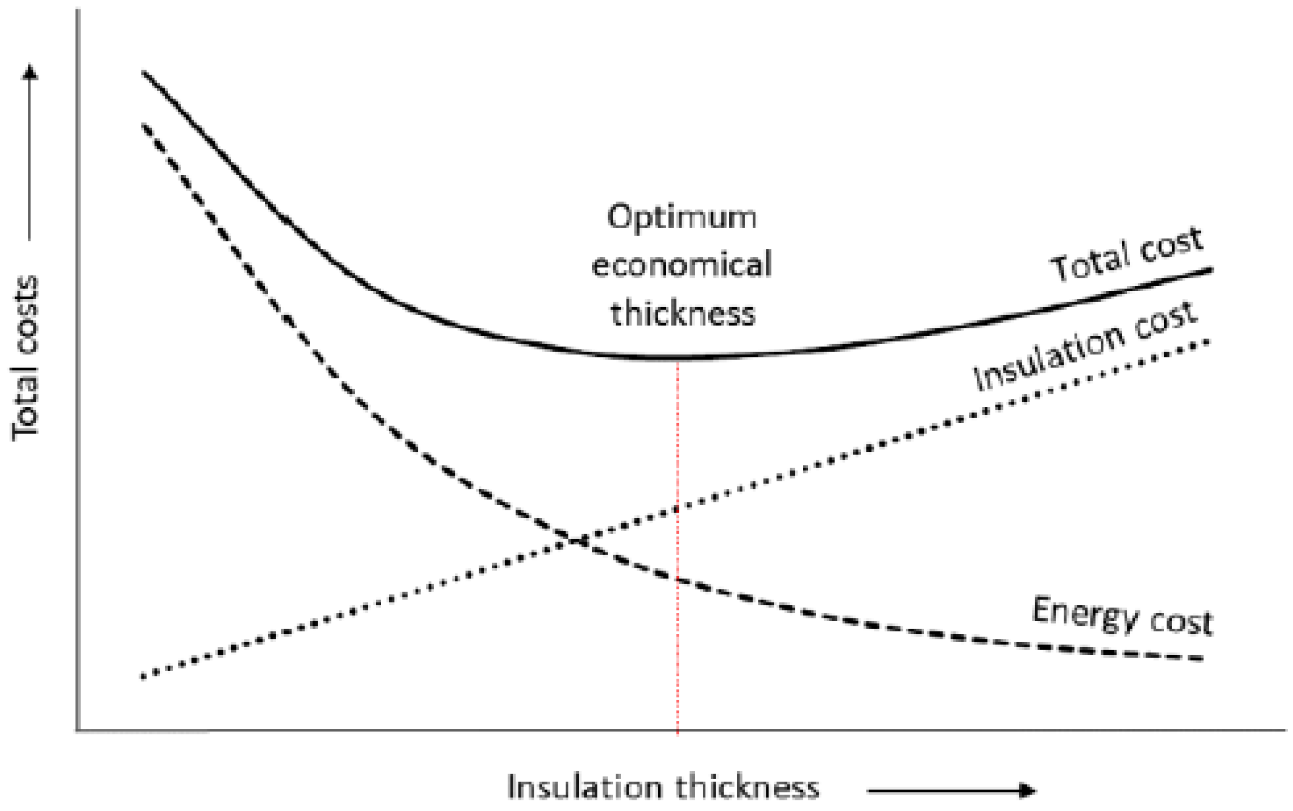
Many scientific articles emphasize the importance of passive solutions such as improving building insulation, windows’ ‘U-value’, and windows’ ‘g value’. However, the insulation level is only one parameter within total performance, typically measured by return on investment, indoor thermal comfort, and achieving NZEB benchmarks. An excessive insulation thickness increases the investment cost and may have some effect on cooling demands during the summer. Kaynakli [
7] tabulated parameters such as building type, the efficiency of installed systems, availability of energy sources and cost, etc., to estimate the optimal insulation thickness. The optimal point of insulation thickness based on investment cost and yearly energy-saving potential is shown in
Figure 1. The total cost needs to be calculated as a life cycle cost for a specified period because energy costs occur every year. Optimal insulation may be considered as one component within the cost-optimal calculation [
8], which also covers technical building systems and energy sources. In a similar context, Ibrahim et al. found the wall orientation dependency on finding the optimal insulation thickness of external walls [
9].
The optimum thermal transmittance coefficient of building facade and windows require to ensure the low investment and life cycle cost, improving building energy efficiency that complies with the national NZEB benchmark and a healthy indoor climate condition. Rosti et al. [
10] obtained the ideal insulation thickness of the external wall in eight climate zones in Iran. The results were obtained from the numerical solution under dynamic thermal conditions, which acknowledged the energy-saving potentials and payback period. Bolatturk [
11] used a life-cycle cost analysis approach, similar to Rosti et al. [
10], to find out the optimum insulation thicknesses for four climate zones in Turkey. Beyond these, D’Agostino et al. [
12] used the cost-optimal methodology to describe the optimum insulation thickness of an office building for cities of Palermo, Milan, and Cairo. In addition to life cycle cost, optimal insulation may be approached from cooling and environmental aspects as done for several cities and climate zones [
7,
13,
14,
15].
All these studies have not explicitly accounted for window properties and the window-to-wall ratio (WWR) in annual energy needs while proposing optimal insulation thickness. So far, very few studies have acknowledged the effects of windows properties and window to wall ratio while demonstrating the cost-optimal solution. Such combined effects seem substantial, as studies have shown variation in the optimal solution of wall insulation for different glazing types and areas [
15,
16,
17,
18,
19]. Thalfeldt et al. determined the cost-optimal facade solution for the Estonian climate [
18]. The results showed the promotion of energy efficiency of a building by improving the U-value of windows, low emissivity coating, and daylight considering a selection of WWRs. In a similar context, Pikas et al. proposed a fenestration design solution for an Estonian office building. This study concluded that a small window-to-wall ratio and an insulation thickness of 0.2 m were the most cost-optimal solution for the Estonian climate [
19].
In the optimum insulation analyses, many researchers have used the degree days method to estimate energy needs [
11,
13,
20]. The degree days method considers the steady-state condition, and it is related to the climate variable of air temperature only. The main drawback of the degree days method that it assumes the energy need being proportional to the difference between outdoor air and the base temperature. The base temperature requires taking into account the effect of the dynamic behavior of weather, internal and solar heat gains, and thermal mass; otherwise, it could lead to considerable errors of heating need and optimal insulation thickness solution [
21]. In the same context, Harvey [
22] found a limitation of the heating degree day (HDD) method, which could not estimate the heating demand accurately because of it accounting for daily balance point temperatures. Similarly, cooling load is poorly estimated by using the degree days approach due to ignoring the solar radiations and internal heat gains [
23]. However, degree days still may be used as a climate variable if the transient behaviors are taken into account in an energy simulation [
24,
25,
26]. Ahmed et al. [
26] applied a dynamic energy simulation for a reference office building in which heating, cooling, and lighting needs were analyzed in four climates. While economic insulation thickness was known in one climate, it was possible to calculate economic insulation with Equation (1) in other climates, enabling one to compare the buildings or energy performance requirements in different countries.
where,
is optimal thermal transmittance of the respective building for a reference climate (W/m
2K),
is the optimal thermal transmittance of building for a respective climate (W/m
2K),
is the heating degree days of building for a respective climate (°Cd),
and is the heating degree days of building for a reference climate (°Cd).
In the sequence of development, the proposed method was modified by minimizing the effect of climatic parameters [
27]. The modified method proposed a single parameter for building conductance, which was used for the adjustment of insulation thickness and window ‘U-value’ by using Equation (1) [
28]. However, the accuracy of Equation (1) has never been tested. The detailed derivation of Equation (1) is described in [
26,
27]. The derivation is based on the approximation that there is a linear dependency between the heat loss of the external wall and heating energy need. With this approximation, the minimum annual cost of the wall, depending on the insulation thickness, can be found by setting the derivative to zero, resulting in a square root dependence of heating degree days. However, it is well known that in highly insulated buildings with heat recovery, there are more complicated dependencies because of the significant contributions from internal and solar heat gains.
In this study, we derive the dependency of the optimal insulation thickness on the climate. We propose a power function instead of the square root function of Equation (1) to give more accurate climate normalization results. The accuracy of the power function was validated in four different climates. The developed method can be used for energy performance comparison of similar buildings in different climates and also for energy performance requirement comparisons.
2. Methods
This study aimed to analyze how the optimal insulation depends on the climate and to test the validity of Equation (1) to find out how degree days can be used in order to recalculate the optimal insulation for another climate. For this purpose, a procedure was used to estimate the optimal thermal insulation of the building envelope and the corresponding heating and cooling needs. Dynamic simulations were performed with the reference building to obtain the cost-optimal solution of thermal transmittance of external walls and windows. The cost-optimal solution was solved in four climates together with parametric analyses of the window to wall ratio, g-value, and energy prices, which provided versatile datasets to test the applicability of Equation (1). These findings resulted in a power function, which replaced the square root function. Therefore, the hypothesis of the study was to determine the power function, which could give more accurate climate normalization results compared to the square root function. The assessment of optimal thermal insulation of the building envelope and the corresponding heating and cooling needs was performed as follows:
- Step 1:
A reference office building was simulated with input values from the EN 16798-1:2018 standard (
Table 1) and test reference year (TRY) weather file of the corresponding climate.
- Step 2:
Two continuous variables, namely windows’ thermal transmittance and thermal resistance of external wall insulation, and three discrete variables, namely window-wall-ratio (WWR), the solar heat gain coefficient of windows (g value), and the unit cost of energy, were considered.
- Step 3:
Cost functions of window (Equation (2)) and wall insulation (Equation (3)) as well as cost-optimal Equations (Equation (6)) were constructed.
- Step 4:
Cost-optimal solution for each climate were found, including energy needs for heating and cooling, thermal transmittance of windows and external walls.
- Step 5:
Degree days were calculated with actual, variable base temperature by using Equation (7).
- Step 6:
The same steps 1–5 were followed in four climates. The reference climate could be any of these, but in this case, it was Tallinn TRY.
- Step 7:
Equation (9) was applied to obtain the power function.
Furthermore, three different WWRs (30%, 40%, and 50%), two g values of window (0.22 and 0.35), different unit costs of heating and electricity were used in parametric analyses in steps 1–7. Parametric analyses demonstrate the accuracy of the new equation.
A whole year energy simulation was conducted by using IDA Indoor Climate and Energy (IDA-ICE) building simulation tools [
29]. The Building Services Engineering division of the Royal Institute of Technology (KTH) and The Swedish Institute of Applied Mathematics have jointly developed the building simulation tools [
30], which have been further validated by EN 13791 [
31]. In this context, Travesi et al. [
32] found a good agreement between measured and simulated data while conducting an empirical model validation of different simulation tools. The simulation tools here are suitable for multi-zone complex building modeling with variable time steps and allow modeling of the dynamic heat and mass flow, energy performance, and indoor climate condition evaluation with higher accuracy.
2.1. Building Description
The reference building model was an Estonian cost-optimal office building [
33]. It was six storied massive concrete structure. The net floor area and envelop area for the single floor were 837.0 m
2 and 411.2 m
2, respectively. Besides, the total floor and envelop areas for a whole building model were 2325.5 and 4451.8 m
2, respectively. Thermal transmittance of the roof, external floor, internal floor, internal wall, and door were 0.11, 0.13, 0.24, 0.30, 1.5 W/m
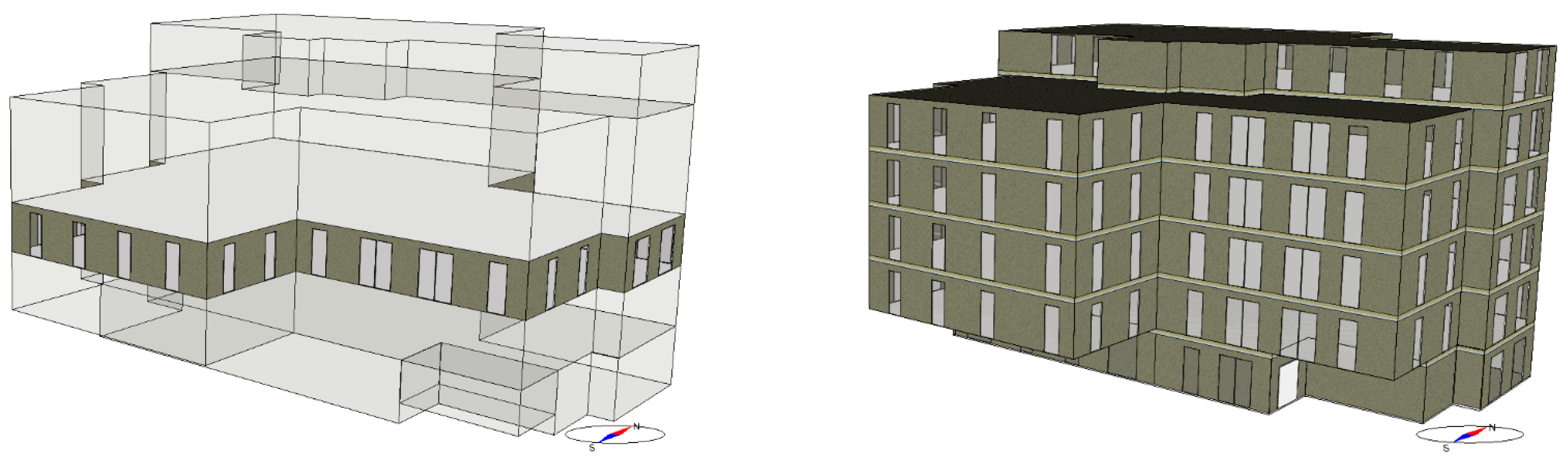
2K, respectively, which were kept the same for all climates. For the first case, the window-wall-ratio (WWR) was 30% for both the single floor and the whole building model.
The building model was north-south oriented. The solar heat gain and transmittance coefficient of the windows were 0.35 and 0.15. Air leakage rate was 1.0 L/h at the pressure difference of 50 Pa, and thermal bridges were reported as approximately 9% of total heat losses. Besides, the building model was considered as having a standard air handling unit with 80% heat recovery facility, heating coil, cooling coil, and fans. The specific fan power was considered at 1.56 kW/(m
3/s). In addition, an ideal heater and cooler with Proportional Integral (PI) control were used to keep the room temperature according to setpoints during the working hours. Also, a ventilation rate of 1.4 L/(s·m
2) was found to be sufficient to keep the indoor CO
2 level below 600 ppm. The views of a single floor and a whole building are shown in
Figure 2. Input data for energy simulation followed the EN 16798-1:2018 standard [
34,
35], as shown in
Table 1. When compared to analyses in [
36], it can be seen that ventilation and thermal comfort input data corresponded to indoor climate Category II. In addition, metabolic rate, clothing insulation were considered of 1.2 met and 0.85 ± 0.25 clo., respectively. Considering the occupant density, the ventilation rate given in
Table 1 was equivalent to 23.4 L/s per person. All input data were kept the same for all climates except the weather files. The weather file (test reference years) of Tallinn, Estonia; Brussels, Belgium; Paris, France; and Sapporo, Japan followed the American Society of Heating, Refrigerating and Air-conditioning Engineering (ASHRAE) weather files.
2.2. Continuous Variables, Cost Functions, and Cost Optimality
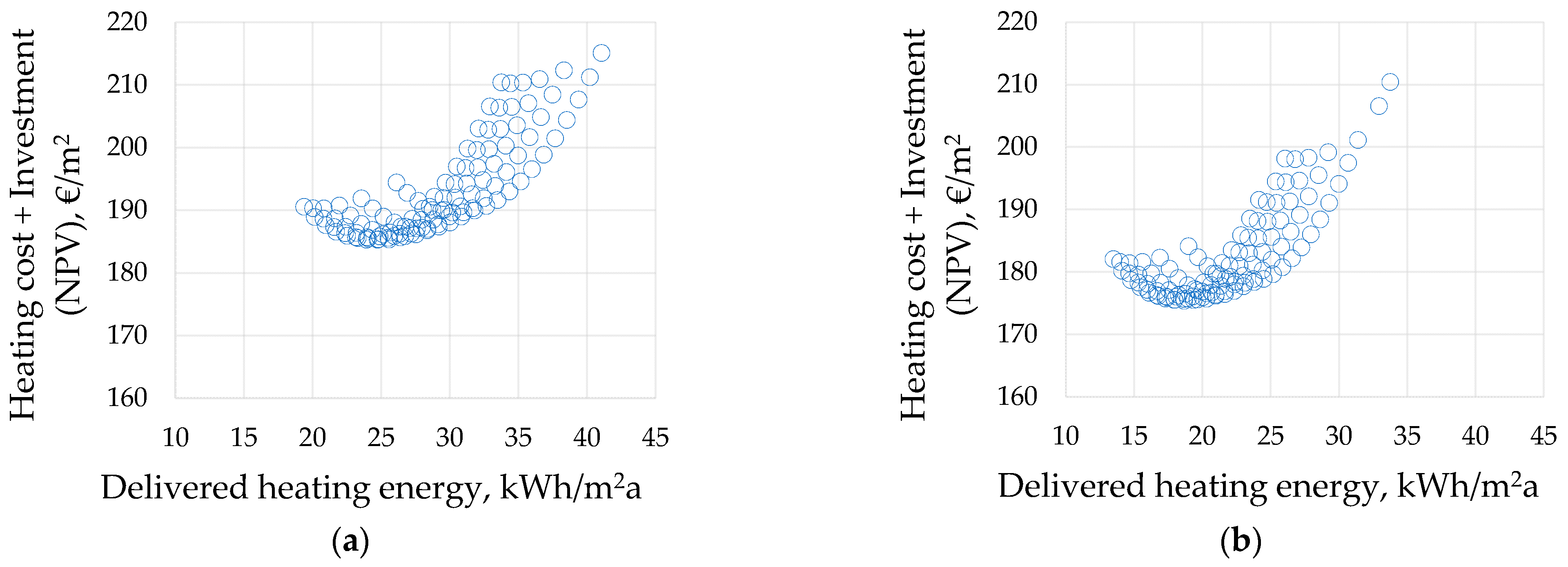
Two continuous variables, i.e., window transmittance and thermal resistance of wall insulation, were used. An extensive range of wall insulation thickness (0.05–0.40 m; step 0.05) and thermal transmittance of window (0.5–2.5 W/m
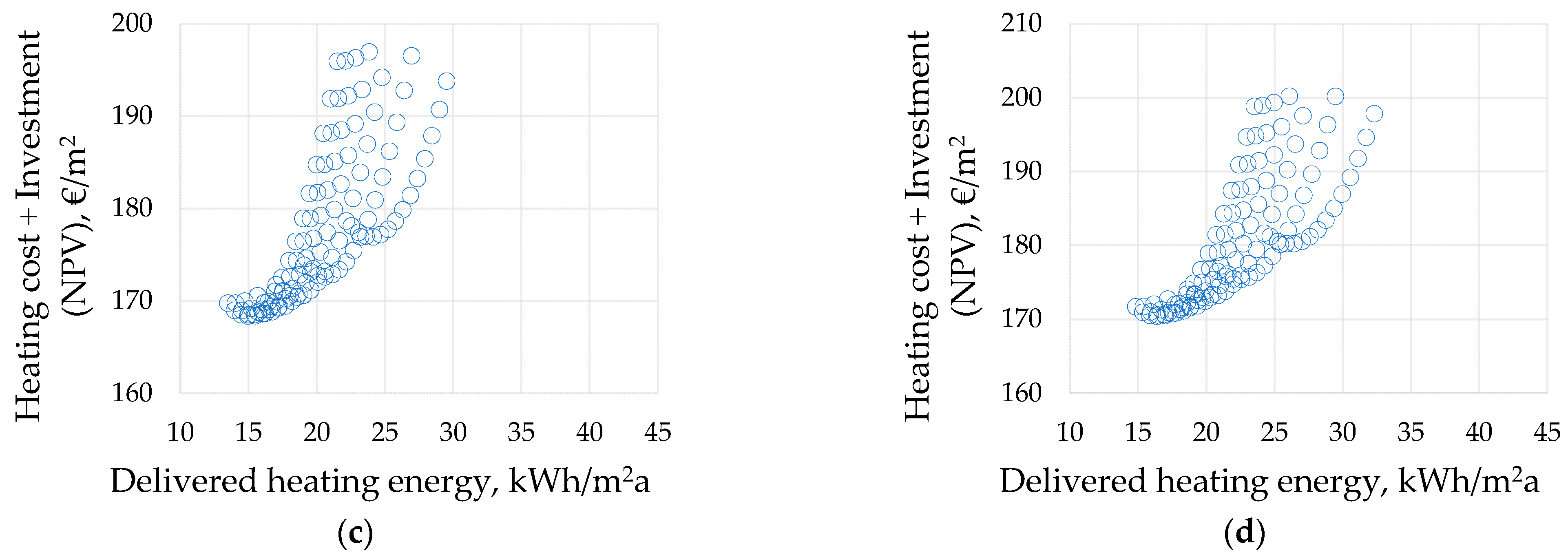
2K; step 0.1) were studied for all climates. The range became concise based on the data cloud. The boundary condition of input data of parametric simulation is shown in
Table 2. The parametric simulations were performed for a single floor model (mid-floor of the building) and a whole building model to show the effects on a different scale.
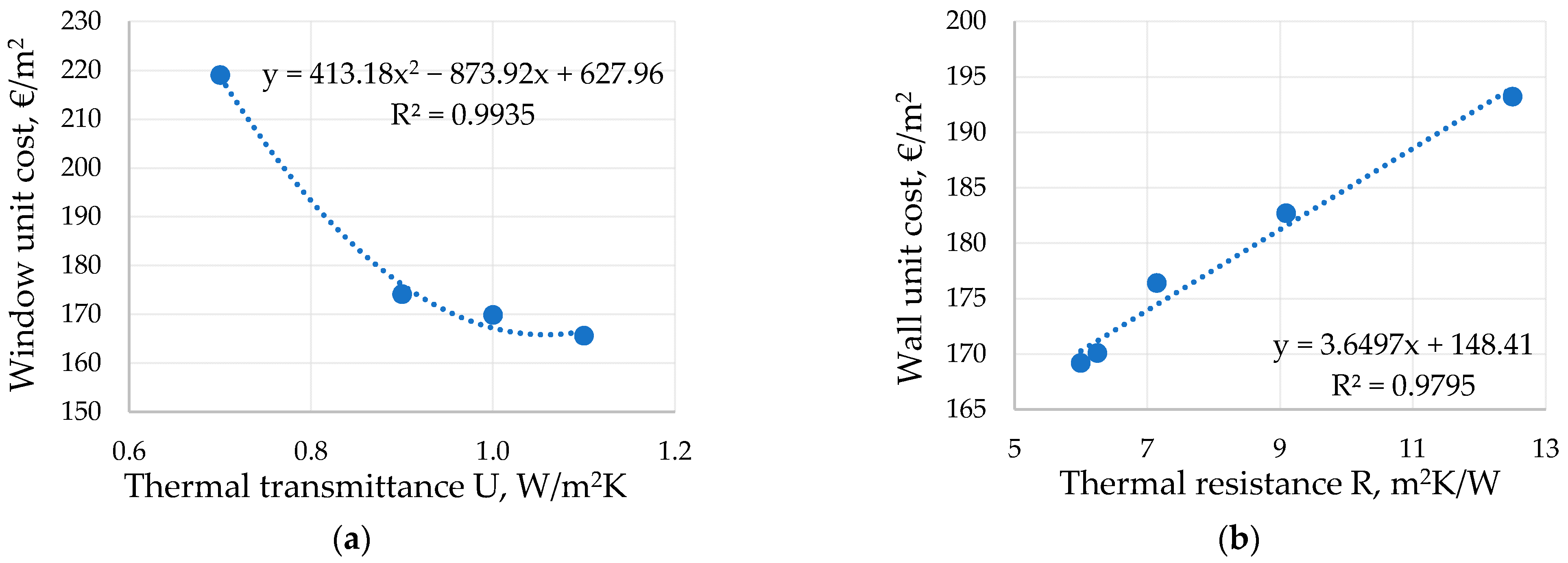
The Estonian cost functions of the window and wall insulation were used [
33]. The investment cost of the window was reported as corresponding to the thermal resistance (Equation (2)), whereas the cost function of an external wall was reported corresponding to the thermal transmittance (Equation (3)). The same cost functions were used for all climates, as shown in
Figure 3. These cost functions were based on brands and products available in Estonian markets and have been previously used for Estonian cost-optimal calculations.
where,
is the unit cost of a window (€/m
2),
is the thermal transmittance of a window (W/m
2K),
is the unit cost of a wall (€/m
2), and
is the thermal resistance of a wall (m
2K/W).
The cost-optimal equation was developed based on the investment cost of a wall, window, ground floor, roof, and the delivered energy cost, as shown in Equations (4)–(6). The unit cost of heating and electricity was assumed of 0.07 and 0.1 kWh/m
2a, respectively. Besides, the real interest and escalation rates were assumed of 2% and 1%, respectively, for 20 years.
where,
presents the value factor (−),
is the real interest rate (%),
is the escalation (%),
is the number of years,
is the total energy price considering a present value factor (€),
is the heating energy use (kWh),
is the heating energy price (€/kWh),
is the cooling energy use (
),
is the cooling energy price (€/kWh),
is the lowest cost (investment and operational cost) (€),
is the cost of total external walls (€),
is the cost of total windows (€),
is the cost of a roof (€), and
is the cost of a ground floor (€).
The heat transmission coefficient of the roof and ground floor were assumed discrete variables, and unit cost followed the same as the external wall. The optimal cost was found (Equation (6)), and corresponding window transmittance (U-value), the thermal resistance of wall insulation (R-value), energy need, and conductance were tabulated.
2.3. Sensitivity Analysis
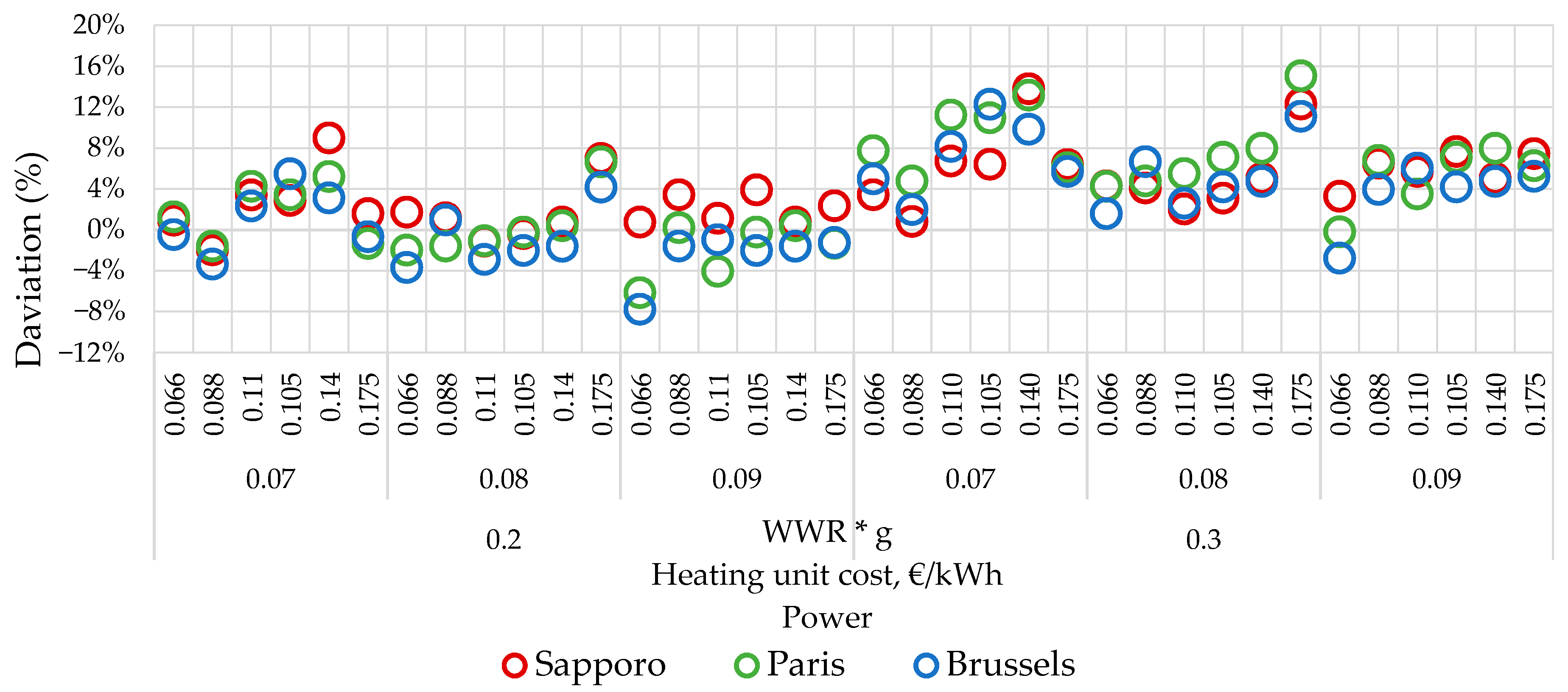
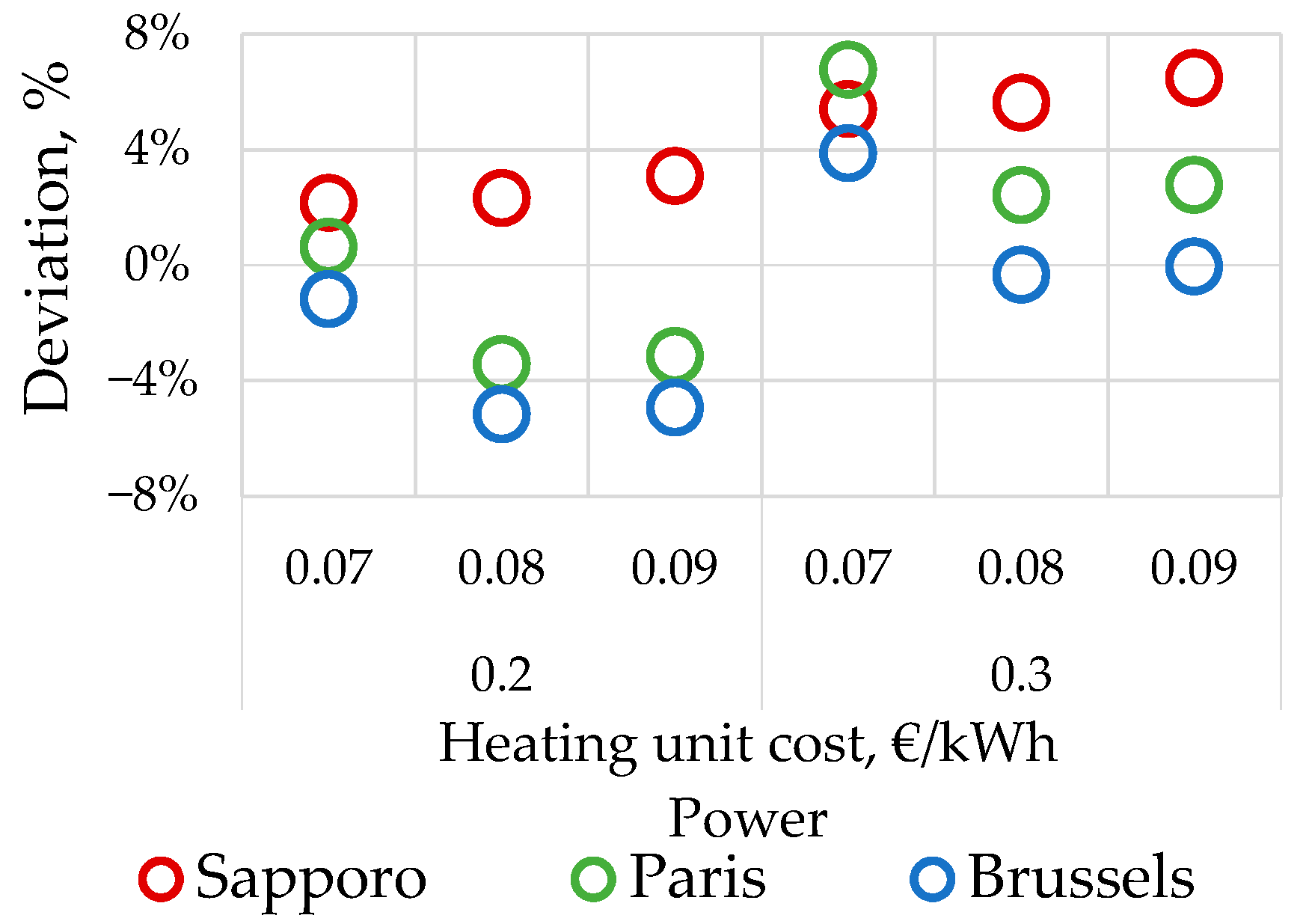
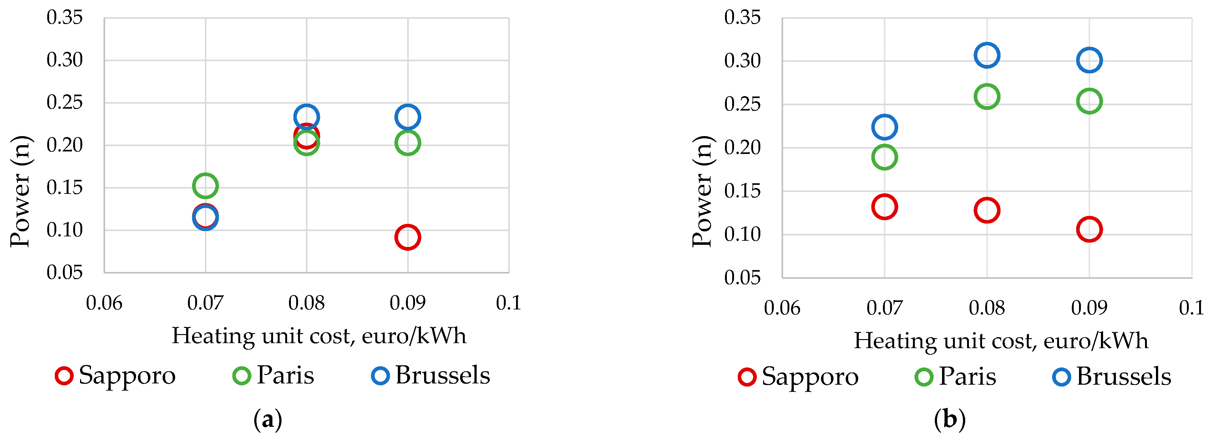
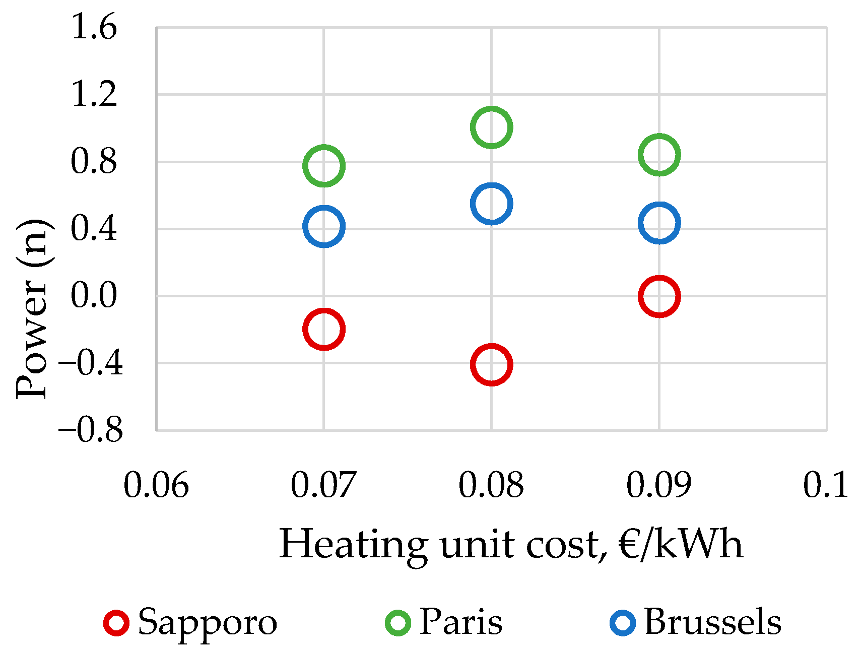
This method also tested the cases of three WWR ratios (30%, 40%, and 50%), two window’s g values (0.22 and 0.35), different unit costs of heating (0.07, 0.08, and 0.10 €/kWh), and electricity (0.1, 0.12, and 0.14 €/kWh). Six combinations of WWRs and ‘g’ values were considered, as shown in
Table 3. All these conducted tasks generated an acceptable range of power ‘n’.
4. Conclusions
This study developed a new equation for the assessment of building envelopes’ optimal insulation in different climates for office buildings. The developed method suggests determining actual degree days from simulated heating energy need and the thermal conductance of a building, avoiding in such a way the use of the base temperature. The method was tested in four climates and validated against cost-optimal solutions solved with optimization. The accuracy of the method was assessed with sensitivity analyses of key parameters such as WWRs, window g-values, costs of heating, and electricity.
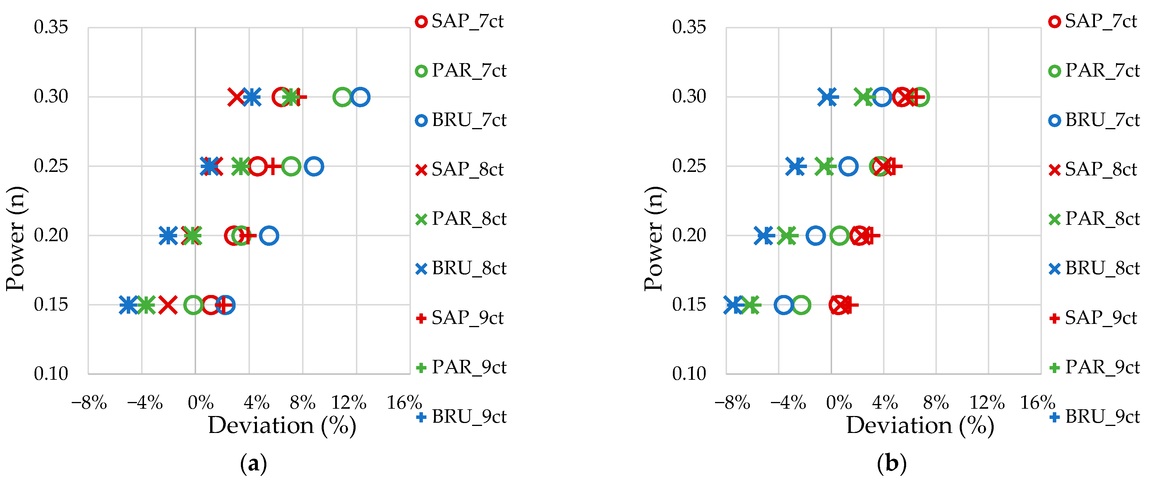
For the validation of the developed method, the cost-optimal solutions for every climate based on cost functions of external wall and windows as well as energy costs were determined, resulting in area-weighted average U-values in all four climates. The actual degree days were calculated for every climate with Equation (7). These results allowed testing of the performance of the existing square root formula (Equation (1)), showing that the climate difference effect was overestimated, i.e., calculation from the cold climate U-value would result in less insulation than cost-optimal in warmer climates. Parametric analyses revealed that the power value would provide the best possible accuracy and varied between n = 0.15 and 0.30, but n = 0.2 worked well in all cases and can be recommended as a default value.
An attempt was made to apply an optimal insulation method with heating and cooling energy in order to describe also climate differences effect on cooling energy. However, as the insulation thickness and U-value of the window have a direct effect on the heating energy but minimal effect on cooling energy, the normalization based on the total energy (heating and cooling) was not successful. Therefore, the cooling energy differences caused by climate cannot be described by insulation.
In the cost optimization, indoor air quality was not compromised because Category II ventilation rates were used in all cases. The use of the room air temperature setpoint means that operative temperature and thermal comfort can be changed when the external wall and window U-values are varied. However, the cost-optimal U-values reported in
Table 4 show high thermal insulation level, and simulated operative temperatures fall well to Category II range with used 21 °C heating setpoint. Around 99.8% of indoor temperature were in the range of 21–25.5 °C.
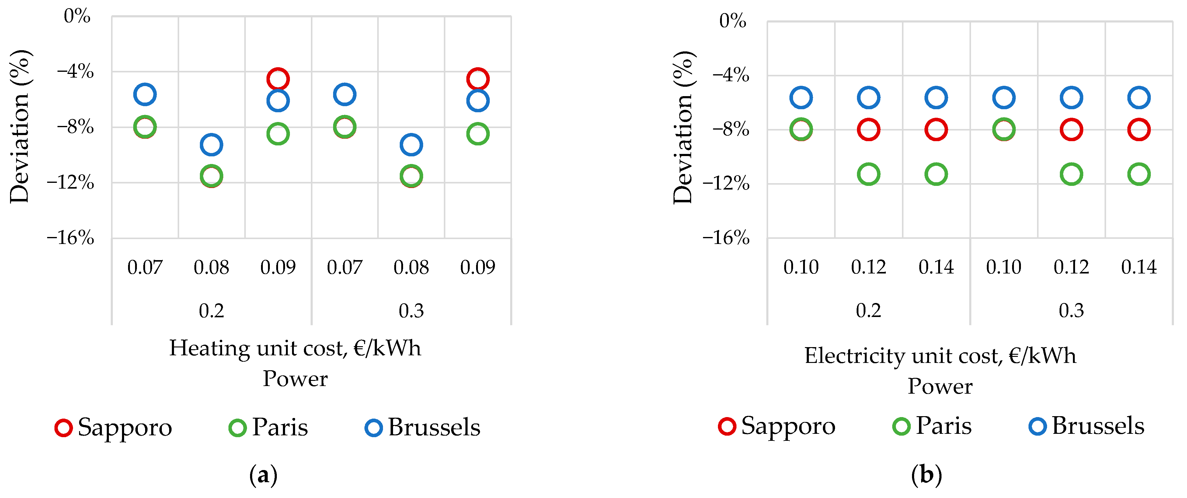
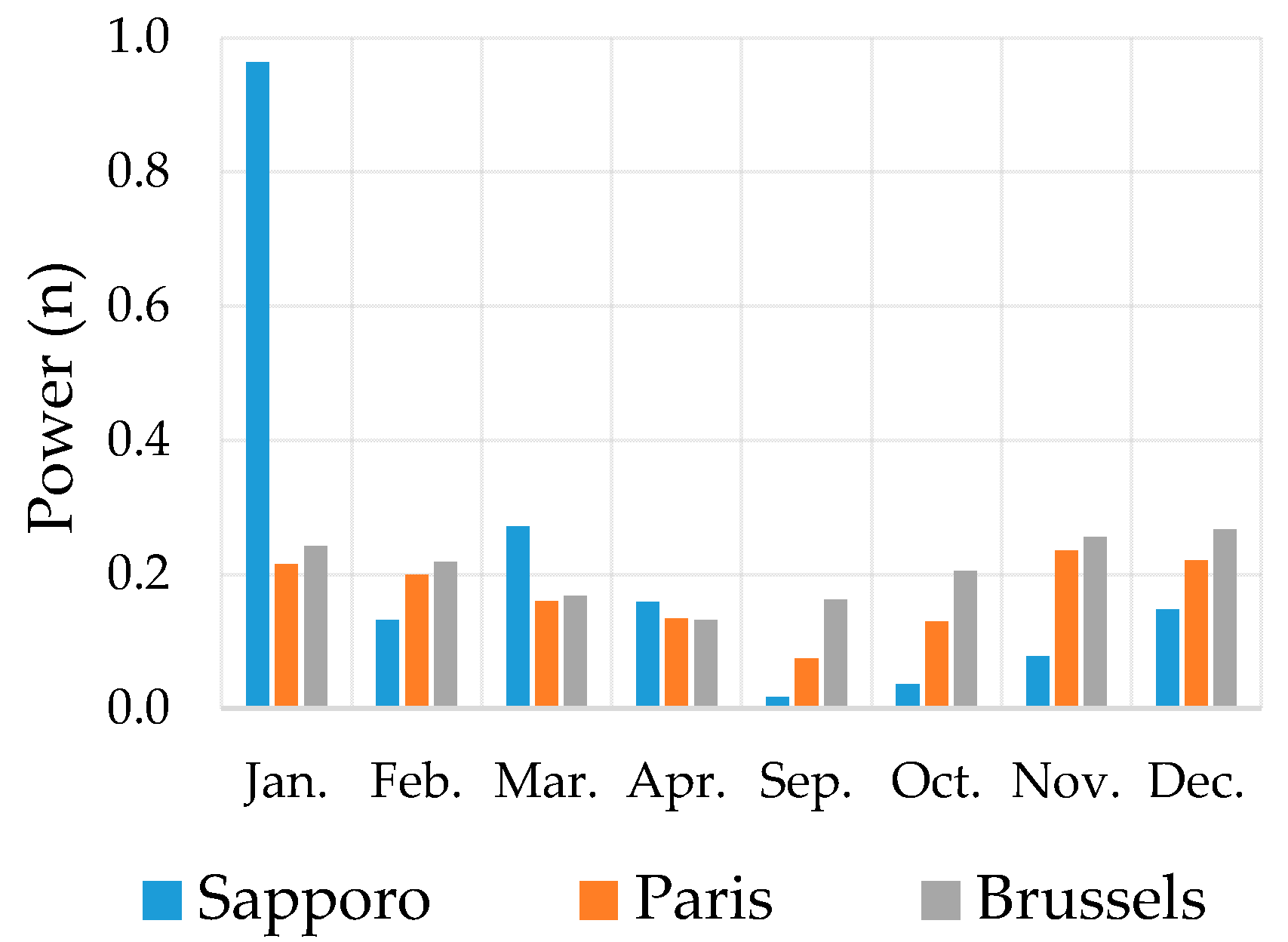
Sensitivity analyses with a broad range of energy costs, WWR, and g-values of windows revealed that the developed equation resulted in maximum 5% underestimation and maximum 7% overestimation of an average area-weighted optimal U-value of building envelope in another climate. While the method is expected to be applied mostly for insulation or annual heating energy comparisons, the actual degree days were also calculated on a monthly basis and also showed consistent performance on a monthly level.
The developed method allows objectively to compare optimal insulation of the building envelope in different climates. The method is easy to apply for energy performance comparison of similar buildings in different climates and also for energy performance requirements comparison.


