Online State-of-Charge Estimation Based on the Gas–Liquid Dynamics Model for Li(NiMnCo)O₂ Battery

Abstract

Accurately estimating the online state-of-charge (SOC) of the battery is one of the crucial issues of the battery management system. In this paper, the gas–liquid dynamics (GLD) battery model with direct temperature input is selected to model Li(NiMnCo)O₂ battery. The extended Kalman Filter (EKF) algorithm is elaborated to couple the offline model and online model to achieve the goal of quickly eliminating initial errors in the online SOC estimation. An implementation of the hybrid pulse power characterization test is performed to identify the offline parameters and determine the open-circuit voltage vs. SOC curve. Apart from the standard cycles including Constant Current cycle, Federal Urban Driving Schedule cycle, Urban Dynamometer Driving Schedule cycle and Dynamic Stress Test cycle, a combined cycle is constructed for experimental validation. Furthermore, the study of the effect of sampling time on estimation accuracy and the robustness analysis of the initial value are carried out. The results demonstrate that the proposed method realizes the accurate estimation of SOC with a maximum mean absolute error at 0.50% in five working conditions and shows strong robustness against the sparse sampling and input error.

1. Introduction

With the intensification of the energy crisis and environmental pollution, the research of electric vehicles (EVs) has become a strategic project to hasten progress toward sustainable development throughout the world [1]. Battery management system (BMS) is an important part of EVs and a core issue in the current research field of new energy vehicles. The functions of BMS include battery parameter detection, battery state estimation, online fault diagnosis, battery thermal control, etc. Among them, the real-time estimation of the state-of-charge (SOC) is one of the fundamental issues of BMS [2].

For EVs, SOC reflects the remaining capacity of the battery, which is the basis of the remaining mileage calculation. The correct estimation of SOC can not only improve the efficiency of EVs but also protect the battery and increase the battery’s service life, thereby generating economic benefits [3,4]. The charge and discharge process of the battery is a quite complicated nonlinear electrochemical reaction process [5]. As a result, different from offline SOC which is relatively easy to be obtained by discharging experiment in the laboratory, online SOC is difficult to obtain from the internal chemical characteristics of the battery and can only be estimated indirectly by some measurable parameters, such as terminal voltage, current and temperature [6].

At present, scholars have proposed a great variety of methods for accurately estimating SOC. The model-based method is one of the most commonly used approaches in practical applications [7]. The model-based SOC estimation methods are usually divided into the method based on the electrochemical model and that based on the equivalent circuit model [8,9,10]. The electrochemical model parameters have actual physical meanings and can reflect the relationship among physical quantities in electrochemical reactions inside the battery [11]. However, due to a large number of partial differential equations to solve, the on-board application of this method is difficult to realize [12]. Compared with the electrochemical model, the equivalent circuit model is widely used in battery SOC estimation for its fewer parameters and simpler mathematical expression [13]. Common SOC estimation methods based on equivalent circuit models are usually based on observer technology, including particle filter [14], sliding mode observers [15] and Kalman filtering [16]. However, the trade-off between the estimation accuracy and computational complexity for the equivalent circuit model is a troublesome problem. Furthermore, as the orders of resistance-capacitance (RC) grow, the difficulty of parameter identification and uncertainty of models are visibly increasing because one more RC will lead to one more state equation and two more uncertain parameters [7]. In addition to the above two models, Chen proposed a universal and feasible gas–liquid dynamics (GLD) battery model without significantly increasing the complexity and the amount of calculation to estimate the SOC of the battery, which is robust against different types of batteries [17]. The GLD battery model based on several gas equations and Bernoulli equation in the gas–liquid system reflects the electron transference, terminal voltage lag, Li+ diffuseness and equilibrium, ohmic effect, etc., in lithium-ion batteries (LIBs). Neither complicated optimization algorithms nor matrix operations are applied to ensure the real-time performance of SOC online estimation. However, the above GLD model only considers offline parameter identification and does not conduct a more in-depth study on the online parameter identification of the model.

As the accuracy of using offline identification parameters to estimate SOC will decrease with working time increasing and working condition varying [6]. Some online parameter identification methods are proposed to eliminate errors caused by parameter changes. Wang et al. proposed a recursive least squares (RLS) approach for online parameter identification [18]. This method corrects the previously estimated value by the recursive algorithm after the new observation result is obtained until the new estimated result reaches the set accuracy. Khare et al. [19] improved RLS method and proposed a forgetting factor recursive least-square (FFRLS) method for parameter identification, which could avoid the occurrence of RLS “Data saturation” phenomenon. Apart from the common RLS and its derivatives, Kalman filter (KF) and its derivatives have also become popular techniques for addressing the issue of online state or parameter estimation for both linear and nonlinear systems. The extended Kalman Filter (EKF) was first applied to state and parameter identification in BMS and proven to be a reliable approach for online estimation by Pet [20,21,22]. Based on the first-order RC circuit model, an EKF is introduced for battery parameters online identification only using current and voltage by Wang et al. [23]. Similarly, Pei et al. [24] used the dual extended Kalman filter (DEKF) based on an equivalent circuit to estimate the parameters only by the load current and terminal voltage instead of temperature and ageing. Xiong et al. [25] proposed an adaptive extended Kalman filter (AEKF) to overcome the drawback that traditional KF is too dependent on the good estimation of the process and measurement noise matrix Q and R. This method avoids that uncertainty of the initial noise information results in the degrading the estimation performance but it lacks analysis for cell parameter variances under different temperatures. To compensate for this drawback, Feng et al. [26] proposed an online parameters identification method by exploiting KF and adapted to concurrently estimate both state and parameters, thereby realizing online simultaneous update of states and parameters at various ambient temperatures. To effectively eliminate the deviation caused by first-order approximation of Taylor series expansion in EKF, an unscented Kalman filter (UKF) is proposed by Xing et al. [27] to cope with uncertainties of the working condition and battery model inherent inaccuracy. Additionally, Genetic algorithm (GA) can also be applied for online parameter identification of batteries [28].

For the experimental verification of battery SOC estimation, normally a single working condition such as Constant Current (CC), Dynamic Stress Test (DST), Federal Urban Driving Schedule (FUDS) and Urban Dynamometer Driving Schedule (UDDS) is used in most of the above-mentioned studies. However, many operating conditions in the actual operation of vehicles are often changing. For instance, different drivers have different driving styles [29]. People who are accustomed to driving in an aggressive and almost bullying manner tend to speed and weave in and out of traffic, making the EVs’ battery often discharge at a high C-rate. On the contrary, defensive drives prefer to follow and obey posted signs and speed limits to avoid rapid acceleration and deceleration, making the battery discharge and charge C-rate more stable. Apart from that, people often drive on different roads and switch driving scenes, such as highways, suburbs and cities. The above facts mean that there may be a variety of working conditions in one discharge cycle corresponding to the battery of an electric vehicle in real situations. To address this issue, Du et al. [30] collected the data from the actual driving condition to verify their SOC estimation. There is little research on the combination of the driving cycles and to simulate the actual driving condition, most of the studies refer to the standard single cycle (DST, UDDS, etc.) [31,32,33], perhaps because different working conditions are already included in a single cycle, such as DST cycle which uses a 360 s sequence of power steps with seven discrete power levels to represent different driving conditions. Despite this, the combination of the different cycles could be a good complement to simulating the real driving condition more realistically. Additionally, the sampling interval is also crucial in the SOC estimation process, especially for the coulomb counting approach [34]. To make the SOC estimation more accurate, it is necessary to use a higher sampling frequency for the Coulomb counting method to obtain more accurate current information [34]. For the studies on online parameters identification and estimation of SOC, many methods combined with RC model use Coulomb counting as the part of the state equation [35,36,37]. Therefore, it is difficult to implement sparse sampling for these methods. The sampling frequency in the above-mentioned research is often 1–10 HZ, which lacks exploration of algorithm performance under sparse sampling conditions. High sampling frequency can make the estimation more accurate, but the compensation for this improvement is that the cost of hardware is also greatly increased due to the demand for extra storage space and massive computing power [38]. Therefore, it is important to ensure the accurate estimation of SOC under the condition of sparse sampling, that is, increasing the sampling period to reduce costs and thus achieve practical applications.

1.1. Contribution of This Paper

In this article, from the perspective of the multiscenario, a SOC estimation method is proposed to eliminate initial errors rapidly and achieve high-precision SOC estimation under a wide sampling period and a combined condition.

First of all, the result of the offline model is transformed into the input of the online model, so the offline model and online model are coupled and the estimation error is transformed into the input error, which could achieve the goal of quickly eliminating initial errors.

Moreover, to more realistically simulate the actual charge and discharge process of electric vehicle batteries, a combined scenario including Constant Current (CC) cycle, Federal Urban Driving Schedule (FUDS) cycle, Urban Dynamometer Driving Schedule cycle (UDDS) and Dynamic Stress Test (DST) cycle is constructed. The proposed algorithm realizes the accurate estimation of SOC in a single cycle coupled with multiple operating conditions.

Additionally, a systematic study on the effect of sampling time and initial error on estimation accuracy is done in this article. The high precise estimation is still achieved under the sparse sampling and large initial error through this algorithm.

1.2. Organization of This Paper

The structure of this paper is organized as follows: In Section 2, the GLD battery model is introduced and based on that, we present offline and online parameter identification methods and they are combined to estimate the battery SOC. The experiment details including the construction of combined load profiles are presented in Section 3. Then, results and discussion of the proposed approach are demonstrated in Section 4. Section 5 summarizes the conclusions in this work.

2. Identification of Battery Model Parameters

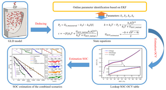
2.1. Battery Modelling

This paper uses the GLD battery model derived from a series of Gas Equation and Bernoulli Equation in the equivalent gas–liquid system [17]. Partly different from GLD battery model, the temperature is introduced to be a direct input.

The inflation and deflation process of the gas–liquid dynamics model can be equivalent to the corresponding charge and discharge process of the battery. The schematic of the GLD model is shown in Figure 1a.

Taking the discharge process of the battery as an example, at time $t_1$, it can be assumed that the GLD battery model is in a steady state, and at this time the gas pressure, the amount of substance of gas, and the amount of gas dissolved in liquid are$P_1$, $n_1$ and $n_{j1}$, respectively; The amount of gas substance dissolved in a liquid can be calculated according to the modified ideal gas law.

$$n_{j1}=\frac{P_1{\phi }_m{V}_w}{RT+b_m{P}_1}$$

(1)

where $T$ represents thermodynamic temperature; ${\phi }_m$ and $b_m$ are effective clearance and Van der Wal volume of gas molecules, respectively; $R$ is the thermodynamic constant ($R=8.314J/mol·K$).

The valve of the container is opened for a while $\mathsf{∆}t$ so that the gas in the container is released outwards (Figure 1b). During this deflation process, the flow velocity, the resistance coefficient of gas flow, and the pressure of the external nozzle are $v$, $\mu$, and $P_0$, respectively. The valve is closed at $t_2=\mathsf{∆}t+t_1$, when the gas pressure is $P_2$ and the amount of substance of gas is $n_2$; the ideal gas state equation and Bernoulli equation of gas flow during gas exhausting can be written as:

$$P_{2}V=n_{2}RT$$

(2)

$$P_2=P_0+\frac{1}{2}\mu v+\frac{1}{2}\rho \mu v^2$$

(3)

After a long enough time until $t_3$, the GLD battery model reaches a steady state again. At this time, the gas pressure in the container, the amount of substance of gas and the amount of substance of gas dissolved in the liquid are $P_3$, $n_3$ and $n_{j3}$, respectively; the ideal gas state equation and solubility equation of gas after rebalancing can be written as:

$$P_{3}V=n_{3}RT$$

(4)

$$n_{j3}=\frac{P_3{\phi }_m{V}_w}{RT+b_m{P}_3}$$

(5)

At the moment when the valve is closed, the amount of gaseous substance in the vessel is $n_2$; After closing the valve, the amount of gas substance of gas precipitated from the liquid is $n_{j1}-n_{j3}$; Therefore, the relationship among the amount of substance can be given by:

$$n_3=n_2+\left(n_{j1}-n_{j3}\right)$$

(6)

The Equations (1)–(6) are introduced to Equation (7)

$$P_3-P_2=\frac{R^2{T}^2{\phi }_m{V}_w}{V{b}_m^2}\times (\frac{1}{\frac{RT}{b_m}+P_3}-\frac{1}{\frac{RT}{b_m}+P_1})$$

(7)

The Equation (7) could be simplified to the following two Equations:

$$P_3-P_2=k_1{k}_2^2{T}^2\times (\frac{1}{k_{2}T+P_3}-\frac{1}{k_{2}T+P_1})$$

(8)

$$k_1=\frac{{\varphi }_m{V}_W}{V}, k_2=\frac{R}{b_m}$$

(9)

Because all the parameters have physical meanings, $k_{2}T+P_3>0$ and $k_{2}T+P_1>0.$ Equation (8) can also be written as:

$$P_3^2+P_3(k_{2}T-P_2+\frac{k_1{k}_2^2{T}^2}{k_{2}T+P_1})-(P_2{k}_{2}T+\frac{P_1{k}_1{k}_2^2{T}^2}{k_{2}T+P_1})=0$$

(10)

Assuming $a=1,b=(k_2-P_2+\frac{k_1}{k_2+P_1}),c=-(\frac{k_1{P}_1}{k_2+P_1}+P_2{k}_2)$ and $ac<0,b^2-4ac>0$, according to the Veda theorem, the equation has only one positive real root, which is given by:

$$P_3=\frac{\sqrt{b^2-4c}-b}{2}$$

(11)

The above derivation takes the process of opening the valve to release gas as an example. The derivation result of opening the valve to pump gas from the outside into the vessel is consistent with the above result.

During the air inflation process, the Bernoulli equation for pumping gas into the vessel:

$$P_2=P_0-\left(\frac{1}{2}\mu \rho v+\frac{1}{2}\rho v^2\right)$$

(12)

Therefore, the Bernoulli equation of the inflation process and the deflation process can be unified into the following formula:

$$P_2=P_0-\frac{1}{2}\mu v-\frac{1}{2}\rho \mu \left|v\right|v$$

(13)

where $v>0$ when charging, $v<0$ when discharging.

Simplifying the derived gas–liquid dynamic battery model:

$$k_3=\frac{1}{2}\mu ,k_4=\frac{1}{2}\rho \mu$$

(14)

Therefore, according to the correspondence of parameters between the GLD model and battery (

Table 1. Correspondence of parameters between the GLD model and battery.

GLD Battery Model Parameters	Actual Battery Parameters
Pressure of gas at the nozzle $P_0$	Terminal voltage $U_{0\_\mathrm{measured}}$
Gas flow velocity $v$	Electron flow $I$
Pressure of gas $P_1$ before opening the valve	Initial open-circuit voltage $U_{OCV\_\mathrm{initial}}$
Pressure of gas $P_3$ after rebalance	Estimated open-circuit voltage $U_{OCV\_\mathrm{estimated}}$
Temperature in cans $T$	Temperature of the battery $T$

), the final GLD open-circuit voltage battery model is derived:

$$P_2=U_{0\_\mathrm{measured}}-k_{3}I-k_{4}I\left|I\right|,\mathrm{charge}:I>0,\mathrm{discharge}:I<0$$

(15)

$$\begin{gathered} U_{OC{V}_{\mathrm{estimated}}}=\frac{-b+\sqrt{b^2-4c}}{2} \\ b=k_{2}T-P_2+\frac{k_1{k}_2^2{T}^2}{k_{2}T+U_{OCV\_\mathrm{initial}}} \\ c=-(P_2{k}_{2}T+\frac{U_{OCV\_\mathrm{initial}}{k}_1{k}_2^2{T}^2}{k_{2}T+U_{OCV\_\mathrm{initial}}}) \end{gathered}$$

(16)

2.2. Offline Parameters Identification

To use the GLD model to estimate the open-circuit voltage of the battery, it is important to identify the corresponding parameters $k_1,k_2,k_3,k_4$. An offline identification method using the optimizing objective function based on GA is introduced in Reference [17]. In this article, the same method is applied to determine the first series of offline parameters, noted as parameters_offline. When the battery works under different scenarios including UDDS, DST, FUDS, CC and combined driving cycle, this set of offline parameters remains unchanged.

2.3. Online Parameters Identification by Extended Kalman Filter (EKF)

The battery model parameters are not constant but are related to the battery’s temperature, SOC, age, etc. As a result, the model parameters identified offline will cause unavoidable calculation errors during BMS working process and may even increase the error of the offline parameter model as the working time increases [6]. Moreover, offline parameters identification lack generalization ability, which means that the parameters identified under certain working conditions may not be applicable for other working conditions and lead to inherent error [23]. The advantage of the online parameter identification method is that it could simultaneously update the model parameters as the parameters change during the battery operation, thereby eliminating the parameter’s deviation [26]. However, when the initial input of the online model is incorrect, in addition to identifying online parameters, it is also necessary to eliminate the interference of initial errors. It is difficult for an online model to obtain good estimation performance quickly in the initial stage and this is likely to lead to an increase in the cumulative error of the estimation and eventually divergence of the result. The offline parameters could compensate for this disadvantage by the revision of the input due to its strong anti-interference ability. Therefore, the solution in this article is to refer to estimated OCV obtained from the offline model as the input of online estimation model, which makes the estimation error transform into input error and takes advantage of the strong anti-interference ability of the offline model to quickly eliminate the initial error.

The proposed parameter identification method is based on the EKF theorem and the derivation process is shown as follows.

Equations (15) and (16) can be written as the following functional expression:

$$U_{OCV\_\mathrm{estimated}}=f\left(k_1,k_2,k_3,k_4,I,U_{OCV\_\mathrm{initial}},U_{0\_\mathrm{measured}},T\right)$$

(17)

Replacing the parameters for the gas–liquid model with the parameters for the GLD battery model, Equation (8) could be transformed as:

$$U_{OCV\_estimated}-P_2=k_1{k}_2^2{T}^2\times (\frac{1}{k_{2}T+U_{OCV\_\mathrm{estimated}}}-\frac{1}{k_{2}T+,U_{OCV\_\mathrm{initial}}})$$

(18)

Then, based on Equation (18), $P_2$ can be expressed by:

$$P_2=U_{OCV\_\mathrm{estimated}}-k_1{k}_2^2{T}^2\times (\frac{1}{k_{2}T+U_{OCV\_\mathrm{estimated}}}-\frac{1}{k_{2}T+,U_{OCV\_\mathrm{initial}}})$$

(19)

Substituting $P_2$ in Equation (15) by Equation (19), the terminal voltage could be expressed by $k_1,k_2,k_3,k_4,I,U_{OCV\_\mathrm{estimated}},,U_{OCV\_\mathrm{initial}},T$:

$$U_{0\_\mathrm{estimated}}=U_{OCV\_\mathrm{estimated}}-k_1{k}_2^2{T}^2(\frac{1}{k_{2}T+U_{OCV\_\mathrm{estimated}}}-\frac{1}{k_{2}T+,U_{OCV\_\mathrm{initial}}})+k_{3}I+k_{4}I\left|I\right|$$

(20)

For the convenience of expression, Equation (20) could also be expressed as:

$$U_{0\_estimated}=f\left(k_1,k_2,k_3,k_4,I,U_{OC{V}_{\_\mathrm{estimated}}},U_{OCV{\_}_{\mathrm{initial}}},T\right)$$

(21)

Equations (17) and (21) require 7 input parameters, respectively. The meaning of each parameter is as follows:

For Equation (17),$k_1,k_2,k_3,k_4$ are identified by offline method and remain unchanged during the whole working period; which can be noted as $k_{1\_\mathrm{offline}},k_{2\_\mathrm{offline}},k_{3\_\mathrm{offline}},k_{4\_\mathrm{offline}}$, $I$ represents the battery electron flow; $U_{0\_measured}, T,U_{OCV\_initial},$ are battery terminal voltage and ambient temperature measured by corresponding sensors and initial open-circuit voltage, respectively; $U_{OCV\_estimated}$ represents the estimated current OCV. For Equation (21), $k_1,k_2,k_3,k_4$ are online identified parameters and change in real-time during the whole working period; which can be noted as $k_{1\_\mathrm{online}},k_{2\_\mathrm{online}},k_{3\_\mathrm{online}},k_{4\_\mathrm{online}}$. $I$ represents the battery electron flow; $U_{OCV\_\mathrm{initial}},T,U_{ocv\_\mathrm{estimated}}$ are initial open-circuit voltage, ambient temperature and estimated current open-circuit voltage by Equation (17), respectively, where the $U_{ocv\_\mathrm{estimated}}$ is an output of Equation (17) with systematic error caused by the offline GLD model error.

In order to use EKF to update the parameters in real-time, the state vector is set as:

$$Par{a}_k={\left[k_{1\_\mathrm{online}\_k},k_{2\_\mathrm{online}\_k},k_{3\_\mathrm{online}\_k},k_{4\_\mathrm{online}\_k}\right]}^T$$

(22)

It can be assumed that since the sampling time of the system is several seconds, which is quite short, the system parameters will only change slightly between two sampling intervals $t_k,t_{k+1}$. Therefore, the discrete state transition matrix for parameters is given by:

$$Par{a}_{k+1}=Par{a}_k+w_k$$

(23)

where $w_k$ represents the process noise and its covariance is Q, noted as $w_k\in N\left(0,Q\right)$.

The discrete state observation matrix is expressed as:

$$U_{0\_\mathrm{measured}\_k+1}=H·Par{a}_{k+1}+u_{k+1}$$

(24)

where the state observation matrix $H$ is partial derivative matrix of $k_1,k_2,k_3,k_4$ in Equation (20). $H=\left[\begin{array}{cc}\begin{array}{cc}\frac{\partial U_{0\_\mathrm{estimated}}}{k_{1\_\mathrm{online}}}& \frac{\partial U_{0\_\mathrm{estimated}}}{k_{2\_\mathrm{online}}}\end{array}& \begin{array}{cc}\frac{\partial U_{0\_\mathrm{estimated}}}{k_{3\_\mathrm{online}}}& \frac{\partial U_{0\_\mathrm{estimated}}}{k_{4\_\mathrm{online}}}\end{array}\end{array}\right]$. $u_{k+1}$ is the measurement noise which represents the deviation caused by measurement noise and the observation deviation of the observation matrix itself, and its covariance is R, noted as $u_{k+1}\in N\left(0,\mathrm{R}\right)$.

Assuming that $par{a}_k,par{a}_{k+1}$ represent the true value matrixes of the parameter at time $t_k,t_{k+1}$, and $\widetilde{par{a}_{k+1}},\overline{par{a}_{k+1}}$ represent a prior state estimate and a posteriori state estimate, respectively.

The prior state estimate can be obtained from the state prediction equation:

$$\widetilde{par{a}_{k+1}}=\overline{par{a}_k}$$

(25)

The posteriori state estimate can be obtained from the state update equation:

$$\overline{par{a}_{k+1}}=\widetilde{par{a}_{k+1}}+K\left(U_{0\_\mathrm{measured}\_k+1}-H·\widetilde{par{a}_{k+1}}\right)$$

(26)

where $H·\widetilde{par{a}_{k+1}}=U_{0\_\mathrm{estimated}\_k+1}$; K is a Kalman gain matrix.

Therefore Equation (26) could be written as:

$$\overline{par{a}_{k+1}}=\widetilde{par{a}_{k+1}}+K\left(U_{0\_\mathrm{measured}\_k+1}-U_{0\_\mathrm{estimated}\_k+1}\right)$$

(27)

To derive Kalman gain matrix, one can note:

$$\widetilde{e_{k+1}}=par{a}_{k+1}-\widetilde{par{a}_{k+1}}$$

(28)

$$\overline{e_{k+1}}=par{a}_{k+1}-\overline{par{a}_{k+1}}$$

(29)

$$\widetilde{P_{k+1}}=E\left[\widetilde{e_{k+1}},{\widetilde{e_{k+1}}}^T\right]$$

(30)

$$\overline{P_{k+1}}=E\left[\overline{e_{k+1}},{\overline{e_{k+1}}}^T\right]$$

(31)

where $\widetilde{e_{k+1}}$ represents prior state estimate error; $\overline{e_{k+1}}$ represents posteriori state estimate error; $\widetilde{P_{k+1}}$ is the covariance between the true value and the predicted value;$\overline{P_{k+1}}$ is the covariance between the true value and the best estimation.

Combining Equations (24) and (26) to eliminate $U_{0\_\mathrm{measured}\_k+1}$:

$$\overline{par{a}_{k+1}}=\widetilde{par{a}_{k+1}}+K\left(H·Par{a}_{k+1}+u_{k+1}-H·\widetilde{par{a}_{k+1}}\right)$$

(32)

Transformation of Equation (28):

$$\overline{par{a}_{k+1}}-Par{a}_{k+1}=\widetilde{par{a}_{k+1}}-Par{a}_{k+1}+KH\left(Par{a}_{k+1}-\widetilde{par{a}_{k+1}}\right)+K{u}_{k+1}$$

(33)

Replacing $\overline{par{a}_{k+1}}-Par{a}_{k+1}$ and $\widetilde{par{a}_{k+1}}-Par{a}_{k+1}$ in Equation (33) by Equations (28) and (29):

$$\overline{e_{k+1}}=\left(1-KH\right)\widetilde{e_{k+1}}- K{u}_{k+1}$$

(34)

Therefore, the estimated error variance matrix can be known from Equation (31):

$$\overline{P_{k+1}}=\left(1-KH\right)\widetilde{P_{k+1}}{\left(1-KH\right)}^T- KR{K}^T$$

(35)

The estimation principle of Kalman filter is to minimize the covariance $P$ of the optimal state estimation and make it closer and closer to the true value. Therefore, its objective function is:

$$J={\displaystyle \sum }_{min}\overline{P_{k+1}}$$

(36)

Calculating the partial derivative of the Kalman gain matrix K in Equation (35):

$$\frac{\partial \overline{P_{k+1}}}{\partial K}=-2\widetilde{P_{k+1}}{H}^T+2K\left(H\widetilde{P_{k+1}}{H}^T+R\right)=0$$

(37)

Therefore, Kalman gain matrix K could be expressed as:

$$K=\widetilde{P_{k+1}}{H}^T{\left(H\widetilde{P_{k+1}}{H}^T+R\right)}^{-1}$$

(38)

Replacing R in Equation (35) by Equation (38):

$$\overline{P_{k+1}}=\left(1-KH\right)\widetilde{P_{k+1}}$$

(39)

Combing Equations (23), (25) and (28) to eliminate $\widetilde{par{a}_{k+1}}$,$par{a}_{k+1}$:

$$\widetilde{e_{k+1}}=par{a}_{k+1}-\widetilde{par{a}_{k+1}}=Par{a}_k+w_k-\overline{par{a}_k}=\overline{e_k}+w_k$$

(40)

According to Equation (30):

$$\widetilde{P_{k+1}}=E\left[\widetilde{e_{k+1}},{\widetilde{e_{k+1}}}^T\right]=E\left[\left(\overline{e_k}+w_k\right),{\left(\overline{e_k}+w_k\right)}^T\right]$$

(41)

$$\widetilde{P_{k+1}}=\overline{P_k}+Q$$

(42)

Therefore, all the unknowns are determined in Equation (26) and the online parameter identification at one step is finished.

2.4. Combination of Offline Parameters and Online Parameters for SOC Estimation

The joint algorithm can be summarized as follows:

(1)

Initialization

The covariance between the true value and the best estimate at the initial time:

$$\overline{P\left(0\right)}=diag\left(\left[1,1,1,1\right]\right)$$

(43)

All parameters in physical equations have actual physical meaning, so all parameters are non-negative including $k_1,k_2,k_3,k_4$.and they cannot be initialized to be zero. Therefore, the initial parameters for online identification are set to close to zero which is (0.001,0.001,0.001,0.001). Additionally, step k is set as 1.

(2)

Assignment

The current electron flow, terminal voltage and ambient temperature could be obtained by corresponding sensors at step k, noted as, $U, I,T$. These three variables are assigned to corresponding variables $U_0\left(k\right)$ $I\left(k\right)$ and $T\left(k\right)$, respectively.

$$U_0\left(k\right)=U,I\left(k\right)=I,T\left(k\right)=T,U_{OCV{\_}_{\mathrm{initial}}}\left(1\right)=U_0\left(1\right)$$

(44)

(3)

Calculation 1

According to Equation (17) and offline parameters in Section 4.1, the estimated open-circuit voltage $U_{OCV\_estimated\_k}$:

$$U_{OCV\_\mathrm{estimated}}\left(k\right)=f\left(U_{OC{V}_{\_\mathrm{initial}}}\left(k\right),U_0\left(k\right),k_{1\_\mathrm{offline}},k_{2\_\mathrm{offline}},k_{3\_\mathrm{offline}},k_{4\_\mathrm{offline}},I\left(k\right),T\left(k\right)\right)$$

(45)

Then, $U_{OCV\_\mathrm{estimated}}\left(k\right)$ is set as one of the inputs to obtain estimated terminal voltage $U_{0\_\mathrm{estimated}}\left(k\right)$:

$$U_{0\_\mathrm{estimated}}\left(k\right)=f\left(U_{OC{V}_{\_\mathrm{estimated}}}\left(k\right),\overline{para\left(k-1\right)},I\left(k\right),T\left(k\right),U_{OC{V}_{\_\mathrm{initial}}}\left(k\right)\right)$$

(46)

Afterwards, the Jacobian matrix $H$ could be given by:

$$H=[\frac{\partial U_{0\_\mathrm{estimated}}}{\partial para\left(1\right)},\frac{\partial U_{0\_\mathrm{estimated}}}{\partial para\left(2\right)},\frac{\partial U_{0\_\mathrm{estimated}}}{\partial para\left(3\right)},\frac{\partial U_{0\_\mathrm{estimated}}}{\partial para\left(4\right)}]$$

(47)

(4)

Prediction

The discrete Kalman filter predictions for the online parameters and covariance between the true value and the predicted value:

$$\widetilde{para\left(k\right)}=\overline{para\left(k-1\right)}$$

(48)

$$\widetilde{P\left(k\right)}=\overline{P\left(k-1\right)}+\mathrm{Q}$$

(49)

(5)

Update

According to the prior state estimate and estimated covariance calculated in (4), the updates for the Kalman gain $K\left(k\right)$, posteriori state estimate $\overline{para\left(k\right)}$, the covariance between the true value and the best estimate $\overline{P\left(k\right)}$ are given by:

$$K\left(k\right)=\widetilde{P\left(k\right)}{H}^T\left(H\widetilde{P\left(k\right)}{H}^T+\mathrm{R}\right){}^{-1}$$

(50)

$$\overline{P\left(k\right)}=\left(1-K\left(k\right)H\right)\widetilde{P\left(k\right)}$$

(51)

$$\overline{para\left(k\right)}=\widetilde{para\left(k\right)}+K\left(k\right)\left(U_0\left(k\right)-U_{0\_estimated}\left(k\right)\right)$$

(52)

$$k=k+1$$

(53)

(6)

Calculation 2

Using the best estimate of the parameters $\overline{para\left(k\right)}$ as one of the inputs of Equation (16), the best estimate of the open-circuit voltage $U_{OCV\_\mathrm{final}}\left(k\right)$ could be obtained:

$$U_{OCV\_\mathrm{final}}\left(k\right)=f\left(U_{OC{V}_{\_\mathrm{initial}}}\left(k\right),U_0\left(k\right),\overline{para\left(k\right)},I\left(k\right),T\left(k\right)\right)$$

(54)

$$U_{OC{V}_{\_\mathrm{initial}}}\left(k+1\right)=U_{OCV\_\mathrm{final}}\left(k\right)$$

(55)

(7)

Look-up table

According to the relationship between the SOC and OCV, the SOC at a specific OCV can be obtained by looking up the table.

The flowchart of the joint SOC estimation algorithm is shown in Figure 2.

3. Experimental Details

3.1. Experimental Setup

For the validation of the proposed algorithm in this paper, a test bench is established, as shown in Figure 3a. NiCoMn(NCM) LIB produced by Panasonic (Figure 3b) is used as experimental subjects to investigate the model performance. The specifications of the test battery are presented as follows: nominal capacity 5.8 Ah, nominal voltage 3.7 V, charging end voltage 4.2 V, discharging end voltage 3.0 V. These experiments are carried out on the Ningbo Bate Technology (NBT) test bench (Ningbo Bate Technology Co., LTD, Ningbo, China) with the ranges of voltage and current corresponding to 0–5 V and 0–20 A, respectively. The control and measurement accuracy and stability are not greater than the ±0.05% and 0.5% of the full scale. LIBs are arranged in a thermostat box (Shenzhen Kejin Technology Co., TIM, Shenzhen, China) with the temperature controlled by forced air convection in the range of 273–343 K (accuracy: ±1 K). The PC is used to load the charge and discharge current under different conditions and record data.

3.2. Battery Tests

3.2.1. Hybrid Pulse Power Characterization

The hybrid pulse power characterization (HPPC) is the battery parameter test in the “Freedom CAR Power Assisted Battery Test Manual”. The details for the HPPC test in this paper are as follows:

According to the USA Freedom CAR test manual, the terminal voltage, current, temperature and the corresponding OCV under the different SOC could be obtained through the HPPC experiments. The experimental protocol is implemented as follows.

(1)

Capacity calibration: a LIB is completely discharged by 1 C constant current with the cut-off voltage of 3.0 V, charged under 1 C constant current until the voltage reaches 4.2 V, and then turned to 4.2 V constant voltage charge with the cut-off current of 1/20 C. This step is circulated three times. The calibration capacity is the average of the capacities under the three tests.

(2)

OCV data: the load time t, C-rate l and count N are ruled in Equation (56).

$$N=\frac{3600}{l t}$$

(56)

After finishing a one-time load, the LIB is switched into the open-circuit condition for six hours.

(3)

Step 2 is repeated N times under the charge or discharge process. These experimental data are used to identify the offline parameters of the model and determined the SOC vs. OCV curve. Figure 4 shows the test results of HPPC when N and l are equal to 50 and 2 C, respectively. The OCV vs. SOC curves under the charge and discharge almost coincide. However, the large deviation between these two curves occurs at approximately SOC = 14–35% corresponding to the phase transition areas (Li_xCoO₂, 0.75 < × < 0.93 is the mixed α + β phase) [39]. Although the extension of the standing time might reduce the deviation, this method is time-consuming. Alternatively, the more accurate OCV can be obtained by calculating their average values under the same SOC, as shown in the black curve (Figure 4).

3.2.2. Standard Tests and Combined Test

To verify that the estimation algorithm in the article has good performance under different working conditions, four of the highly dynamic standard driving cycles with the maximum discharge 2.5 C, namely, CC load profile (Figure 5a,b), DST load profile (Figure 5c,d), FUDS load profile (Figure 5e,f) and UDDS load profile (Figure 5g,h), are applied. Moreover, there are a great variety of operating conditions in the actual operation of vehicles, which are constantly changing, so it is necessary to construct a combined driving cycle to verify the performance of the proposed SOC estimation algorithm.

The specific composition of the combined driving cycle is shown in Figure 6.

4. Results and Discussion

4.1. Model Offline Parameters Identification

The model offline parameters identification is really important for the accurate SOC estimation of the corresponding control algorithm. In this article, a GA algorithm proposed by Chen is applied for offline parameter identification [17]. The offline parameters $k_{1\_offline},k_{2\_offline},k_{3\_offline},k_{4\_offline}$ are 0.40001, 0.02950, 0.00280, 1.2291 × 10⁻⁵, respectively.

4.2. Online SOC Estimation Based on Combined Online and Offline Parameter Identification

Figure 7 displays the estimation results of the proposed algorithm under CC load profile (Figure 7a), DST load profile (Figure 7b), FUDS load profile (Figure 7c), UDDS load profile (Figure 7d) and combined load profile (Figure 7e). To make the form of the figure consistent, the timescales of the x-axis are replaced with the discharged battery capacity whose unit is Ah and the reference lines in Figure 7a–e represent the theoretical SOC value under the corresponding capacity. The maximum errors (MEs) under five cycles are all below 2.55%, which are shown in

Table 2. MAE and ME for SOC estimation results (sampling time 1 s).

Condition	CC	DST	FUDS	UDDS	Combined Condition
MAE (%)	0.50	0.43	0.39	0.35	0.49
ME (%)	1.59	2.50	2.02	2.42	2.51

. Compared with the result of the CC discharge scenario, the estimation results are significantly different under the other four discharge scenarios. The maximum error (ME) under CC (1.59%) is much smaller than the MEs under DST (2.50%), FUDS (2.02%), UDDS (2.42%) and combined condition (2.51%), while the mean absolute errors (MAEs) for all five cycles are roughly close, between 0.35% and 0.50%. Because of the sudden change of the current under DST, UDDS, FUDS and combined condition, the errors all strikingly fluctuate almost during the whole range except for the end of the discharge process. As opposed to the above four conditions, the error curve under CC cycle is remarkably different and it sees a smooth trend during the whole discharge process. For the FUDS and UDDS scenarios, the shapes of their error curves are similar even though their time dimensions are different and their MEs both occur near the end of the discharge process. By contrast, the MEs under CC and DST appear at a relatively high SOC period.

Noticeably, for the combined condition, the combination of the four standard discharge cycles hardly increases the estimation errors and even MAE (0.49%) under this scenario is a bit smaller than that under CC (0.50%) and ME (2.51%) is similar to that (2.50%) under DST. These results show that the proposed estimation algorithm achieves good performance under four different standard cycles and this algorithm still maintains high estimation accuracy even under a more complicated scenario, which reflects the applicability of the proposed method to the actual operating condition.

To make a comparison for the estimation accuracy between the existing methods, a summary of some typical KF-based estimation techniques and battery modelling method such as Partnership for a New Generation of Vehicles (PNGV), RC model is shown in

Table 3. Summary of Kalman Filter (KF)-based estimation techniques and battery modelling method.

Reference	Estimation Technique	Model	Parameter Identification	Test Condition	MAE (%)
[40]	EKF	PNGV	Online	DST	<2.1
[40]	UKF	PNGV	Online	DST	<1.05
[41]	UKF	Combined	Offline	FUDS	0.8
[42]	RLS + EKF	2RC	Online	FUDS	1.1
[43]	Dual UKF	2RC	Online	DST	0.29
[44]	Dual EKF	2RC	Online	FUDS	0.34
[45]	EKF + UKF	2RC	Online	DST	0.39

.

4.3. Analysis of the Sampling Time

The sampling time of the sensor often has a certain error during actual work condition. Although the error value is small, the accumulation of the error over a long period will still have a negative impact on the performance of the system. Furthermore, sparse sampling helps to reduce the hardware costs due to the decrease in data storage and computational power, so it is necessary to analyze the effect of sampling time on the SOC estimation accuracy. For the traditional online parameter identification methods combining the Coulomb counting method, the sampling frequency in the above-mentioned research is often 110 H_Z [25,46], which lacks exploration of algorithm performance under sparse sampling conditions because the accuracy of coulomb counting method strongly depends on the high-frequency sampling. In this article, the relationship between estimation error and sampling time is studied in CC FUDS, UDDS and combined condition except for DST, because DST is composed of several segmented constant current condition which shows strong periodicity and its period is only 360 s. When the sampling time of DST condition is increased, the characteristics of DST condition is difficult to be reflected.

From the point distribution in Figure 8, the error does not strictly increase monotonically with the sampling time, but overall, the trends of average error are upward except for CC cycle. Therefore, for the convenience of the qualitative analysis, the piecewise linear curve-fitting of two sections is performed on CC, FUDS and UDDS. Different from CC, FUDS and UDDS, since the average error under combined condition increases linearly with approximately the same proportion as the sampling time rises, the results are not fitted by segment. From the fitted curves, the average errors modestly grow with the sampling time increasing under three scenarios (FUDS (blue line), UDDS (orange line), combined condition (green line)), except for CC (red line) where the average error first slowly falls into the bottom (0.459% at 12 s) and then climbs back. With the growth of the sampling time, the sampling time corresponding to the divergence of the estimation results under all four cycles is different. The combined condition firstly sees the estimation results diverge (41 s), followed by CC (43 s), FUDS (78 s) and UDDS (119 s), respectively. The average error witnesses the most noticeable increase under FUDS (blue line) from 0.3926% at 1 s to 0.5709% at 78 s before divergence. The increase of the average error under synthesis condition (green line) and UDDS (orange line) is less marked, rising by 0.055% and 0.11%, respectively. Although the increase of the sampling would lead to the gradual growth of MAE, the MAEs under FUDS, UDDS and combined condition only increase within 0.05% when the sampling time increases to 20 s and even the MAE under CC drops during this period (sampling time is 1–20 s). These results reflect that the proposed algorithm could still achieve good performance in SOC estimation when the sampling time is within the 20 s. Furthermore, the reason why the algorithm could realize the sparse sampling is that the Coulomb counting method is not combined with the proposed EKF algorithm as part of the state equation and the state vector consists of only the parameters that need to be identified.

4.4. Robustness Analysis of the Initial Value

By the above verification, the accurate estimation of SOC could be realized under different cycles and sparse sampling condition. Otherwise, the analysis of the robustness of the algorithm against the initial OCV value is crucial for the practical application, because the correct initial OCV value is unable to be obtained by the sensors. A common solution is to assign the terminal voltage to the initial OCV value at the beginning, which is used in the above experiments. However, only when the battery is left standing for a long time, the terminal voltage measured for the first time is approximately equal to the open-circuit voltage [47]. Apart from the analysis of the initial OCV value at the beginning, the analysis of the correction ability of input error during operation is also conducted. The combined scenario which is more complicated can better reflect the working conditions of electric vehicles in actual operation than the single standard scenario, so the combined scenario is used for this study.

To cover as many cases for initial value as possible, the inputs at the beginning are chosen as 3.968 V, 3.780 V, 3.668 V and 3.530 V corresponding to 80%, 60%, 40% and 20% SOC, respectively. Besides, the effect of input errors on estimation accuracy is studied during whole discharge range so at 80% (267 s) 60% (2283 s) 40% (3630 s) of the actual battery SOC, 20% input error is introduced. The results are shown in Figure 9.

For the initial inputs at the beginning, all the estimation curves quickly converge to the experimental curve within five seconds and the details for this process is illustrated in the left enlarged image. Taking the purple line (20% input SOC) as an example, the SOC is corrected from the initial 20% to 96% after the first iteration, and the estimated curve coincides with the experimental curve after the following 3 s. Moreover, a random initial value of OCV could be assigned in practical application. For the input errors at 20%, 40%, 60%, 80% SOC, they are all rapidly corrected by one step self-iteration and the subsequent estimating results are not affected.

5. Conclusions

In this paper, the EKF algorithm combined with gas–liquid dynamics model has been proposed for online estimation of the parameters and SOC for lithium-ion batteries. The estimation equations are strictly derived by a corresponding mathematical formula and the offline parameters are determined by genetic algorithm (GA) to avoid the filter divergence caused by the initial input error. A combined scenario is constructed to more realistically simulate the actual charge and discharge conditions of electric vehicle batteries. The validity of the proposed approach has been carried out with maximum error of 2.51% (sampling time 1 s) and maximum mean absolute error of 0.50% under four standard discharge cycles, namely CC, DST, FUDS and UDDS and a combined condition. Furthermore, the analysis of the sampling time proves that this algorithm still achieves good performance in SOC estimation when the sampling time is within 20 s, which could avoid the use of high-frequency sampling to achieve accurate estimation, which might lead to an increase in the demand for storage space and computing power and ultimately increase the cost of hardware. Meanwhile, the robustness analysis of the initial value indicates the proposed algorithm could quickly eliminate the initial error and even the input error during working.

In our future work, the process of battery ageing can be simulated by changing the combination of gas and liquid to introduce a small amount of irreversible reaction. Furthermore, the SOC estimation of a battery considering the state-of-health is worth investigating.

References

1. Yao, J.; Wu, F.; Qiu, X.; Li, N.; Su, Y. Effect of CeO2-coating on the electrochemical performances of LiFePO4/C cathode material. Electrochim. Acta 2011, 56, 5587–5592. [Google Scholar] [CrossRef]
2. Hoque, M.M.; Hannan, M.A.; Mohamed, A.; Ayob, A. Battery charge equalization controller in electric vehicle applications: A review. Renew. Sustain. Energy Rev. 2017, 75, 1363–1385. [Google Scholar] [CrossRef]
3. Xing, Y.; Ma, E.W.M.; Tsui, K.L.; Pecht, M. Battery management systems in electric and hybrid vehicles. Energies 2011, 4, 1840–1857. [Google Scholar] [CrossRef]
4. Pattipati, B.; Pattipati, K.; Christopherson, J.P.; Namburu, S.M.; Prokhorov, D.V.; Qiao, L. Automotive Battery Management Systems; IEEE: Piscataway, NJ, USA, 2008; pp. 581–586. [Google Scholar] [CrossRef]
5. Li, W.; Cao, D.; Jöst, D.; Ringbeck, F.; Kuipers, M.; Frie, F.; Sauer, D.U. Parameter sensitivity analysis of electrochemical model-based battery management systems for lithium-ion batteries. Appl. Energy 2020, 269, 115104. [Google Scholar] [CrossRef]
6. Xia, B.; Lao, Z.; Zhang, R.; Tian, Y.; Chen, G.; Sun, Z.; Wang, W.; Sun, W.; Lai, Y.; Wang, M.; et al. Online parameter identification and state of charge estimation of lithium-ion batteries based on forgetting factor recursive least squares and nonlinear Kalman filter. Energies 2018, 11, 3. [Google Scholar] [CrossRef] [Green Version]
7. He, H.; Zhang, X.; Xiong, R.; Xu, Y.; Guo, H. Online model-based estimation of state-of-charge and open-circuit voltage of lithium-ion batteries in electric vehicles. Energy 2012, 39, 310–318. [Google Scholar] [CrossRef]
8. Deng, Z.; Yang, L.; Cai, Y.; Deng, H.; Sun, L. Online available capacity prediction and state of charge estimation based on advanced data-driven algorithms for lithium iron phosphate battery. Energy 2016, 112, 469–480. [Google Scholar] [CrossRef]
9. Moya, A.A. Identification of characteristic time constants in the initial dynamic response of electric double layer capacitors from high-frequency electrochemical impedance. J. Power Sources 2018, 397, 124–133. [Google Scholar] [CrossRef]
10. Liu, C.; Liu, W.; Wang, L.; Hu, G.; Ma, L.; Ren, B. A new method of modeling and state of charge estimation of the battery. J. Power Sources 2016, 320, 1–12. [Google Scholar] [CrossRef]
11. Zheng, L.; Zhang, L.; Zhu, J.; Wang, G.; Jiang, J. Co-estimation of state-of-charge, capacity and resistance for lithium-ion batteries based on a high-fidelity electrochemical model. Appl. Energy 2016, 180, 424–434. [Google Scholar] [CrossRef]
12. Han, X.; Ouyang, M.; Lu, L.; Li, J. Simplification of physics-based electrochemical model for lithium ion battery on electric vehicle. Part II: Pseudo-two-dimensional model simplification and state of charge estimation. J. Power Sources 2015, 278, 814–825. [Google Scholar] [CrossRef]
13. Wang, Q.K.; He, Y.J.; Shen, J.N.; Hu, X.S.; Ma, Z.F. State of Charge-Dependent Polynomial Equivalent Circuit Modeling for Electrochemical Impedance Spectroscopy of Lithium-Ion Batteries. IEEE Trans. Power Electron. 2018, 33, 8449–8460. [Google Scholar] [CrossRef]
14. Jiani, D.; Youyi, W.; Changyun, W. Li-ion battery SOC estimation using particle filter based on an equivalent circuit model. IEEE Int. Conf. Control Autom. 2013, 580–585. [Google Scholar] [CrossRef]
15. Zhong, F.; Li, H.; Zhong, Q. An approach for SOC estimation based on sliding mode observer and fractional order equivalent circuit model of lithium-ion batteries. In Proceedings of the 2014 IEEE International Conference on Mechatronics and Automation, Tianjin, China, 3–6 August 2014; pp. 1497–1503. [Google Scholar] [CrossRef]
16. Dong, G.; Wei, J.; Chen, Z. Kalman filter for onboard state of charge estimation and peak power capability analysis of lithium-ion batteries. J. Power Sources 2016, 328, 615–626. [Google Scholar] [CrossRef]
17. Chen, B.; Jiang, H.; Sun, H.; Yu, M.; Yang, J.; Li, H.; Wang, Y.; Chen, L.; Pan, C. A new gas–liquid dynamics model towards robust state of charge estimation of lithium-ion batteries. J. Energy Storage 2020, 29, 101343. [Google Scholar] [CrossRef]
18. Li, Y.; Wang, L.; Liao, C.; Wang, L.; Xu, D. Recursive modeling and online identification of lithium-ion batteries for electric vehicle applications. Sci. China Technol. Sci. 2014, 57, 403–413. [Google Scholar] [CrossRef]
19. Khare, N.; Chandra, S.; Govil, R. Statistical modeling of SoH of an automotive battery for online indication. In Proceedings of the INTELEC 2008—2008 IEEE 30th International Telecommunications Energy Conference, San Diego, CA, USA, 14–18 September 2008. [Google Scholar] [CrossRef]
20. Plett, G.L. Extended Kalman filtering for battery management systems of LiPB-based HEV battery packs—Part 1. Background. J. Power Sources 2004, 134, 252–261. [Google Scholar] [CrossRef]
21. Plett, G.L. Extended Kalman filtering for battery management systems of LiPB-based HEV battery packs—Part 2. Modeling and identification. J. Power Sources 2004, 134, 262–276. [Google Scholar] [CrossRef]
22. Plett, G.L. Extended Kalman filtering for battery management systems of LiPB-based HEV battery packs—Part 3. State and parameter estimation. J. Power Sources 2004, 134, 277–292. [Google Scholar] [CrossRef]
23. Wang, T.; Pei, L.; Lu, R.; Zhu, C.; Wu, G. Online parameter identification for lithium-ion cell in battery management system. In Proceedings of the 2014 IEEE Vehicle Power and Propulsion Conference (VPPC), Coimbra, Portugal, 27–30 October 2014. [Google Scholar] [CrossRef]
24. Pei, L.; Zhu, C.; Wang, T.; Lu, R.; Chan, C.C. Online peak power prediction based on a parameter and state estimator for lithium-ion batteries in electric vehicles. Energy 2014, 66, 766–778. [Google Scholar] [CrossRef]
25. Xiong, R.; He, H.; Sun, F.; Zhao, K. Evaluation on State of Charge estimation of batteries with adaptive extended kalman filter by experiment approach. IEEE Trans. Veh. Technol. 2013, 62, 108–117. [Google Scholar] [CrossRef]
26. Feng, F.; Lu, R.; Wei, G.; Zhu, C. Online estimation of model parameters and state of charge of LiFePO4 batteries using a novel open-circuit voltage at various ambient temperatures. Energies 2015, 8, 2950–2976. [Google Scholar] [CrossRef] [Green Version]
27. Xing, Y.; He, W.; Pecht, M.; Tsui, K.L. State of charge estimation of lithium-ion batteries using the open-circuit voltage at various ambient temperatures. Appl. Energy 2014, 113, 106–115. [Google Scholar] [CrossRef]
28. Chen, Z.; Mi, C.C.; Fu, Y.; Xu, J.; Gong, X. Online battery state of health estimation based on Genetic Algorithm for electric and hybrid vehicle applications. J. Power Sources 2013, 240, 184–192. [Google Scholar] [CrossRef]
29. van Huysduynen, H.H.; Terken, J.; Martens, J.-B.; Eggen, B. Measuring driving styles: A validation of the multidimensional driving style inventory. In Proceedings of the 7th International Conference on Automotive User Interfaces and Interactive Vehicular Applications, Nottingham, UK, 1–3 September 2015; pp. 257–264. [Google Scholar]
30. Du, Q.; Han, Q.; Zhang, Y.; Liu, Z.; Tian, S.; Zhang, Z. Adopting combined strategies to make state of charge (SOC) estimation for practical use. J. Renew. Sustain. Energy 2018, 10. [Google Scholar] [CrossRef]
31. Li, J.; Barillas, J.K.; Guenther, C.; Danzer, M.A. A comparative study of state of charge estimation algorithms for LiFePO4 batteries used in electric vehicles. J. Power Sources 2013, 230, 244–250. [Google Scholar] [CrossRef]
32. Sangwan, V.; Kumar, R.; Rathore, A.K. State-of-charge estimation for Li-ion battery using extended Kalman filter (EKF) and central difference Kalman filter (CDKF). In Proceedings of the 2017 IEEE Industry Applications Society Annual Meeting, Cincinnati, OH, USA, 1–5 October 2017; pp. 1–6. [Google Scholar] [CrossRef]
33. Seo, B.H.; Nguyen, T.H.; Lee, D.C.; Lee, K.B.; Kim, J.M. Condition monitoring of lithium polymer batteries based on a sigma-point Kalman filter. J. Power Electron. 2012, 12, 778–786. [Google Scholar] [CrossRef]
34. Movassagh, K.; Raihan, S.A.; Balasingam, B. Performance analysis of coulomb counting approach for state of charge estimation. In Proceedings of the 2019 IEEE Electrical Power and Energy Conference (EPEC), Montreal, QC, Canada, 16–18 October 2019; Volume 3, pp. 1–6. [Google Scholar] [CrossRef]
35. Peng, S.; Chen, C.; Shi, H.; Yao, Z. State of charge estimation of battery energy storage systems based on adaptive unscented Kalman filter with a noise statistics estimator. IEEE Access 2017, 5, 13202–13212. [Google Scholar] [CrossRef]
36. Li, W.; Liang, L.; Liu, W.; Wu, X. State of Charge Estimation of Lithium-Ion Batteries Using a Discrete-Time Nonlinear Observer. IEEE Trans. Ind. Electron. 2017, 64, 8557–8565. [Google Scholar] [CrossRef]
37. Hasan, A.; Skriver, M.; Johansen, T.A. Exogenous kalman filter for lithium-ion batteries state-of-charge estimation in electric vehicles. arXiv 2018, arXiv:1810.09014, 1403–1408. [Google Scholar]
38. Isa, A.I.; Hamza, M.F. Effect of sampling time on PID controller design for a heat exchanger system. IEEE Int. Conf. Adapt. Sci. Technol. 2015. [Google Scholar] [CrossRef]
39. Reimers, J.N.; Dahn, J.R. Electrochemical and In Situ X-Ray Diffraction Studies of Lithium Intercalation in Li x CoO2. J. Electrochem. Soc. 1992, 139, 2091–2097. [Google Scholar] [CrossRef]
40. Partovibakhsh, M.; Liu, G. Online estimation of model parameters and state-of-charge of Lithium-Ion battery using Unscented Kalman Filter. Proc. Am. Control Conf. 2012, 3962–3967. [Google Scholar] [CrossRef]
41. Huang, C.; Wang, Z.; Zhao, Z.; Wang, L.; Lai, C.S.; Wang, D. Robustness Evaluation of Extended and Unscented Kalman Filter for Battery State of Charge Estimation. IEEE Access 2018, 6, 27617–27628. [Google Scholar] [CrossRef]
42. Shen, P.; Ouyang, M.; Lu, L.; Li, J.; Feng, X. The co-estimation of state of charge, state of health, and state of function for lithium-ion batteries in electric vehicles. IEEE Trans. Veh. Technol. 2018, 67, 92–103. [Google Scholar] [CrossRef]
43. Wang, Q.; Kang, J.; Tan, Z.; Luo, M. An online method to simultaneously identify the parameters and estimate states for lithium ion batteries. Electrochim. Acta 2018, 289, 376–388. [Google Scholar] [CrossRef]
44. Hu, X.; Yuan, H.; Zou, C.; Li, Z.; Zhang, L. Co-Estimation of State of Charge and State of Health for Lithium-Ion Batteries Based on Fractional-Order Calculus. IEEE Trans. Veh. Technol. 2018, 67, 10319–10329. [Google Scholar] [CrossRef]
45. Zhang, X.; Wang, Y.; Yang, D.; Chen, Z. An on-line estimation of battery pack parameters and state-of-charge using dual filters based on pack model. Energy 2016, 115, 219–229. [Google Scholar] [CrossRef]
46. Hansen, T.; Wang, C.J. Support vector based battery state of charge estimator. J. Power Sources 2005, 141, 351–358. [Google Scholar] [CrossRef]
47. Pattipati, B.; Balasingam, B.; Avvari, G.V.; Pattipati, K.R.; Bar-Shalom, Y. Open circuit voltage characterization of lithium-ion batteries. J. Power Sources 2014, 269, 317–333. [Google Scholar] [CrossRef]
Figure 1. GLD battery model: (a) Schematic diagram of the gas–liquid dynamics (GLD) model; (b) discharge (deflation) process diagram of GLD model. 1—cylindrical closed container. 2—pipe. 3—valve. 4—liquid. 5—gas in the container. 6—pipe outer nozzle. 7—gas dissolved in liquid.
Energies 14 00324 g001
Figure 2. The flowchart of the joint state-of-charge (SOC) estimation algorithm.
Energies 14 00324 g002
Figure 3. Experimental equipment and subject: (a) Ningbo Bate Technology (NBT) test bench (Ningbo Bate Technology Co., LTD, Ningbo, China); (b) NCM LIB battery.
Energies 14 00324 g003
Figure 4. The SOC vs. OCV curves under the charge and discharge at 25 °C.
Energies 14 00324 g004
Figure 5. The curves of time vs. current under: (a) CC, (c) DST, (e) FUDS and (g) UDDS conditions, and the curves of time vs. voltage under (b) CC, (d) DST, (f) FUDS and (h) UDDS conditions.
Energies 14 00324 g005
Figure 6. The curves of Time vs: (a) current; (b) voltage under combined condition.
Energies 14 00324 g006
Figure 7. The estimation verification of SOC: (ae) The estimation performances of SOC under different working conditions. (fj) The estimation error under each working condition (25 °C).
Energies 14 00324 g007
Figure 8. The relationship between sampling time and the mean absolute error (25 °C).
Energies 14 00324 g008
Figure 9. The estimation results of U O C V _ initial robustness: (a) Enlarged view; (b) The estimation results of the initial value U O C V _ initial robustness (25 °C).
Energies 14 00324 g009