Impact Assessment in the Process of Propagating Climate Change Uncertainties into Building Energy Use


Abstract
:1. Introduction
2. Methodology
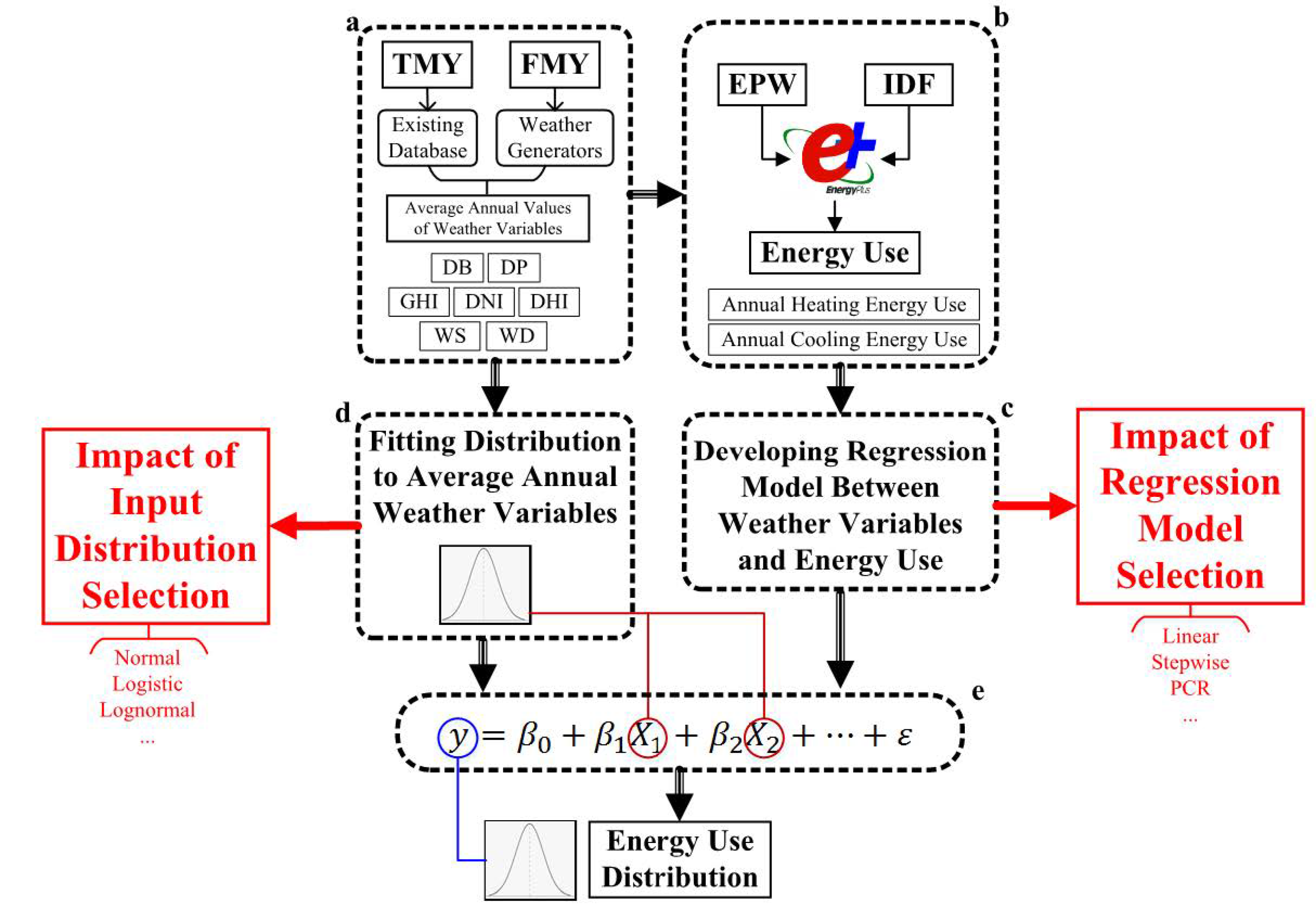
2.1. Study Approach
- Current and future weather files are created. Current weather files are obtained from existing resource presenting different historical periods. Future weather files are developed using weather generators (Step a in Figure 1).
- Multiple dynamic building simulations for each weather file is conducted and annual heating and cooling energy use are determined (Step b in Figure 1).
- The average annual values (arithmetic mean values) for each weather variable of the weather files are calculated and the corresponding principal components of the weather variables are developed.
- Regression models between the average annual weather variables (and principal components) as regressors and annual heating and cooling energy use (as dependent variables) are developed (Step c in Figure 1).
- Sample distributions are fit to the average annual weather variables of the weather files data sets and their corresponding principal components (Step d in Figure 1). The sample distribution is repeated for all weather variables and PCs except for the best fit scenario. For example, when the Erlang distribution is selected, all weather variables are assumed to follow an Erlang distribution.
- Parameters of the distributions are obtained and a random sampling of a sample size of 100 is conducted for all weather variables and principal components.
- The uncertainties of the input variables (weather variables and their associated principal components) are then propagated to the heating and cooling energy use using the regression model developed (Step e in Figure 1).
2.2. Case Study and Weather Files
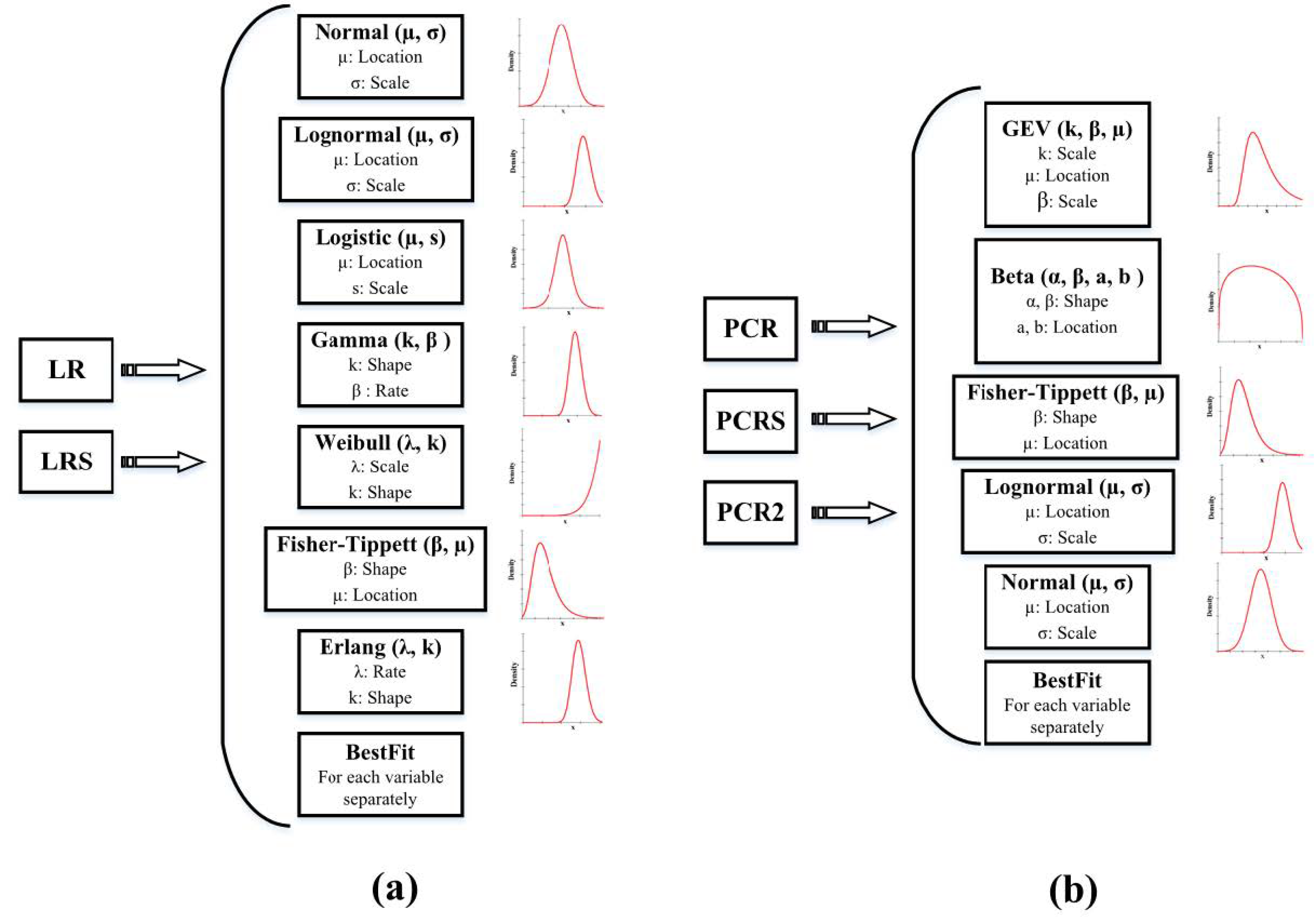
2.3. Selection of Regression Model
2.4. Selection of Average Annual Weather Variables Distributions
3. Results
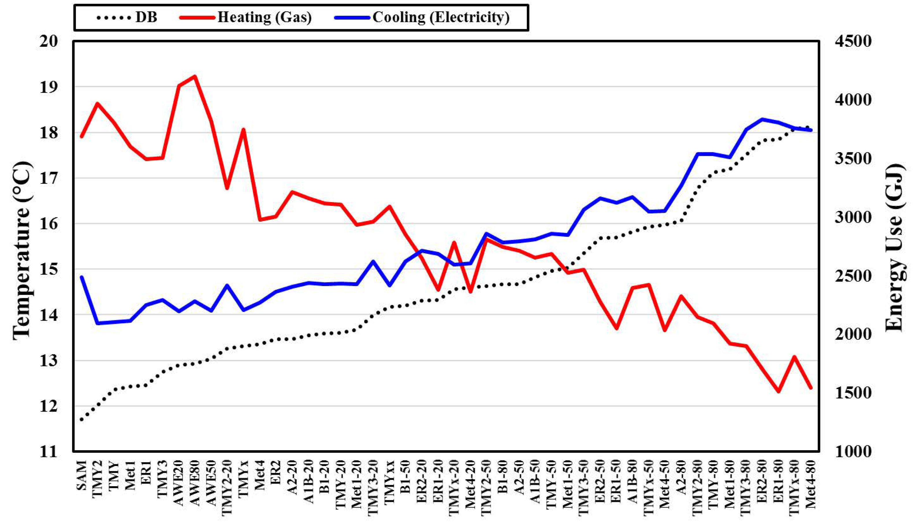
3.1. Summary of Current and Future Weather Data & Energy Use
3.2. Developed Regression Models
3.3. Input Variables Distributions
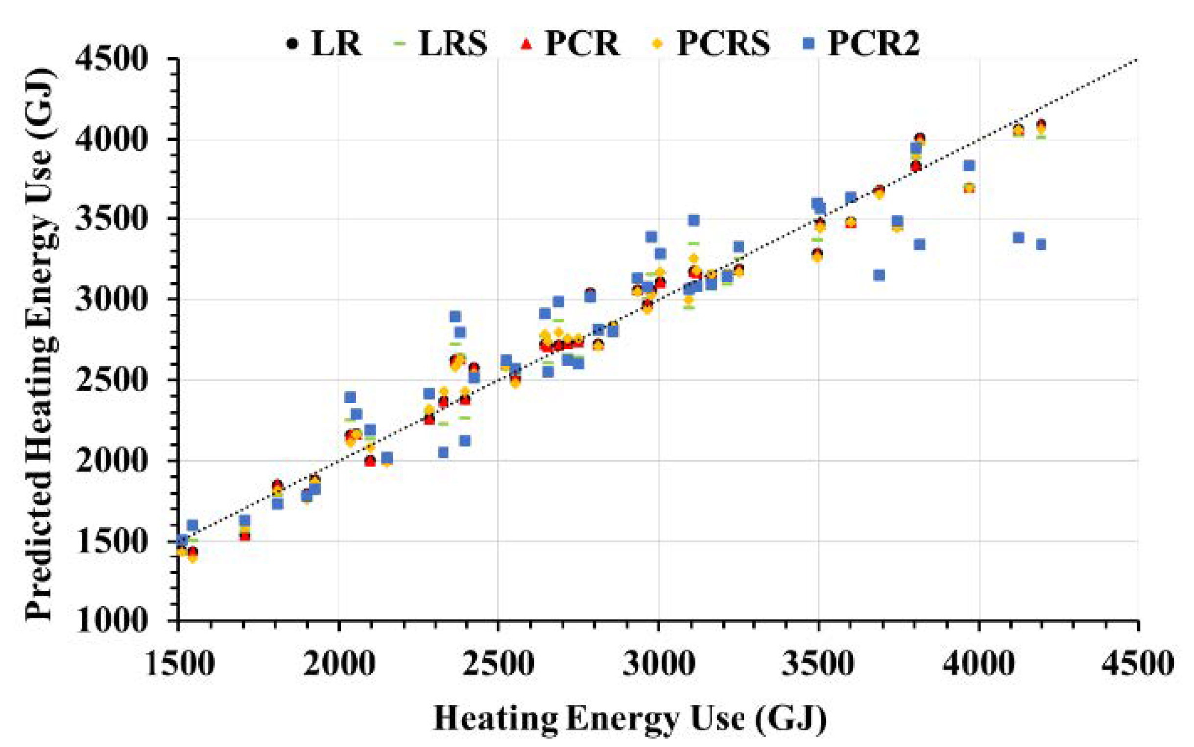
3.4. Impact of Regression Model Selection on Energy Use
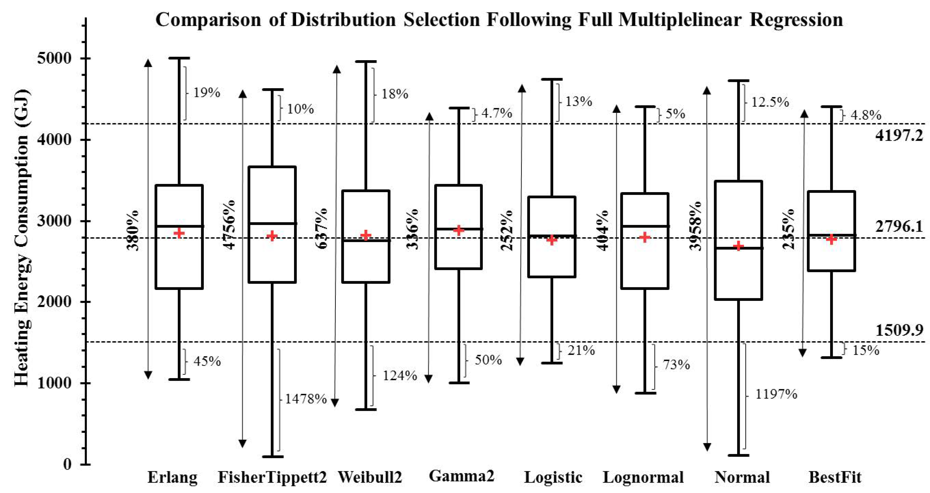
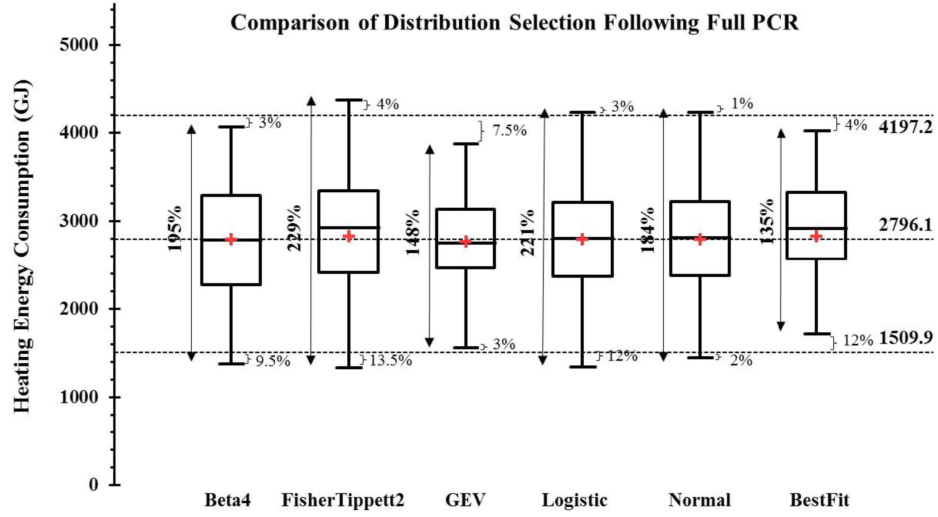
3.5. Impact Assessment of Regression Model and Input Average Annual Variables Distributions on Energy Use Distributions
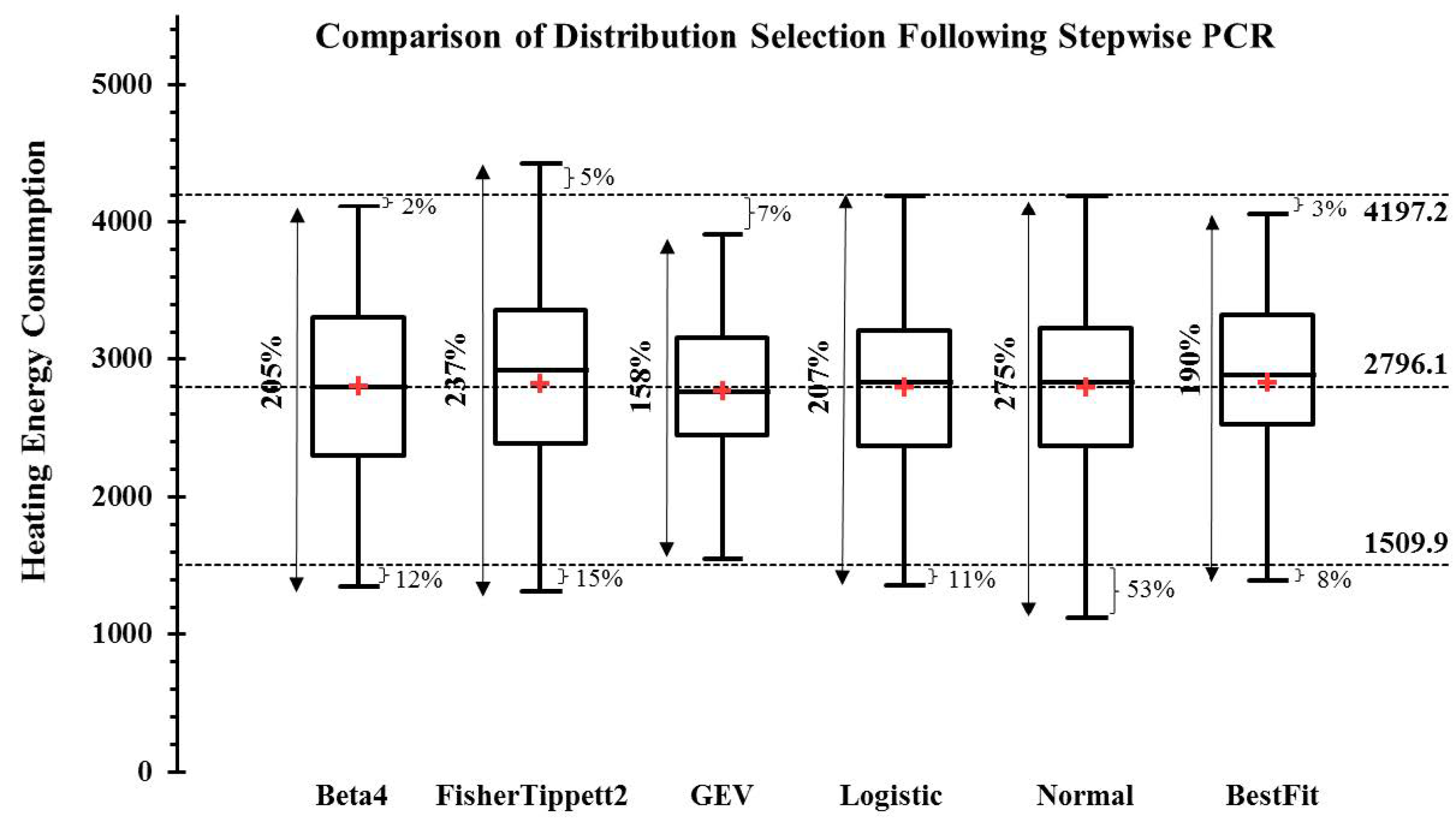
3.5.1. Impact Assessment on Heating Energy Use Distribution
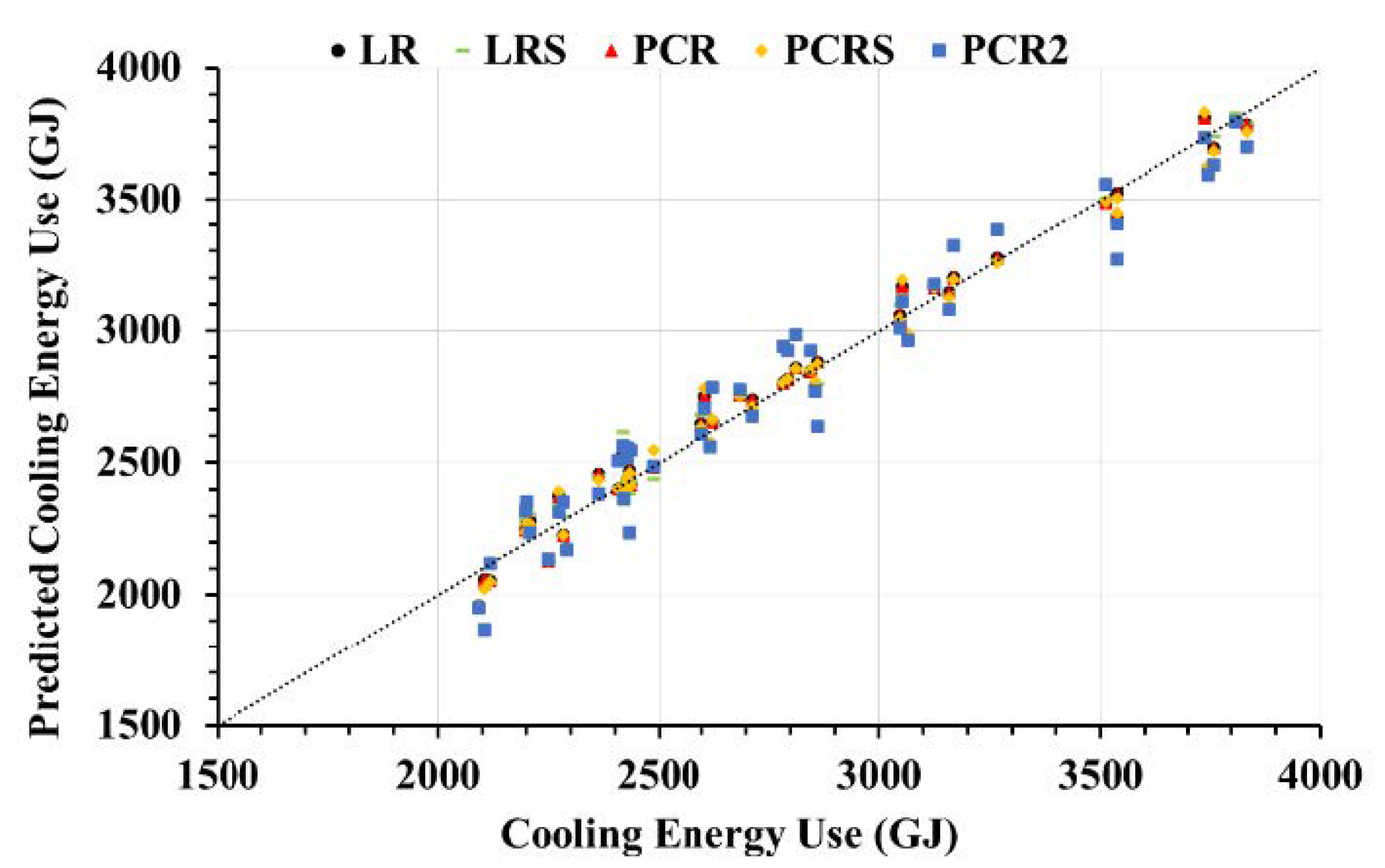
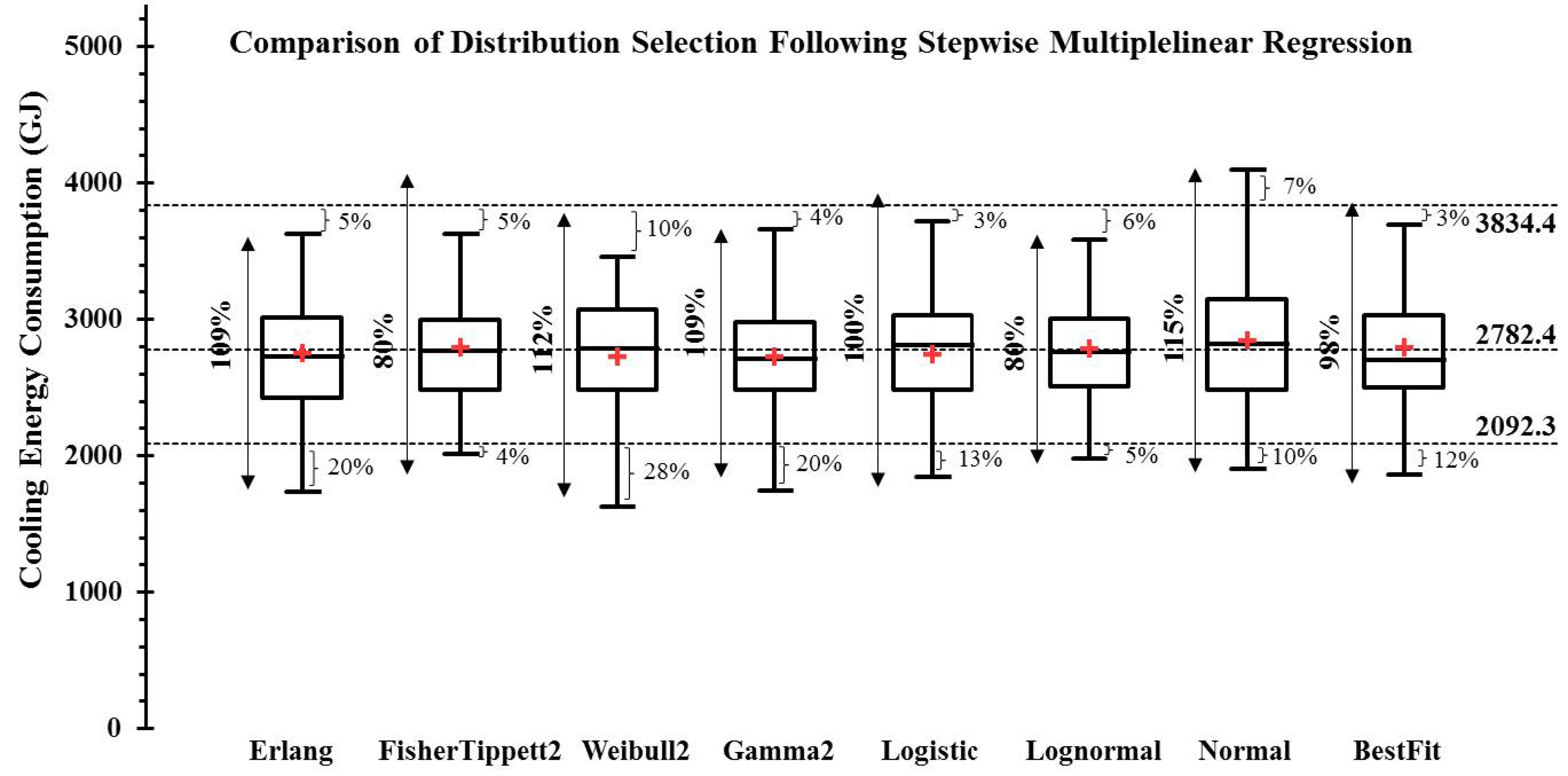
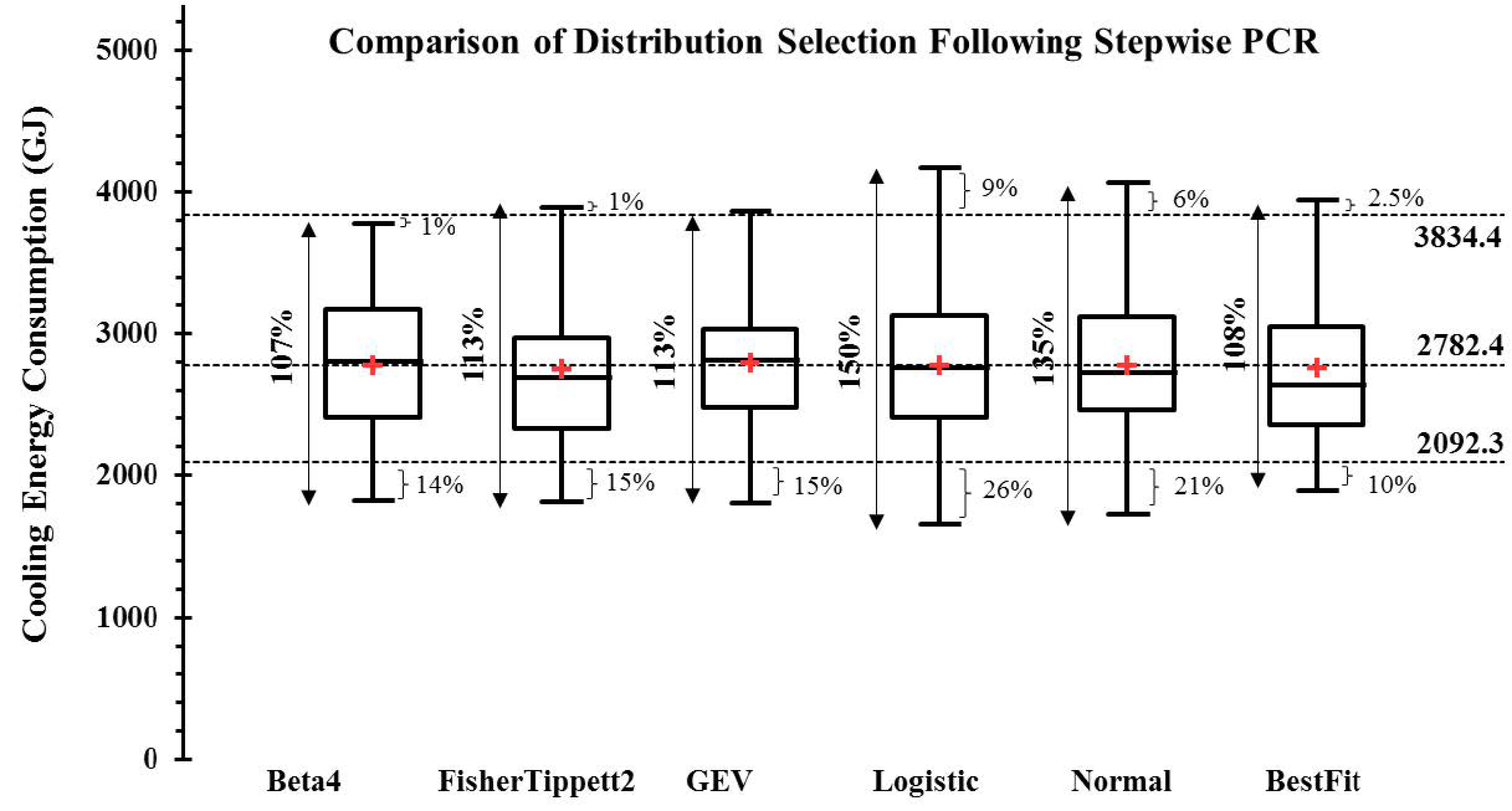
3.5.2. Impact Assessment on Cooling Energy Use Distribution
4. Discussion
5. Conclusions
Author Contributions
Funding
Institutional Review Board Statement
Informed Consent Statement
Data Availability Statement
Acknowledgments
Conflicts of Interest
Appendix A

| Current Weather Files | Future Weather Files | |||
|---|---|---|---|---|
| File | Source | Period | Method | Scenario(s) |
| TMY | National Solar Radiation Data Base | 1952–1975 | Advanced Weather Generator (AWE-GEN) | - |
| TMY2 | National Solar Radiation Data Base | 1961–1990 | Morphed TMY | A2 |
| TMY3 | National Solar Radiation Data Base | 1991–2005 | Morphed TMY2 | A2 |
| TMYx | Climate.OneBuilding.Org | 2003–2017 | Morphed TMY3 | A2 |
| TMYxx | Climate.OneBuilding.Org | 2004–2018 | Meteonorm | A1B, B1, A2 |
| ER1 | European Commission of Energy Efficiency Research | 2004–2014 | Morphed Met1 | A2 |
| ER2 | European Commission of Energy Efficiency Research | 2005–2015 | Morphed Met4 | A2 |
| Met1 | Meteonorm Base | 1961–1990 | Morphed TMYx | A2 |
| Met4 | Meteonorm Base | 2000–2009 | Morphed ER1 | A2 |
| SAM | System Advisor Model | 2010 | Morphed ER2 | A2 |
Appendix B
| Parameter | Unit | Large Office | |
|---|---|---|---|
| Wall | U-factor | W/m2-K | 0.857 |
| Roof | Type | - | IEAD 1 |
| U-factor | W/m2-K | 0.365 | |
| Floor | Type | - | Slab |
| U-factor | W/m2-K | 2.193 | |
| Window | U-value | W/m2-K | 3.241 |
| WWR2 | % | 40.00 | |
| SHGC3 | - | 0.385 | |
| Infiltration | - | m3/s-m2 | 0.302 × 10⁻⁴ |
| Outdoor Air | Requirement | m3/s-person | 0.0125 |
| Occupancy | Density | m2/person | 18.58 |
| PLD 2—LPD 3 | Interior | W/m2 | 10.76 |
| Fan | - | Control Type | VAV 4 |
| Efficiency | % | 60 | |
| Heating | Type | - | Boiler |
| Efficiency | % | 78 | |
| Cooling | Type | - | Chiller |
| Efficiency | COP | 5.5 |
Appendix C
| Weather Variables | Principal Components | Energy Use | ||||||||||||||
|---|---|---|---|---|---|---|---|---|---|---|---|---|---|---|---|---|
| Scenario | DB | DP | GHI | DNI | DHI | WD | WS | F1 | F2 | F3 | F4 | F5 | F6 | F7 | Heat. | Cool. |
| A1B-20 | 13.5 | 6.8 | 171.9 | 164.1 | 78.0 | 214.4 | 4.8 | 0.96 | −0.47 | 1.22 | −0.32 | 0.11 | 0.21 | −0.02 | 3161.5 | 2436.4 |
| A1B-50 | 14.8 | 8.1 | 172.3 | 166.1 | 77.9 | 215.7 | 4.8 | 0.79 | 0.76 | 0.93 | −0.34 | 0.12 | 0.36 | 0.14 | 2653.8 | 2810.8 |
| A1B-80 | 15.8 | 9.0 | 172.7 | 166.9 | 77.5 | 214.4 | 4.8 | 0.60 | 1.70 | 0.66 | −0.39 | 0.19 | 0.47 | 0.25 | 2397.3 | 3169.5 |
| A2-20 | 13.5 | 6.8 | 171.2 | 162.1 | 78.8 | 214.4 | 4.8 | 1.11 | −0.54 | 1.16 | −0.32 | 0.06 | 0.14 | 0.04 | 3212.6 | 2407.8 |
| A2-50 | 14.7 | 7.9 | 171.9 | 163.4 | 79.1 | 215.7 | 4.8 | 0.98 | 0.63 | 0.93 | −0.38 | 0.01 | 0.25 | 0.17 | 2714.9 | 2794.3 |
| A2-80 | 16.1 | 9.3 | 171.4 | 167.8 | 75.5 | 214.4 | 4.8 | 0.48 | 1.85 | 0.45 | −0.21 | 0.49 | 0.61 | 0.26 | 2324.0 | 3266.7 |
| AWE20 | 12.9 | 7.7 | 166.4 | 91.6 | 74.8 | 147.2 | 4.1 | 0.59 | −1.22 | −2.25 | −1.70 | 0.08 | 0.10 | −0.06 | 4121.6 | 2197.0 |
| AWE50 | 13.0 | 7.7 | 167.7 | 92.9 | 74.8 | 147.2 | 4.0 | 0.41 | −1.16 | −2.21 | −1.70 | −0.07 | 0.06 | −0.16 | 3815.0 | 2199.3 |
| AWE80 | 12.9 | 7.7 | 168.5 | 94.5 | 74.0 | 147.2 | 4.1 | 0.33 | −1.18 | −2.07 | −1.78 | 0.07 | 0.19 | −0.21 | 4197.2 | 2283.9 |
| B1-20 | 13.6 | 6.9 | 171.2 | 165.3 | 76.9 | 214.4 | 4.8 | 0.88 | −0.46 | 1.14 | −0.21 | 0.27 | 0.29 | −0.01 | 3116.8 | 2428.6 |
| B1-50 | 14.2 | 7.5 | 173.3 | 162.3 | 81.1 | 215.7 | 4.8 | 1.11 | 0.26 | 1.21 | −0.57 | −0.30 | 0.09 | 0.11 | 2855.1 | 2622.4 |
| B1-80 | 14.7 | 7.9 | 173.2 | 166.5 | 78.4 | 214.4 | 4.8 | 0.76 | 0.63 | 1.05 | −0.44 | 0.02 | 0.30 | 0.11 | 2747.6 | 2784.8 |
| ER1 | 12.5 | 5.2 | 179.2 | 195.7 | 69.1 | 147.1 | 3.7 | −2.57 | −2.46 | 0.88 | −0.32 | −0.15 | −0.47 | −0.12 | 3496.6 | 2249.6 |
| ER1-20 | 14.3 | 6.7 | 181.7 | 211.3 | 66.1 | 147.6 | 3.6 | −3.44 | −0.80 | 0.75 | −0.14 | 0.04 | −0.17 | −0.03 | 2381.4 | 2685.3 |
| ER1-50 | 15.7 | 7.7 | 182.9 | 213.5 | 65.4 | 147.6 | 3.6 | −3.78 | 0.28 | 0.50 | −0.11 | 0.06 | −0.15 | −0.05 | 2051.0 | 3124.8 |
| ER1-80 | 17.8 | 9.2 | 184.5 | 216.4 | 64.3 | 147.6 | 3.5 | −4.26 | 1.98 | 0.12 | −0.09 | 0.16 | −0.13 | −0.09 | 1509.9 | 3807.8 |
| ER2 | 13.5 | 6.2 | 173.4 | 188.6 | 65.8 | 145.8 | 3.9 | −2.33 | −1.68 | 0.04 | −0.05 | 0.74 | −0.20 | 0.16 | 3003.6 | 2362.7 |
| ER2-20 | 14.3 | 6.7 | 176.9 | 202.4 | 64.7 | 140.3 | 3.8 | −3.06 | −0.99 | 0.27 | −0.13 | 0.73 | −0.20 | 0.19 | 2645.9 | 2714.2 |
| ER2-50 | 15.7 | 7.6 | 178.0 | 204.3 | 64.0 | 140.3 | 3.7 | −3.39 | 0.09 | 0.01 | −0.10 | 0.75 | −0.18 | 0.16 | 2278.9 | 3158.8 |
| ER2-80 | 17.8 | 9.1 | 179.6 | 207.4 | 62.8 | 140.3 | 3.7 | −3.88 | 1.79 | −0.37 | −0.07 | 0.85 | −0.16 | 0.12 | 1705.3 | 3834.4 |
| Met1 | 12.4 | 5.7 | 169.0 | 157.5 | 79.9 | 215.7 | 4.8 | 1.54 | −1.57 | 1.27 | −0.20 | 0.02 | −0.07 | 0.01 | 3601.9 | 2117.9 |
| Met1-20 | 13.7 | 6.8 | 171.0 | 154.2 | 81.0 | 215.7 | 4.7 | 1.42 | −0.45 | 1.05 | −0.44 | −0.20 | −0.09 | −0.02 | 2933.4 | 2428.5 |
| Met1-50 | 15.0 | 7.8 | 172.1 | 156.6 | 80.1 | 215.7 | 4.7 | 1.05 | 0.65 | 0.77 | −0.39 | −0.19 | −0.05 | −0.04 | 2526.1 | 2845.7 |
| Met1-80 | 17.2 | 9.3 | 173.7 | 160.2 | 78.7 | 215.7 | 4.6 | 0.52 | 2.37 | 0.37 | −0.34 | −0.08 | 0.02 | −0.07 | 1923.8 | 3510.9 |
| Met4 | 13.4 | 6.2 | 167.6 | 156.4 | 79.9 | 215.7 | 4.2 | 1.07 | −1.12 | 0.44 | 0.42 | −0.60 | −0.35 | −0.03 | 2974.3 | 2273.3 |
| Met4-20 | 14.6 | 7.2 | 169.6 | 152.7 | 81.4 | 215.7 | 4.1 | 0.99 | 0.00 | 0.23 | 0.16 | −0.85 | −0.40 | −0.05 | 2365.1 | 2606.3 |
| Met4-50 | 16.0 | 8.2 | 170.8 | 154.9 | 80.6 | 215.7 | 4.1 | 0.64 | 1.09 | −0.04 | 0.20 | −0.84 | −0.38 | −0.07 | 2033.0 | 3053.2 |
| Met4-80 | 18.1 | 9.7 | 172.4 | 158.0 | 79.5 | 215.7 | 4.0 | 0.15 | 2.81 | −0.43 | 0.23 | −0.75 | −0.34 | −0.10 | 1542.9 | 3739.7 |
| SAM | 11.7 | 7.7 | 177.6 | 202.5 | 63.6 | 147.2 | 1.9 | −4.60 | −1.91 | −1.50 | 1.22 | −2.07 | 0.91 | 0.32 | 3690.7 | 2487.9 |
| TMY | 12.4 | 5.8 | 154.2 | 133.6 | 72.6 | 212.8 | 4.3 | 1.86 | −2.24 | −0.99 | 1.17 | 1.02 | 0.14 | 0.17 | 3804.9 | 2104.6 |
| TMY2 | 12.0 | 5.5 | 166.1 | 154.0 | 76.7 | 209.6 | 4.3 | 1.07 | −2.17 | 0.48 | 0.36 | −0.04 | −0.03 | −0.06 | 3968.1 | 2092.3 |
| TMY-20 | 13.6 | 6.7 | 156.2 | 128.4 | 79.3 | 212.8 | 4.3 | 2.29 | −1.07 | −1.00 | 0.67 | 0.26 | −0.34 | 0.41 | 3106.9 | 2431.7 |
| TMY2-20 | 13.3 | 6.6 | 168.1 | 146.9 | 80.9 | 209.6 | 4.3 | 1.27 | −0.93 | 0.26 | −0.07 | −0.61 | −0.22 | 0.07 | 3248.3 | 2418.8 |
| TMY2-50 | 14.6 | 7.6 | 169.2 | 149.0 | 80.1 | 209.6 | 4.2 | 0.92 | 0.17 | −0.02 | −0.04 | −0.60 | −0.18 | 0.05 | 2810.3 | 2855.9 |
| TMY2-80 | 16.8 | 9.2 | 170.8 | 152.1 | 78.8 | 209.6 | 4.1 | 0.42 | 1.91 | −0.42 | −0.01 | −0.50 | −0.13 | 0.02 | 2146.8 | 3538.3 |
| TMY3 | 12.7 | 5.9 | 167.7 | 161.0 | 74.3 | 206.6 | 4.2 | 0.44 | −1.68 | 0.37 | 0.49 | 0.04 | 0.03 | −0.15 | 3506.2 | 2291.0 |
| TMY3-20 | 14.0 | 6.9 | 169.7 | 154.6 | 77.8 | 206.6 | 4.1 | 0.57 | −0.52 | 0.17 | 0.12 | −0.43 | −0.15 | −0.10 | 2963.0 | 2618.9 |
| TMY3-50 | 15.4 | 7.9 | 170.8 | 156.7 | 76.9 | 206.6 | 4.1 | 0.21 | 0.57 | −0.11 | 0.16 | −0.41 | −0.12 | −0.13 | 2552.0 | 3064.6 |
| TMY3-80 | 17.5 | 9.4 | 172.4 | 159.5 | 75.7 | 206.6 | 4.0 | −0.28 | 2.29 | −0.50 | 0.18 | −0.31 | −0.07 | −0.16 | 1897.9 | 3745.8 |
| TMY-50 | 15.0 | 7.7 | 157.3 | 130.4 | 78.5 | 212.8 | 4.3 | 1.97 | 0.03 | −1.24 | 0.68 | 0.32 | −0.30 | 0.39 | 2688.4 | 2860.8 |
| TMY-80 | 17.1 | 9.2 | 158.9 | 133.4 | 77.2 | 212.8 | 4.2 | 1.48 | 1.75 | −1.63 | 0.70 | 0.44 | −0.24 | 0.36 | 2094.4 | 3538.1 |
| TMYx | 13.3 | 6.3 | 162.2 | 142.2 | 74.4 | 221.4 | 4.3 | 1.40 | −1.27 | −0.24 | 0.79 | 0.43 | 0.15 | −0.25 | 3746.5 | 2208.2 |
| TMYx-20 | 14.6 | 7.2 | 163.9 | 143.2 | 74.4 | 221.4 | 4.3 | 1.14 | −0.25 | −0.40 | 0.70 | 0.39 | 0.14 | −0.29 | 2785.3 | 2596.7 |
| TMYx-50 | 15.9 | 8.2 | 165.1 | 145.1 | 73.7 | 221.4 | 4.2 | 0.80 | 0.84 | −0.67 | 0.73 | 0.39 | 0.16 | −0.32 | 2423.9 | 3047.4 |
| TMYx-80 | 18.1 | 9.7 | 166.6 | 147.0 | 72.7 | 221.4 | 4.2 | 0.35 | 2.55 | −1.08 | 0.74 | 0.46 | 0.17 | −0.36 | 1807.1 | 3759.1 |
| TMYxx | 14.2 | 6.4 | 171.0 | 182.4 | 67.0 | 210.1 | 3.9 | −0.99 | −0.86 | 0.43 | 1.16 | 0.51 | 0.35 | −0.60 | 3091.0 | 2417.6 |
Appendix D
| Heating | Cooling | |
|---|---|---|
| LR | 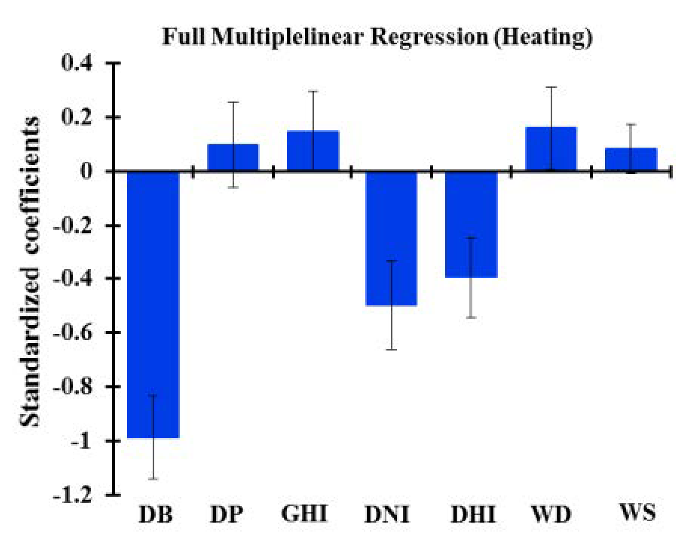 | 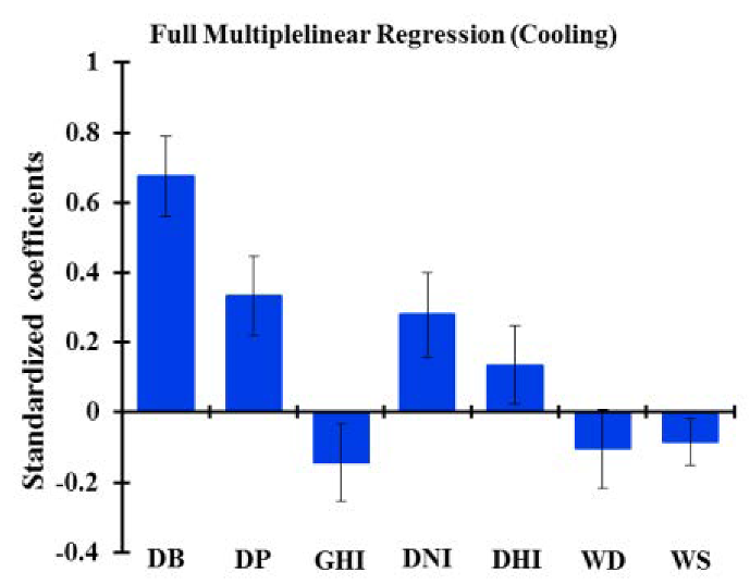 |
| LRS | 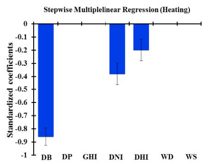 | 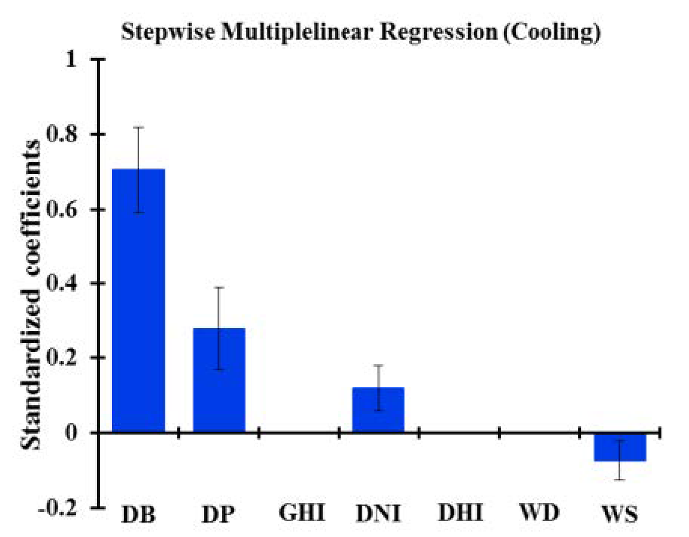 |
| PCRF | 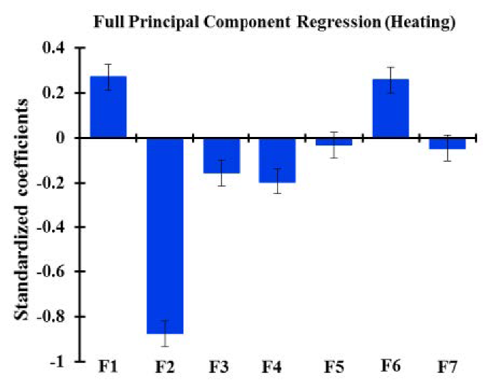 |  |
| PCRS |  |  |
| PCR2 |  |  |
Appendix E
| Cooling | Heating | |||||||
|---|---|---|---|---|---|---|---|---|
| Variable | Coeff. | Value | Std. error | Pr > |t| | Value | Std. error | Pr > |t| | |
| LR | Intercept | −294.329 | 564.078 | 0.605 | 9727.159 | 1020.073 | <0.0001 | |
| DB | 202.714 | 16.830 | <0.0001 | −396.019 | 30.435 | <0.0001 | ||
| DP | 145.703 | 25.119 | <0.0001 | 58.934 | 45.424 | 0.202 | ||
| GHI | −11.689 | 4.437 | 0.012 | 16.153 | 8.024 | 0.051 | ||
| DNI | 4.994 | 1.092 | <0.0001 | −11.924 | 1.975 | <0.0001 | ||
| DHI | 12.340 | 5.042 | 0.019 | −48.300 | 9.117 | <0.0001 | ||
| WD | −1.784 | 0.945 | 0.067 | 3.671 | 1.710 | 0.038 | ||
| WS | −88.557 | 34.102 | 0.013 | 114.733 | 61.671 | 0.071 | ||
| LRS | Intercept | −1260.904 | 170.992 | <0.0001 | 11147.753 | 497.251 | <0.0001 | |
| DB | 211.805 | 16.863 | <0.0001 | −344.807 | 13.134 | <0.0001 | ||
| DP | 121.489 | 23.818 | <0.0001 | 0.000 | 0.000 | - | ||
| GHI | 0.000 | 0.000 | - | 0.000 | 0.000 | - | ||
| DNI | 2.136 | 0.534 | 0.00 | −9.170 | 0.998 | <0.0001 | ||
| DHI | 0.00 | 0.000 | - | −24.446 | 4.990 | <0.0001 | ||
| WD | 0.00 | 0.000 | - | 0.000 | 0.000 | - | ||
| WS | −75.335 | 26.990 | 0.008 | 0.000 | 0.000 | - | ||
| PCR | Intercept | 2782.435 | 10.854 | <0.0001 | 2796.132 | 19.629 | <0.0001 | |
| F1 | −78.034 | 5.944 | <0.0001 | 101.503 | 10.748 | <0.0001 | ||
| F2 | 344.047 | 7.763 | <0.0001 | −430.372 | 14.039 | <0.0001 | ||
| F3 | −50.977 | 11.580 | <0.0001 | −114.421 | 20.941 | <0.0001 | ||
| F4 | 95.460 | 16.694 | <0.0001 | −206.575 | 30.189 | <0.0001 | ||
| F5 | 31.770 | 20.103 | 0.122 | −41.260 | 36.354 | 0.263 | ||
| F6 | −185.519 | 39.064 | <0.0001 | 635.965 | 70.642 | <0.0001 | ||
| F7 | 120.310 | 54.266 | 0.033 | −157.836 | 98.134 | 0.116 | ||
| PCRS | Intercept | 2782.435 | 11.061 | <0.0001 | 2796.132 | 20.084 | <0.0001 | |
| F1 | −78.034 | 6.057 | <0.0001 | 101.503 | 10.997 | <0.0001 | ||
| F2 | 344.047 | 7.911 | <0.0001 | −430.372 | 14.364 | <0.0001 | ||
| F3 | −50.977 | 11.800 | 0.000 | −114.421 | 21.426 | <0.0001 | ||
| F4 | 95.460 | 17.012 | <0.0001 | −206.575 | 30.889 | <0.0001 | ||
| F5 | 0.000 | 0.000 | - | 0.000 | 0.000 | - | ||
| F6 | −185.519 | 39.806 | <0.0001 | 635.965 | 72.279 | <0.0001 | ||
| F7 | 120.310 | 55.298 | 0.036 | 0.000 | 0.000 | - | ||
| Intercept | 2782.435 | 18.136 | <0.0001 | 2796.132 | 42.290 | <0.0001 | ||
| PCR2 | F1 | −78.034 | 9.931 | <0.0001 | 101.503 | 23.157 | <0.0001 | |
| F2 | 344.047 | 12.971 | <0.0001 | −430.372 | 30.246 | <0.0001 | ||
Appendix F
| Distribution | Var. | Parameter(s) [Standard Error] | Var. | Parameter(s) [Standard Error] | ||
|---|---|---|---|---|---|---|
| Normal (µ, σ) µ: Location σ: Scale | DB | (14.65 [0.18], 1.1716 [0.188]) | F1 | (0.00 [0.265], 1.826 [0.188]) | ||
| DP | (7.53 [0.171], 1.17 [0.125]) | F2 | (0.00 [0.210], 1.397 [0.146]) | |||
| GHI | (170.48 [-], 6.34 [-]) | F3 | (0.00 [0.138], 0.937 [0.097]) | |||
| DNI | (160.33 [0.265], 28.606 [0.42]) | F4 | (0.00 [0.096], 0.65 [0.068]) | |||
| DHI | (74.88 [0.42], 5.59 [0.34]) | F5 | (0.00 [0.08], 0.54 [0.056]) | |||
| WD | (196.001 [0.198], 30.27 [0.59]) | F6 | (0.00 [0.041], 0.278 [0.029]) | |||
| WS | (4.197 [0.074], 0.501 [0.05]) | F7 | (0.00 [0.029], 0.199 [0.021]) | |||
| Lognormal (µ, σ) µ: Location σ: Scale | DB | (2.68 [0.016], 0.115 [0.012]) | ||||
| DP | (2.006 [0.023], 0.158 [0.016]) | |||||
| GHI | (5.138 [0.006], 0.038 [0.004]) | |||||
| DNI | (5.06 [0.028], 0.19 [0.02]) | |||||
| DHI | (4.313 [0.01], 0.078 [0.008]) | |||||
| WD | (5.26 [0.025], 0.17 [0.018]) | |||||
| WS | (1.125 [0.021], 0.145 [0.015]) | |||||
| Logistic (µ, s) µ: Location s: Scale | DB | (14.53 [0.26], 1.002 [0.13]) | F1 | (0.362 [0.205], 0.946 [0.126]) | ||
| DP | (7.49 [0.18], 0.69 [0.08]) | F2 | (−0.062 [0.253], 0.831 [0.103]) | |||
| GHI | (170.65 [-], 3.40 [1.18]) | F3 | (0.091 [0.142], 0.531 [0.066]) | |||
| DNI | (159.88 [0.61], 15.39 [0.61]) | F4 | Fitted Normal | |||
| DHI | (75.69 [0.42], 3.16 [0.27]) | F5 | Fitted Normal | |||
| WD | (202.12 [0.26], 16.94 [0.22]) | F6 | (−0.019 [0.04], 0.155 [0.019]) | |||
| WS | Fitted Normal | F7 | (0.000 [0.028], 0.111 [0.014]) | |||
| Gamma (k, β) k: Shape β: Rate | DB | (74.59 [15.55], 0.19 [0.04]) | ||||
| DP | (40.49 [8.44], 0.18 [0.04]) | |||||
| GHI | (705.91 [147.19], 0.24 [0.05]) | |||||
| DNI | (29.09 [6.068], 5.51 [1.16]) | |||||
| DHI | (170.58 [35.64], 0.44 [0.09]) | |||||
| WD | (36.9 [7.68], 5.31 [1.11]) | |||||
| WS | (55.26 [11.51], 0.07 [0.016]) | |||||
| Weibull (λ, k) λ: Scale k: Shape | DB | (8.79 [0.00], 15.43 [1.162]) | ||||
| DP | (7.016 [0.61], 8.04 [0.17]) | |||||
| GHI | (28.72 [0.34], 173.47 [0.11]) | |||||
| DNI | (6.19 [-], 172.14 [0.19]) | |||||
| DHI | (18.97 [0.59], 77.26 [0.13]) | |||||
| WD | (9.88 [0.59], 207.9 [0.59]) | |||||
| WS | 11.86 [0.94], 4.39 [0.05]) | |||||
| Fisher-Tippett (β, µ) µ: Location β: Shape | DB | (1.42 [0.22], 13.83 [0.16]) | F1 | (2.156 [0.34], −1.013 [0.223]) | ||
| DP | (1.07 [0.17], 6.95 [0.12]) | F2 | (1.212 [0.189], −0.677 [0.139]) | |||
| GHI | (6.85 [1.07], 162.2 [0.70]) | F3 | (1.039 [0.163], −0.501 [0.108]) | |||
| DNI | (30.26 [7.74], 145.76 [3.09]) | F4 | (0.762 [0.12], −0.346 [0.075]) | |||
| DHI | (6.12 [0.96], 71.87 [0.65]) | F5 | (0.426 [0.071, −0.246 [0.017]) | |||
| WD | (32.93 [5.17], 179.52 [3.58]) | F6 | (0.226 [0.035, −0.129 [0.026]) | |||
| WS | (0.76 [0.12], 3.90 [0.67]) | F7 | (0.218 [0.034], −0.102 [0.022]) | |||
| Erlang (k, λ) k: Shape λ: Rate | DB | (71.0 [0.14], 4.863 [0.08]) | - | - | ||
| DP | (39.0 [0.14], 5.312 [0.12]) | - | - | |||
| GHI | (705.0 [0.15], 4.141 [0.02]) | - | - | |||
| DNI | (30.0 [0.14], 0.192 [0.005]) | - | - | |||
| DHI | (175.0 [0.15], 2.344 [0.02]) | - | - | |||
| WD | (40.0 [0.14], 0.209 [0.005]) | - | - | |||
| WS | (68.0 [0.14], 16.373 [0.29]) | - | - | |||
| Chi-square (DF) DF: Degree of Freedom | DB | (15.538 [0.245]) | - | - | ||
| DP | (8.414 [0.305]) | - | - | |||
| GHI | (171.346 [0.211]) | - | - | |||
| DNI | (158.583 [0.211]) | - | - | |||
| DHI | (75.66 [0.214]) | - | - | |||
| WD | (194.35 [0.211]) | - | - | |||
| WS | (5.12 [0.944]) | - | - | |||
| GEV (k, β, µ) k: Scale β: Shape µ: Location | F1 | (−0.74 [0.001], 1.88 [0.004], −0.22 [0.005]) | ||||
| F2 | (−0.197 [0.15], 1.293 [0.18], −0.54 [0.22]) | |||||
| F3 | (−0.77 [0.003], 1.07 [0.003], −0.1 [0.004]) | |||||
| F4 | (−0.43 [0.04], 0.7 [0.036], −0.18 [0.05]) | |||||
| F5 | (−0.47 [0.02], 0.58 [0.017], −0.14 [0.24]) | |||||
| F6 | (−0.04 [0.102], 0.23 [0.026], −0.12 [0.036]) | |||||
| F7 | (−0.35 [0.12], 0.208 [0.03], −0.06 [0.046]) | |||||
| Beta (α, β, a, b) α, β: Shape a, b: Location | F1 | (337.92 [35.76], 1.845 [0.026], −438.636 [3.51], 2.37 [-]) | ||||
| F2 | (1.205 [0.026], 1.329 [0.028], −2.51 [-], 2.862 [-]) | |||||
| F3 | (4.006 [0.35], 1.21 [0.02], −4.11 [0.26], 1.306 [-]) | |||||
| F4 | (44.65 [1.67], 9.41 [0.068], −10.51 [0.214], 2.214 [0.136]) | |||||
| F5 | (220.62 [7.66], 7.43 [0.058], −44.27 [0.43], 1.49 [0.095]) | |||||
| F6 | (2.88 [0.044], 12.13 [0.122], −0.54 [0.023], 2.282 [0.21]) | |||||
| F7 | (26.37 [0.46], 15.89 [0.075], −1.7 [0.04], 1.024 [0.035]) | |||||
Appendix G
| Var. | Best Fit Selection | p-value | Next Three Fits |
|---|---|---|---|
| F1 | Beta4 | 0.036 | Gumbel, Logistic, GEV |
| F2 | Fisher-Tippett 2 | 0.851 | GEV, Logistic, Normal |
| F3 | Logistic | 0.736 | Fisher-Tippett2, Gumbel, Normal |
| F4 | Beta4 | 0.233 | Fisher-Tippet2, GEV, Normal |
| F5 | Beta4 | 0.860 | GEV, Normal |
| F6 | Beta4 | 0.982 | Fisher-Tippett2, Logistic, GEV |
| F7 | Normal | 0.914 | Beta4, Fisher-Tippett2, Logistic |
| DB | Fisher-Tippett 2 | 0.984 | Erlang, Lognormal, Logistic |
| DP | Lognormal | 0.592 | Logistic, Normal, Gamma2 |
| GHI | Logistic | 0.55 | Erlang, Lognormal, Normal |
| DNI | Chisquare | 0.299 | Lognormal, Logistic, Fisher-Tippett2 |
| DHI | Weibull2 | 0.376 | Logistic, Lognormal, Normal |
| WD | Normal | 0.00027 | - |
| WS | Normal | 0.396 | Erlang, Lognormal, Gamma2 |
References
- Šujanová, P.; Rychtáriková, M.; Mayor, T.S.; Hyder, A. A Healthy, Energy-Efficient and Comfortable Indoor Environment, a Review. Energies 2019, 12, 1414. [Google Scholar] [CrossRef] [Green Version]
- Tian, W.; Heo, Y.; De Wilde, P.; Li, Z.; Yan, D.; Park, C.S.; Feng, X.; Augenbroe, G. A review of uncertainty analysis in building energy assessment. Renew. Sustain. Energy Rev. 2018, 93, 285–301. [Google Scholar] [CrossRef] [Green Version]
- Meacham, B.J. Sustainability and resiliency objectives in performance building regulations. Build. Res. Inf. 2016, 44, 474–489. [Google Scholar] [CrossRef]
- Escandón, R.; Suárez, R.; Sendra, J.J.; Ascione, F.; Bianco, N.; Mauro, G.M. Predicting the Impact of Climate Change on Thermal Comfort in A Building Category: The Case of Linear-type Social Housing Stock in Southern Spain. Energies 2019, 12, 2238. [Google Scholar] [CrossRef] [Green Version]
- Hallegatte, S. Strategies to adapt to an uncertain climate change. Glob. Environ. Chang. 2009, 19, 240–247. [Google Scholar] [CrossRef]
- Yassaghi, H.; Mostafavi, N.; Hoque, S. Evaluation of current and future hourly weather data intended for building designs: A Philadelphia case study. Energy Build. 2019, 199, 491–511. [Google Scholar] [CrossRef]
- Bueno, B.; Norford, L.; Hidalgo, J.; Pigeon, G. The urban weather generator. J. Build. Perform. Simul. 2013, 6, 269–281. [Google Scholar] [CrossRef]
- Belcher, S.; Hacker, J.; Powell, D. Constructing design weather data for future climates. Build. Serv. Eng. Res. Technol. 2005, 26, 49–61. [Google Scholar] [CrossRef]
- Khan, M.S.; Coulibaly, P.; Dibike, Y. Uncertainty analysis of statistical downscaling methods. J. Hydrol. 2006, 319, 357–382. [Google Scholar] [CrossRef]
- Goodess, C.; Hanson, C.; Hulme, M.; Osborn, T. Representing Climate and Extreme Weather Events in Integrated Assessment Models: A Review of Existing Methods and Options for Development. Integr. Assess. 2003, 4, 145–171. [Google Scholar] [CrossRef]
- Nik, V.M.; Kalagasidis, A.S. Impact study of the climate change on the energy performance of the building stock in Stockholm considering four climate uncertainties. Build. Environ. 2013, 60, 291–304. [Google Scholar] [CrossRef]
- Yassaghi, H.; Hoque, S. An Overview of Climate Change and Building Energy: Performance, Responses and Uncertainties. Buildings 2019, 9, 166. [Google Scholar] [CrossRef] [Green Version]
- Belazi, W.; Ouldboukhitine, S.-E.; Chateauneuf, A.; Bouchair, A.; Bouchair, H. Uncertainty analysis of occupant behavior and building envelope materials in office building performance simulation. J. Build. Eng. 2018, 19, 434–448. [Google Scholar] [CrossRef]
- Gaetani, I.I.; Hoes, P.P.-J.; Hensen, J.J. On the sensitivity to different aspects of occupant behaviour for selecting the appropriate modelling complexity in building performance predictions. J. Build. Perform. Simul. 2016, 10, 601–611. [Google Scholar] [CrossRef] [Green Version]
- IPCC. 2014: Climate Change 2014: Synthesis Report. Contribution of Working Groups I, II and III to the Fifth Assessment Report of the Intergovernmental Panel on Climate Change; Core Writing Team, Pachauri, R.K., Meyer, L.A., Eds.; IPCC: Geneva, Switzerland, 2014; p. 151. [Google Scholar]
- Martinez-Soto, A.; Jentsch, M.F. A transferable energy model for determining the future energy demand and its uncertainty in a country’s residential sector. Build. Res. Inf. 2019, 48, 587–612. [Google Scholar] [CrossRef]
- Bortolini, R.; Forcada, N. A probabilistic performance evaluation for buildings and constructed assets. Build. Res. Inf. 2020, 48, 838–855. [Google Scholar] [CrossRef]
- Eisenhower, B.; O’Neill, Z.; Fonoberov, V.A.; Mezić, I. Uncertainty and sensitivity decomposition of building energy models. J. Build. Perform. Simul. 2012, 5, 171–184. [Google Scholar] [CrossRef]
- Cecconi, F.R.; Manfren, M.; Tagliabue, L.C.; Ciribini, A.L.C.; De Angelis, E. Probabilistic behavioral modeling in building performance simulation: A Monte Carlo approach. Energy Build. 2017, 148, 128–141. [Google Scholar] [CrossRef]
- Nik, V.M. Making energy simulation easier for future climate—Synthesizing typical and extreme weather data sets out of regional climate models (RCMs). Appl. Energy 2016, 177, 204–226. [Google Scholar] [CrossRef]
- Shen, P. Impacts of climate change on U.S. building energy use by using downscaled hourly future weather data. Energy Build. 2017, 134, 61–70. [Google Scholar] [CrossRef]
- Rodríguez, G.C.; Andrés, A.C.; Muñoz, F.D.; López, J.M.C.; Zhang, Y. Uncertainties and sensitivity analysis in building energy simulation using macroparameters. Energy Build. 2013, 67, 79–87. [Google Scholar] [CrossRef]
- Tian, W.; de Wilde, P. Uncertainty and sensitivity analysis of building performance using probabilistic climate projections: A UK case study. Autom. Constr. 2011, 20, 1096–1109. [Google Scholar] [CrossRef]
- Sun, Y.; Heo, Y.; Tan, M.; Xie, H.; Wu, C.J.; Augenbroe, G. Uncertainty quantification of microclimate variables in building energy models. J. Build. Perform. Simul. 2013, 7, 17–32. [Google Scholar] [CrossRef]
- Gang, W.; Wang, S.; Shan, K.; Gao, D. Impacts of cooling load calculation uncertainties on the design optimization of building cooling systems. Energy Build. 2015, 94, 1–9. [Google Scholar] [CrossRef]
- De Wilde, P.; Tian, W. Predicting the performance of an office under climate change: A study of metrics, sensitivity and zonal resolution. Energy Build. 2010, 42, 1674–1684. [Google Scholar] [CrossRef]
- Wang, L.; Mathew, P.; Pang, X. Uncertainties in energy consumption introduced by building operations and weather for a medium-size office building. Energy Build. 2012, 53, 152–158. [Google Scholar] [CrossRef] [Green Version]
- González, V.G.; Colmenares, L.Á.; López-Fidalgo, J.; Ruiz, G.R.; Bandera, C.F. Uncertainy’s Indices Assessment for Calibrated Energy Models. Energies 2019, 12, 2096. [Google Scholar] [CrossRef] [Green Version]
- Brohus, H.; Frier, C.; Heiselberg, P.; Haghighat, F. Quantification of uncertainty in predicting building energy consumption: A stochastic approach. Energy Build. 2012, 55, 127–140. [Google Scholar] [CrossRef] [Green Version]
- Fabrizio, E.; Monetti, V. Methodologies and Advancements in the Calibration of Building Energy Models. Energies 2015, 8, 2548–2574. [Google Scholar] [CrossRef] [Green Version]
- Braun, M.; Altan, H.; Beck, S. Using regression analysis to predict the future energy consumption of a supermarket in the UK. Appl. Energy 2014, 130, 305–313. [Google Scholar] [CrossRef] [Green Version]
- Catalina, T.; Iordache, V.; Caracaleanu, B. Multiple regression model for fast prediction of the heating energy demand. Energy Build. 2013, 57, 302–312. [Google Scholar] [CrossRef]
- Yassaghi, H.; Gurian, P.L.; Hoque, S. Propagating downscaled future weather file uncertainties into building energy use. Appl. Energy 2020, 278, 115655. [Google Scholar] [CrossRef]
- Ivanov, V.; Bras, R.L.; Curtis, D.C. A weather generator for hydrological, ecological, and agricultural applications. Water Resour. Res. 2007, 43. [Google Scholar] [CrossRef] [Green Version]
- Fatichi, S.; Ivanov, V.; Caporali, E. Simulation of future climate scenarios with a weather generator. Adv. Water Resour. 2011, 34, 448–467. [Google Scholar] [CrossRef]
- Peleg, N.; Fatichi, S.; Paschalis, A.; Molnar, P.; Burlando, P. An advanced stochastic weather generator for simulating 2-D high-resolution climate variables. J. Adv. Model. Earth Syst. 2017, 9, 1595–1627. [Google Scholar] [CrossRef]
- Jentsch, M.F.; James, P.A.B.; Bourikas, L.; Bahaj, A.S. Transforming existing weather data for worldwide locations to enable energy and building performance simulation under future climates. Renew. Energy 2013, 55, 514–524. [Google Scholar] [CrossRef]
- Chen, Y.; Wen, J. Whole Building System Fault Detection Based on Weather Pattern Matching and PCA Method; Institute of Electrical and Electronics Engineers (IEEE); China Agricultural University: Beijing, China, 2017; pp. 728–732. [Google Scholar]
- Wang, E. Benchmarking whole-building energy performance with multi-criteria technique for order preference by similarity to ideal solution using a selective objective-weighting approach. Appl. Energy 2015, 146, 92–103. [Google Scholar] [CrossRef]
- Devore, J.L.; Farnum, N.R.; Doi, J. Applied Statistics for Engineers and Scientists; Nelson Education: Scarborough, ON, Canada, 2013. [Google Scholar]


| Cooling | Heating | ||||||
|---|---|---|---|---|---|---|---|
| Variable | Coeff. | LR | LRS | LR | LRS | ||
| Intercept | −294.329 | −1260.9 | 9727.159 | 11147.75 | |||
| DB | 202.714 | 211.805 | −396.019 | −344.807 | |||
| DP | 145.703 | 121.489 | 58.934 | 0 | |||
| GHI | −11.689 | 0 | 16.153 | 0 | |||
| DNI | 4.994 | 2.136 | −11.924 | −9.17 | |||
| DHI | 12.34 | 0 | −48.3 | −24.446 | |||
| WD | −1.784 | 0 | 3.671 | 0 | |||
| WS | −88.557 | −75.335 | 114.733 | 0 | |||
| Variable | Coeff. | PCR | PCRS | PCR2 | PCR | PCRS | PCR2 |
| Intercept | 2782.435 | 2782.435 | 2782.435 | 2796.132 | 2796.132 | 2796.132 | |
| F1 | −78.034 | −78.034 | −78.034 | 101.503 | 101.503 | 101.503 | |
| F2 | 344.047 | 344.047 | 344.047 | −430.372 | −430.372 | −430.372 | |
| F3 | −50.977 | −50.977 | 0 | −114.421 | −114.421 | 0 | |
| F4 | 95.46 | 95.46 | 0 | −206.575 | −206.575 | 0 | |
| F5 | 31.77 | 0 | 0 | −41.26 | 0 | 0 | |
| F6 | −185.519 | −185.519 | 0 | 635.965 | 635.965 | 0 | |
| F7 | 120.31 | 120.31 | 0 | −157.836 | 0 | 0 | |
| Heating | Erlang | FisherTippett2 | Weibull2 | Gamma2 | Logistic | Lognormal | Normal | BestFit | Sum | Avg. |
|---|---|---|---|---|---|---|---|---|---|---|
| LR | 720.2 | 818.4 | 687.8 | 612.9 | 648.8 | 665.2 | 823.0 | 672.8 | 5649.0 | 706.1 |
| LRS | 567.3 | 610.3 | 581.8 | 477.3 | 516.7 | 515.1 | 650.8 | 557.9 | 4477.3 | 559.7 |
| Heating | Beta4 | FisherTippett2 | GEV | Logistic | Normal | BestFit | Sum | Average |
|---|---|---|---|---|---|---|---|---|
| PCR | 538.4 | 579.8 | 452.2 | 532.3 | 513.0 | 536.2 | 3152.0 | 525.3 |
| PCRS | 541.2 | 584.1 | 456.2 | 530.7 | 511.7 | 529.8 | 3153.6 | 525.6 |
| PCR2 | 504.3 | 540.8 | 444.8 | 503.0 | 494.8 | 517.1 | 3004.9 | 500.8 |
| Cooling | Erlang | FisherTippett2 | Weibull2 | Gamma2 | Logistic | Lognormal | Normal | BestFit | Sum | Avg. |
|---|---|---|---|---|---|---|---|---|---|---|
| LR | 390.3 | 405.3 | 355.4 | 306.8 | 365.0 | 321.2 | 402.1 | 355.4 | 2901.5 | 362.7 |
| LRS | 340.0 | 339.0 | 348.4 | 275.0 | 338.2 | 277.6 | 365.3 | 352.0 | 2635.5 | 329.4 |
| Cooling | Beta4 | FisherTippett2 | GEV | Logistic | Normal | BestFit | Sum | Average |
|---|---|---|---|---|---|---|---|---|
| PCR | 417.0 | 420.3 | 364.8 | 408.1 | 415.9 | 426.2 | 2452.4 | 408.7 |
| PCRS | 418.4 | 420.5 | 363.5 | 410.0 | 413.7 | 425.7 | 2451.8 | 408.6 |
| PCR2 | 402.1 | 429.5 | 354.4 | 401.1 | 394.2 | 412.2 | 2393.6 | 398.9 |
Publisher’s Note: MDPI stays neutral with regard to jurisdictional claims in published maps and institutional affiliations. |
© 2021 by the authors. Licensee MDPI, Basel, Switzerland. This article is an open access article distributed under the terms and conditions of the Creative Commons Attribution (CC BY) license (http://creativecommons.org/licenses/by/4.0/).
Share and Cite
Yassaghi, H.; Hoque, S. Impact Assessment in the Process of Propagating Climate Change Uncertainties into Building Energy Use. Energies 2021, 14, 367. https://doi.org/10.3390/en14020367
Yassaghi H, Hoque S. Impact Assessment in the Process of Propagating Climate Change Uncertainties into Building Energy Use. Energies. 2021; 14(2):367. https://doi.org/10.3390/en14020367
Chicago/Turabian StyleYassaghi, Hamed, and Simi Hoque. 2021. "Impact Assessment in the Process of Propagating Climate Change Uncertainties into Building Energy Use" Energies 14, no. 2: 367. https://doi.org/10.3390/en14020367