Interturn Short-Circuit Fault Detection of a Five-Phase Permanent Magnet Synchronous Motor

Abstract

Interturn short circuits are a common fault of permanent magnet synchronous motors (PMSMs). This paper proposes a new method to detect the interturn short-circuit fault (ISCF) of a five-phase PMSM. The method first takes the command voltage and measured current of each phase winding as the original signal and then obtains the delay signal orthogonal to the original signal via Hilbert transform. Then, the generalized instantaneous reactive power of each phase can be calculated from the orthogonal voltage and current signals of each phase. Finally, the influence of the ISCF on the generalized instantaneous reactive power of each phase is analyzed under different working conditions. By comparing the difference in the generalized instantaneous reactive power of each phase, it can be determined which phase winding has the ISCF. The proposed method is verified by simulated and experimental results.

1. Introduction

The five-phase permanent magnet synchronous motor (PMSM) has been widely used in fields with high reliability requirements due to its small size, high power density, simple structure, and strong fault tolerance [1,2]. However, during long-term operation, a PMSM is liable to experience various types of faults; an interturn short-circuit fault (ISCF) is one of the most common types of faults. Failure in timely detection may lead to phase-to-phase short circuits and permanent magnet demagnetization, eventually completely damaging the motor. Therefore, interturn short-circuit fault (ISCF) detection is highly necessary [3,4,5,6].

At present, there are three major approaches for the detection of ISCFs in PMSMs. The first approach is the signal-based method, which involves analyzing the selected signal and determining the characteristics of the ISCF [7,8,9]. This method mainly involves stator current analysis, stator current Parker’s vector analysis, and q-axis current analysis. Through frequency analysis of the collected current signals, a fault characteristic quantity can be determined to detect whether there is an ISCF [10,11,12]. Glowacz A. proposed a technique for fault diagnosis based on the recognition of currents. The original method of feature extraction called Method of Selection of Amplitudes of Frequencies–Ratio 15% of maximum of amplitude (MSAF-RATIO15) was analyzed. A classification of feature vectors was then performed using the Bayes classifier, Linear Discriminant Analysis (LDA), and Nearest Neighbor classifier [13]. The second approach is the model-based method, which relies on mathematical models and machine parameters [14,15,16]. State estimation and parameter estimation are mainly adopted to identify faults. Wu F. calculated the stator three-phase current by using the estimated reverse electromotive force and compared it by employing the actual value of the current to judge whether an ISCF occurred [17]. Shichuan D. proposed a fault diagnosis method based on the cost function of a model predictive control (MPC) system [18]. In this method, the ISCF was diagnosed by monitoring the DC component and the second harmonic component of the cost function in the MPC system. The third approach involves knowledge-based methods using artificial intelligence technology, neural networks, pattern recognition, and other methods to achieve fault monitoring. This method provides a fast and accurate simulation of the machine, multiple training algorithms, and the diagnosis of all possible interactions between predictor values. However, it is very difficult to collect a sufficient amount of data under the considered conditions [19,20].

Despite progress, ISCF detection methods still face numerous hurdles to overcome [21,22]. First of all, some of the detection methods are aimed at the steady-state operation of the PMSM, and the detection effect is not obvious when the PMSM is in transient operation [23,24]. Sarikhani A. proposed a method that uses an open-loop physics-based back electromotive force (EMF) estimator to detect an ISCF under steady-state operations [25]. Secondly, some methods can only detect whether the motor has an ISCF and cannot determine which phase winding has the ISCF. Moon S. proposed a fault index (FI) that shows the severity of the ISCF based on the faulty-winding model (FWM) but cannot determine the faulty phase [26]. In the fault-tolerant control of a multiphase PMSM, it is necessary to detect which winding has the ISCF under different working conditions.

In this paper, an ISCF detection method based on single-phase generalized instantaneous reactive power theory for a five-phase PMSM is presented. This study aims to not only detect the ISCF but also determine which phase winding has the ISCF under different working conditions. Through theoretical analysis, it is found that the generalized instantaneous reactive power of the phase winding with an ISCF will be lower than that of the other healthy phases. According to this feature, which phase winding the fault occurs in can be detected.

The rest of this paper is organized as follows. Firstly, the five-phase PMSM healthy model and faulty model are briefly introduced, and the influence of the ISCF on stator current and electromagnetic torque is analyzed. Then, the principles and properties of the Hilbert transform and single-phase generalized instantaneous reactive power theory are described. Furthermore, the influence of ISCF on the generalized instantaneous reactive power of each phase is analyzed under different working conditions. Finally, this model is verified by a simulation and experimental results.

2. Model Analysis

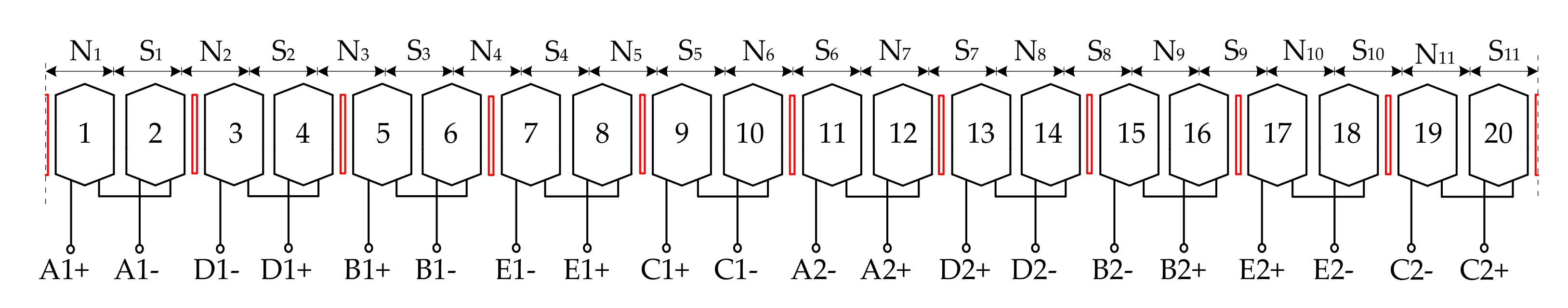
2.1. Five-Phase PMSM Healthy Model

The motor studied in this paper is a new type of five-phase PMSM with no electromagnetic coupling and low thermal coupling between windings and was developed from the traditional five-phase PMSM with 20 slots and 22 poles. The profile diagram and stator winding expansion diagram are shown in Figure 1 and Figure 2, respectively. By adding small teeth and placing an insulation board on both sides of the small teeth, low thermal coupling and no electromagnetic coupling between the windings of each phase can be realized [27]. To observe the situation where there is no electromagnetic coupling between each phase winding after adding the small teeth, the current excitation is only applied to the A2 phase winding, and the magnetic field distribution of the stator is shown in Figure 3. Due to the existence of small teeth, the armature reaction magnetic field has no cross link with other phase windings, which indicates that there is no electromagnetic coupling between each phase winding of the motor. When the ISCF occurs in the winding of a certain phase, the magnetic field generated by the short-circuit current will not generate electromagnetic induction with other windings, which will improve the fault-tolerant control performance when the ISCF occurs.

When the five-phase PMSM is healthy, the phase voltage balance equation matrix can be expressed as

$$u_{5\mathrm{s}}=R{i}_{5\mathrm{s}}+L\frac{\mathrm{d}}{\mathrm{d}t}{i}_{5\mathrm{s}}+e_{5\mathrm{s}}$$

(1)

where R and L are the phase resistance and phase inductance, respectively; $u_{5\mathrm{s}}$, $i_{5\mathrm{s}}$, and $e_{5\mathrm{s}}$ are, respectively, the phase voltage, phase current, and phase permanent magnet reverse EMF matrix:

$$u_{5\mathrm{s}}={\left[\begin{array}{ccccc}{u}_{\mathrm{A}}& u_{\mathrm{B}}& u_{\mathrm{C}}& u_{\mathrm{D}}& u_{\mathrm{E}}\end{array}\right]}^{\mathrm{T}}$$

(2)

$$i_{5\mathrm{s}}={\left[\begin{array}{ccccc}{i}_{\mathrm{A}}& i_{\mathrm{B}}& i_{\mathrm{C}}& i_{\mathrm{D}}& i_{\mathrm{E}}\end{array}\right]}^{\mathrm{T}}$$

(3)

$$e_{5\mathrm{s}}={\left[\begin{array}{ccccc}{e}_{\mathrm{A}}& e_{\mathrm{B}}& e_{\mathrm{C}}& e_{\mathrm{D}}& e_{\mathrm{E}}\end{array}\right]}^{\mathrm{T}}$$

(4)

When the amplitude of the fundamental component of the permanent magnet flux at each pole is ${\Phi }_{\mathrm{m}}$, and the number of turns of each coil is $N_{\mathrm{c}}$, the effective value of the fundamental component of the permanent magnet back EMF in each phase winding can be expressed as

$$E=2\sqrt{2}\omega k_q{k}_y{N}_{\mathrm{c}}{\Phi }_{\mathrm{m}}$$

(5)

where $\omega$ is the fundamental electric angular velocity; and $k_q$ and $k_y$ are the distribution coefficient and short distance coefficient, respectively.

The electromagnetic torque of the five-phase PMSM can be expressed as

$$T_{\mathrm{e}}=\frac{p_{\mathrm{n}}}{\omega }\left(i_{\mathrm{A}}{e}_{\mathrm{A}}+i_{\mathrm{B}}{e}_{\mathrm{B}}+i_{\mathrm{C}}{e}_{\mathrm{C}}+i_{\mathrm{D}}{e}_{\mathrm{D}}+i_{\mathrm{E}}{e}_{\mathrm{E}}\right)$$

(6)

where $p_{\mathrm{n}}$ is pole pairs of the five-phase PMSM.

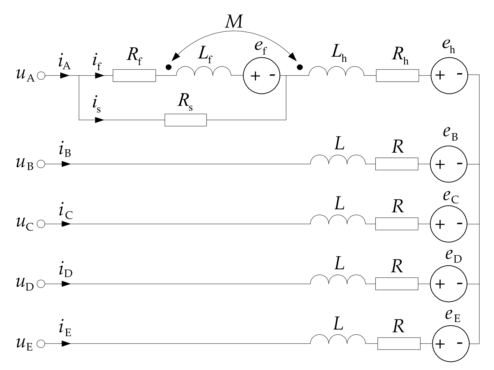
2.2. Five-Phase PMSM Faulty Model

Assuming that the ISCF occurs in phase A, the equivalent circuit diagram of the motor is shown in Figure 4. The reference directions of the voltage, current, and back EMF are given, where $i_{\mathrm{A}}$, $i_{\mathrm{B}}$, $i_{\mathrm{C}}$, $i_{\mathrm{D}}$, and $i_{\mathrm{E}}$ represent the instantaneous value of the stator current of each phase; $u_{\mathrm{A}}$, $u_{\mathrm{B}}$, $u_{\mathrm{C}}$, $u_{\mathrm{D}}$, and $u_{\mathrm{E}}$ represent the instantaneous value of the stator voltage of each phase; $e_{\mathrm{f}}$ represents the permanent magnet back EMF on the short-circuit coil; $e_{\mathrm{h}}$ represents the permanent magnet induced EMF on the remaining healthy coils; $e_{\mathrm{B}}$, $e_{\mathrm{C}}$, $e_{\mathrm{D}}$, and $e_{\mathrm{E}}$ represent the instantaneous value of the back EMF of each healthy phase; R and L represent the resistance and inductance in the healthy phase; $i_{\mathrm{f}}$ represents the current flowing through the short-circuit turns; $i_{\mathrm{s}}$ represents the short-circuit current; $R_{\mathrm{f}}$ and $L_{\mathrm{f}}$ represent the short-circuit coil resistance and inductance, respectively; $R_{\mathrm{h}}$ and $L_{\mathrm{h}}$ represent the resistance and inductance of the remaining healthy coils, respectively; $R_{\mathrm{s}}$ represents the contact resistance; and M represents the mutual inductance between the short-circuit coil and the remaining healthy coil in the same phase.

Each physical quantity in phase A satisfies the following relation when the ISCF occurs:

$$u_{\mathrm{A}}=i_{\mathrm{s}}{R}_{\mathrm{s}}+L_{\mathrm{h}}\frac{\mathrm{d}{i}_{\mathrm{A}}}{\mathrm{d}t}+M\frac{\mathrm{d}{i}_{\mathrm{f}}}{\mathrm{d}t}+i_{\mathrm{A}}{R}_{\mathrm{h}}+e_{\mathrm{h}}$$

(7)

$$i_{\mathrm{s}}{R}_{\mathrm{s}}=i_{\mathrm{f}}{R}_{\mathrm{f}}+L_{\mathrm{f}}\frac{\mathrm{d}{i}_{\mathrm{f}}}{\mathrm{d}t}+M\frac{\mathrm{d}{i}_{\mathrm{A}}}{\mathrm{d}t}+e_{\mathrm{f}}$$

(8)

$$e_{\mathrm{A}}=e_{\mathrm{f}}+e_{\mathrm{h}}$$

(9)

$$i_{\mathrm{A}}=i_{\mathrm{f}}+i_{\mathrm{s}}$$

(10)

The voltage equation for the other four-phase windings is the same as Equation (1). At this point, the electromagnetic torque of the five-phase PMSM can be expressed as

$$T_{\mathrm{e}}=\frac{p_{\mathrm{n}}}{\omega }\left(i_{\mathrm{A}}{e}_{\mathrm{h}}+i_{\mathrm{f}}{e}_{\mathrm{f}}+i_{\mathrm{B}}{e}_{\mathrm{B}}+i_{\mathrm{C}}{e}_{\mathrm{C}}+i_{\mathrm{D}}{e}_{\mathrm{D}}+i_{\mathrm{E}}{e}_{\mathrm{E}}\right)$$

(11)

After substituting Equations (9) and (10) into Equation (11), we obtain

$$T_{\mathrm{e}}=\frac{p_{\mathrm{n}}}{\omega }\left[\left(i_{\mathrm{A}}{e}_{\mathrm{A}}+i_{\mathrm{B}}{e}_{\mathrm{B}}+i_{\mathrm{C}}{e}_{\mathrm{C}}+i_{\mathrm{D}}{e}_{\mathrm{D}}+i_{\mathrm{E}}{e}_{\mathrm{E}}\right)-i_{\mathrm{s}}{e}_{\mathrm{f}}\right]$$

(12)

It can be seen from Equation (12) that the electromagnetic torque includes two terms when the interturn short-circuit fault occurs in phase A. The first term is the same as Equation (6), which is equivalent to the electromagnetic torque jointly generated by the five-phase windings in a healthy motor. The second term is related to the permanent magnet back EMF of short-circuit turns and the magnitude and phase of the current flowing through the contact resistance.

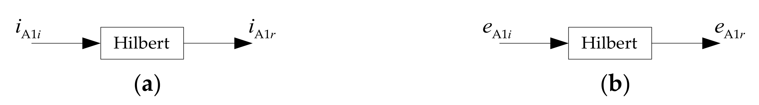
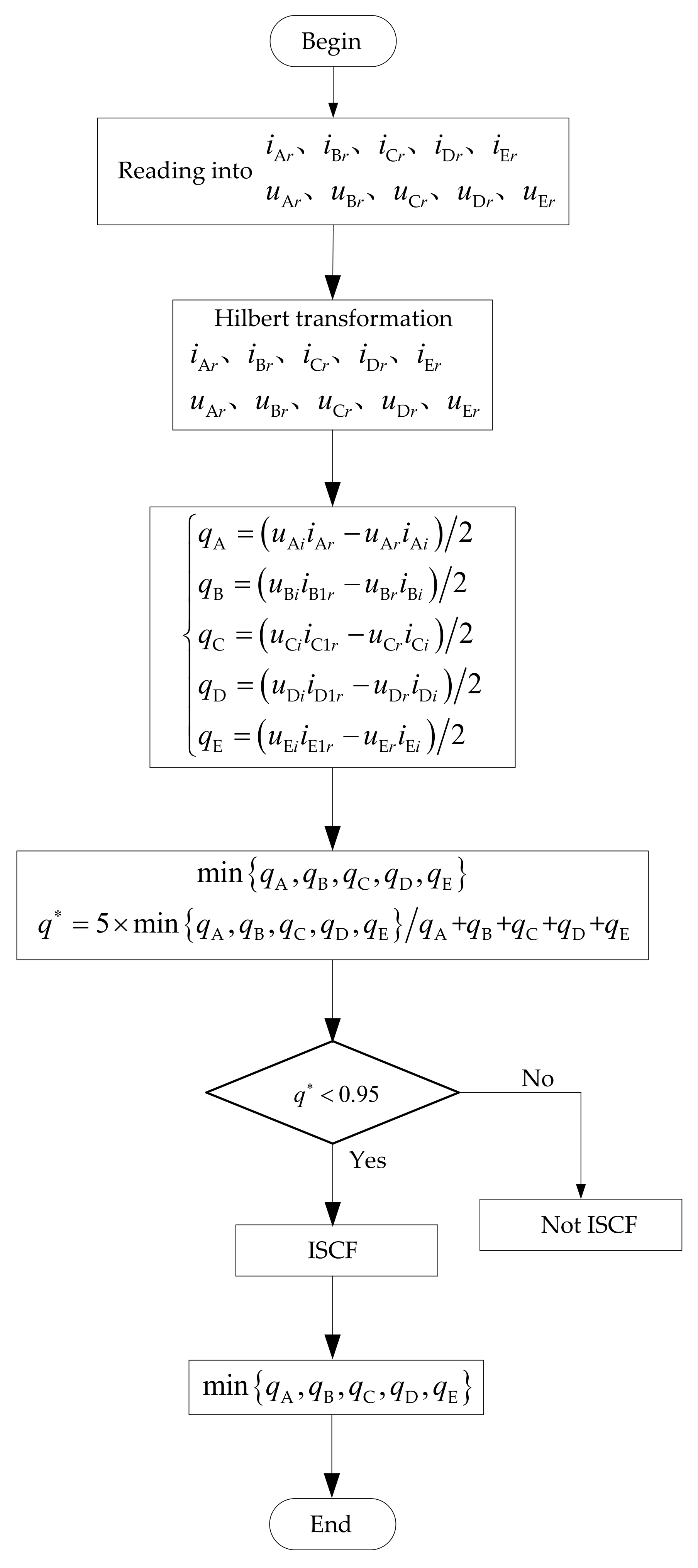
3. Single-Phase Generalized Instantaneous Reactive Power Theory Based on Hilbert Transform

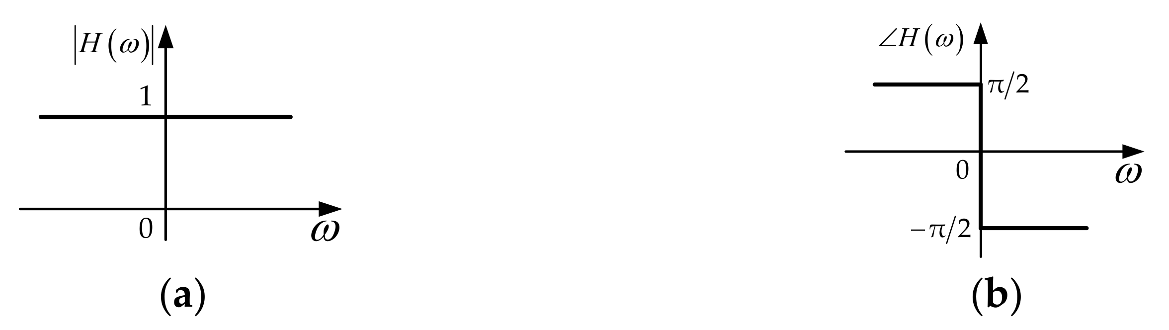
3.1. Principles and Properties of Hilbert Transformation

Hilbert transformation is the theory that defines the relationship between the real and imaginary parts of analytic functions. The analytic function can be expressed as

$$z(t)=x(t)+\mathrm{j}y(t)$$

(13)

where

$$y(t)=h(t)*x(t)$$

(14)

where "*" stands for convolution with time, $x(t)$ can be any function, and $h(t)$ is defined as

$$h(t)=\left\{\begin{array}{cc}0& t\le 0\\ t/\mathsf{\pi }& t>0\end{array}\right.$$

(15)

By using Equation (13)–(15), $y(t)$ is expressed as

$$y(t)={\displaystyle {\int }_0^{t}h(\tau )}x(t-\tau )\mathrm{d}\tau$$

(16)

According to Equation (16), $y(t)$ can be obtained by the integral of the real part’s instantaneous value, and the calculation time can be ignored mathematically. Therefore, from a mathematical point of view, there is no delay time between the real and imaginary parts of the constructed analytic function [28].

The amplitude–frequency and phase–frequency characteristics of the Hilbert transform are shown in Figure 5.

The Hilbert transform is equivalent to a 90° phase shifter, and its essence is that the positive frequency part of the voltage and current will shift after transformation. The real part of the analytic function is the original signal, while the imaginary part is the signal of the phase shift of the original signal of 90° the real part and the imaginary part are mutually orthogonal [29].

The voltage and current signals of phase A are respectively defined as

$$u_{\mathrm{A}}={\displaystyle \sum \sqrt{2}{U}_{\mathrm{A}n}\sin \left(n\omega t-{\phi }_{\mathrm{A}n}^u\right)}$$

(17)

$$i_{\mathrm{A}}={\displaystyle \sum \sqrt{2}{I}_{\mathrm{A}n}\sin \left(n\omega t-{\phi }_{\mathrm{A}n}^i\right)}$$

(18)

where n is the harmonic number; $U_{\mathrm{A}n}$ and $I_{\mathrm{A}n}$ are the effective values of the n-th harmonic voltage and current of phase A, respectively; and ${\phi }_{\mathrm{A}n}^u$ and ${\phi }_{\mathrm{A}n}^i$ are the initial phase angle of the n-th harmonic voltage and current of phase A.

Figure 6 shows the orthogonal signal of phase A obtained by Hilbert transform.

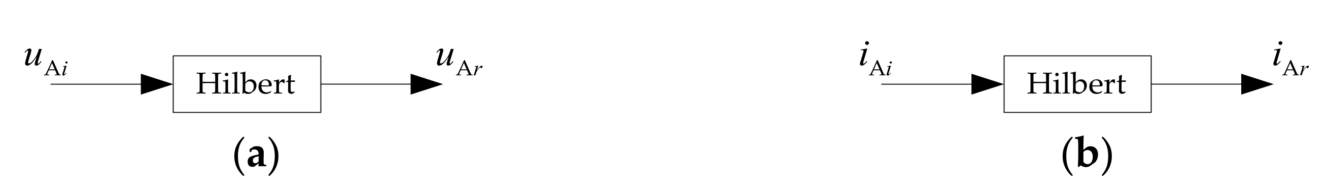
3.2. Principles and Properties of Single-Phase Generalized Instantaneous Reactive Power Theory

The theory of instantaneous reactive power was first proposed by Akagi in 1983 [30]. By transforming the three-phase static coordinate system to a two-phase static system, the three-phase signal was converted into a two-phase orthogonal signal to calculate the instantaneous reactive power of the three-phase system:

$$q=u_{\beta }{i}_{\alpha }-u_{\alpha }{i}_{\beta }=\overline{q}+\tilde{q}$$

(19)

where $\overline{q}$ corresponds to the instantaneous reactive power generated by the interaction of the fundamental wave components in the voltage and current, which is the DC component; and $\tilde{q}$ corresponds to the instantaneous reactive power generated by the interaction of the harmonic components in the voltage and current, which is the AC component.

This theory does not apply to calculating the instantaneous reactive power of a single-phase circuit. However, the voltage and current orthogonal signals constructed by Hilbert transform can be used to calculate the generalized instantaneous reactive power of phase A:

$$q_{\mathrm{A}}=\left(u_{\mathrm{A}i}{i}_{\mathrm{A}}{}_r-u_{\mathrm{A}r}{i}_{\mathrm{A}i}\right)/2$$

(20)

When the five-phase PMSM is healthy and only the fundamental components of phase A are considered, the orthogonal signals of the current and permanent magnet back EMF can be obtained as shown in Figure 7.

The voltage equation can be expressed as

$$\left[\begin{array}{c}{u}_{\mathrm{A}1r}\\ u_{\mathrm{A}1i}\end{array}\right]=R\left[\begin{array}{l}{i}_{\mathrm{A}1r}\\ i_{\mathrm{A}1i}\end{array}\right]+L\frac{\mathrm{d}}{\mathrm{d}t}\left[\begin{array}{c}{i}_{\mathrm{A}1r}\\ i_{\mathrm{A}1i}\end{array}\right]+\left[\begin{array}{l}{e}_{\mathrm{A}1r}\\ e_{\mathrm{A}1i}\end{array}\right]$$

(21)

By substituting Equation (21) into Equation (20), the following can be obtained after calculation and simplification:

$$q_{\mathrm{A}1}=\omega L{I}_{\mathrm{A}1}^2+E_{\mathrm{A}1}{I}_{\mathrm{A}1}\sin \left({\phi }_{\mathrm{A}1}^i-{\phi }_{\mathrm{A}1}^e\right)$$

(22)

where $q_{\mathrm{A}1}$ represents the fundamental wave generalized instantaneous reactive power of phase A, which is obviously a DC value. $E_{\mathrm{A}1}$ is the effective value of the fundamental back EMF of phase A, and ${\phi }_{\mathrm{A}1}^e$ is the initial phase angle of the fundamental back EMF of phase A, which can be determined according to the position between the direct axis of the rotor and the axis of phase A.

Qualitative analysis shows that, when considering the existence of harmonic components, such as the interaction between the fundamental voltage and the third harmonic current or the interaction between the third harmonic voltage and the fundamental current, the second harmonic generalized instantaneous reactive power will be generated. Therefore, $q_{\mathrm{A}}$ can be expressed as

$$q_{\mathrm{A}}={\overline{q}}_{\mathrm{A}}+{\tilde{q}}_{\mathrm{A}}$$

(23)

From the above analysis, it can be seen that when various harmonics are considered, the single-phase generalized instantaneous reactive power theory based on Hilbert transform has the same properties as the three-phase instantaneous reactive power theory proposed by Akagi. In Equation (23), ${\overline{q}}_{\mathrm{A}}$ corresponds to the generalized instantaneous reactive power generated by the interaction of the fundamental wave components in the voltage and current, and ${\tilde{q}}_{\mathrm{A}}$ corresponds to the generalized instantaneous reactive power generated by the interaction of the harmonic components of the voltage and current.

4. Analysis of the Method for Detecting the ISCF

4.1. The Theoretical Analysis

Only the fundamental component is analyzed. When the ISCF occurs in phase A, Equation (8) and Equation (9) are substituted into Equation (7), and then the orthogonal signal of the voltage of phase A can be expressed as

$$\left[\begin{array}{c}{u}_{\mathrm{A}1r}\\ u_{\mathrm{A}1i}\end{array}\right]=R_{\mathrm{f}}\left[\begin{array}{c}{i}_{\mathrm{f}1r}\\ i_{\mathrm{f}1i}\end{array}\right]+\left(L_{\mathrm{h}}+M\right)\frac{\mathrm{d}}{\mathrm{d}t}\left[\begin{array}{c}{i}_{\mathrm{A}1r}\\ i_{\mathrm{A}1i}\end{array}\right]+\left(L_{\mathrm{f}}+M\right)\frac{\mathrm{d}}{\mathrm{d}t}\left[\begin{array}{c}{i}_{\mathrm{f}1r}\\ i_{\mathrm{f}1i}\end{array}\right]+\left[\begin{array}{c}{e}_{\mathrm{A}1r}\\ e_{\mathrm{A}1i}\end{array}\right]$$

(24)

where

$$\left[\begin{array}{c}{i}_{\mathrm{f}1r}\\ i_{\mathrm{f}1i}\end{array}\right]=\left[\begin{array}{c}\sqrt{2}{I}_{\mathrm{f}1}\sin \left(\omega t-{\phi }_{\mathrm{f}1}^i\right)\\ -\sqrt{2}{I}_{\mathrm{f}1}\cos \left(\omega t-{\phi }_{\mathrm{f}1}^i\right)\end{array}\right]$$

(25)

where $I_{\mathrm{f}1}$ and ${\phi }_{\mathrm{f}1}^i$ are the effective value and the initial phase angle of the fundamental current in the short-circuit coil, respectively.

When an ISCF occurs, the generalized instantaneous reactive power of phase A can be expressed as

$$\begin{array}{c}{q}_{\mathrm{A}1}=R_{\mathrm{f}}{I}_{\mathrm{f}1}{I}_{\mathrm{A}1}\sin \left({\phi }_{\mathrm{A}1}^i-{\phi }_{\mathrm{f}1}^i\right)+\omega \left(M+L_{\mathrm{f}}\right)I_{\mathrm{f}1}{I}_{\mathrm{A}1}\cos \left({\phi }_{\mathrm{A}1}^i-{\phi }_{\mathrm{f}1}^i\right)\\ +\omega \left(M+L_{\mathrm{h}}\right)I_{\mathrm{A}1}^2+E_{\mathrm{A}1}{I}_{\mathrm{A}1}\sin \left({\phi }_{\mathrm{A}1}^i-{\phi }_{\mathrm{A}1}^e\right)\end{array}$$

(26)

By calculating the inductance value and resistance value of phase A, when the speed n is equal to 10 r/min, $\omega \left(M+L_{\mathrm{f}}\right)$ is approximately equal to $R_{\mathrm{f}}$. Because the inductive reactance is proportional to the motor speed, when the rotational speed n is greater than 100 r/min, $\omega \left(M+L_{\mathrm{f}}\right)$ is much greater than $R_{\mathrm{f}}$. According to the trigonometric functions, when $\left({\phi }_{\mathrm{A}1}^i-{\phi }_{\mathrm{f}1}^i\right)$ is between $3\mathsf{\pi }/4$ and $3\mathsf{\pi }/2$, and n is greater than 100 r/min, the sum of the first two terms in Equation (26) must be negative. The first two terms are the main factors affecting the change of the generalized instantaneous reactive power, while the latter two terms do not change obviously before and after the ISCF. The generalized instantaneous reactive power expressions of the other healthy phase windings are consistent with Equation (22) before and after the ISCF. Due to the absence of the first two terms in Equation (26), the generalized instantaneous reactive power of the healthy phase windings will not decrease obviously even if the amplitude and phase of the back EMF and the current of the healthy phase windings change after the ISCF occurs. Therefore, by comparing the changes in the generalized instantaneous reactive power of each phase before and after the ISCF with Hilbert transform, it can be determined whether the motor has an ISCF. If the generalized instantaneous reactive power of a certain phase has a certain decrease in amplitude, that phase can be considered the fault phase.

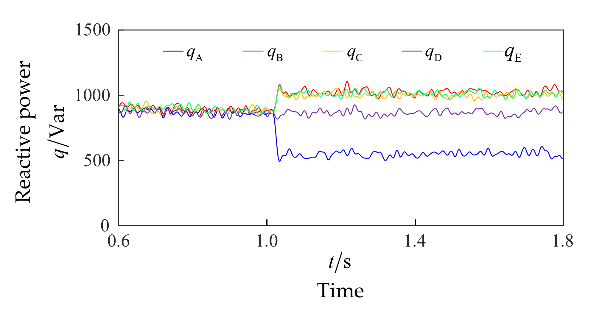
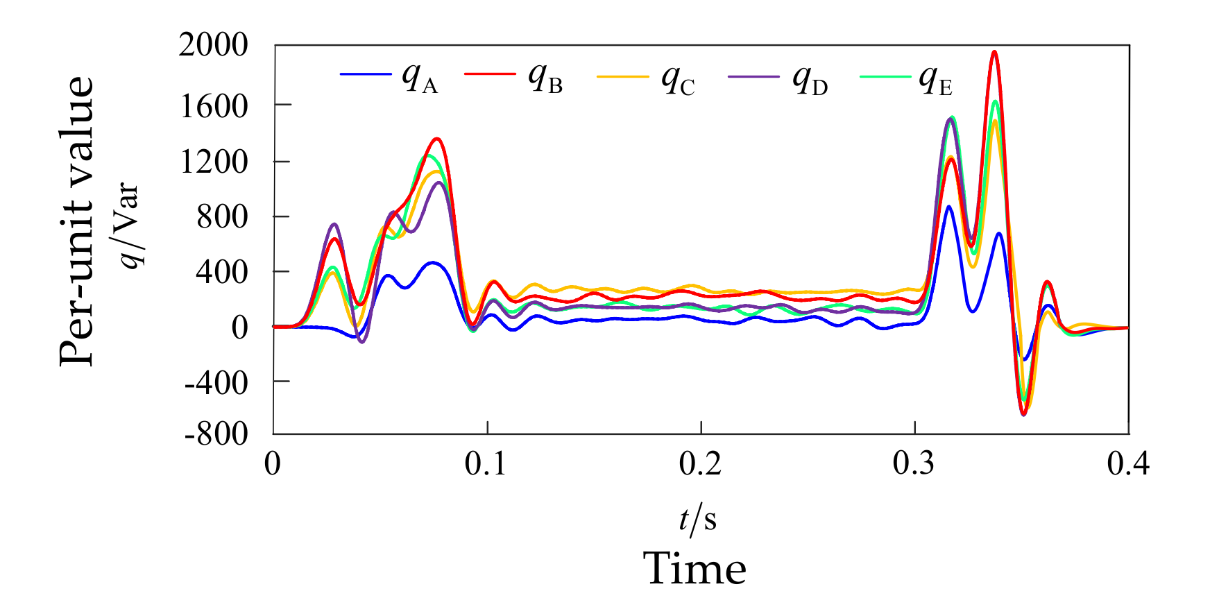
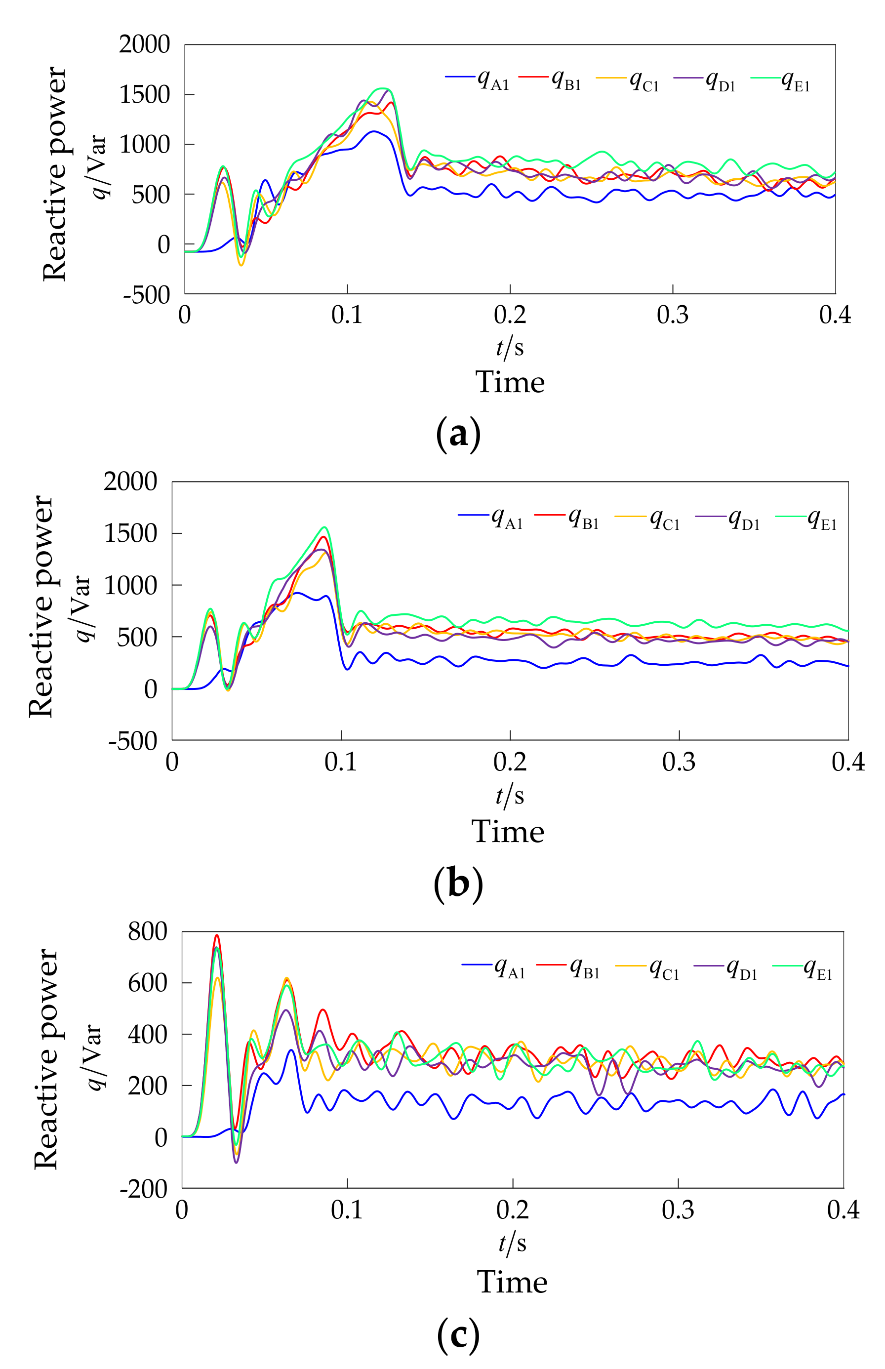
4.2. Simulation Analysis of ISCF Detection under Steady-State Operation

The main parameters of the five-phase PMSM are shown in

Table 1. Parameters of five-phase PMSM.

Parameter	Value
Rated power $P_N$	6.3 kW
Rated speed $n_N$	600 rpm
Rated current $I_N$	22 A
Stator resistance R	0.1638 Ω
Stator inductance L	3.5 mH
1st PM flux linkage ${\psi }_{\mathrm{f}1}$	0.121 Wb
3rd PM flux linkage ${\psi }_{\mathrm{f}3}$	0.0051 Wb
The number of turns per coil $N_{\mathrm{c}}$	25
Pole pair $p_{\mathrm{n}}$	11
Half of small teeth κ	π/180 rad

.

The ratio of the number of short-circuit turns $N_{\mathrm{s}}$ to the total number of turns in a coil $N_{\mathrm{c}}$ is defined as the shorted turn ratio $\zeta =N_{\mathrm{s}}/N_{\mathrm{c}}$, which is strongly related to the severity of the ISCF. The generalized instantaneous reactive power expressions of each phase can be expressed as

$$\left\{\begin{array}{l}{q}_{\mathrm{A}1}=\left(u_{\mathrm{A}1i}{i}_{\mathrm{A}1r}-u_{\mathrm{A}1r}{i}_{\mathrm{A}1i}\right)/2\\ q_{\mathrm{B}1}=\left(u_{\mathrm{B}1i}{i}_{\mathrm{B}1r}-u_{\mathrm{B}1r}{i}_{\mathrm{B}1i}\right)/2\\ q_{\mathrm{C}1}=\left(u_{\mathrm{C}1i}{i}_{\mathrm{C}1r}-u_{\mathrm{C}1r}{i}_{\mathrm{C}1i}\right)/2\\ q_{\mathrm{D}1}=\left(u_{\mathrm{D}1i}{i}_{\mathrm{D}1r}-u_{\mathrm{D}1r}{i}_{\mathrm{D}1i}\right)/2\\ q_{\mathrm{E}1}=\left(u_{\mathrm{E}1i}{i}_{\mathrm{E}1r}-u_{\mathrm{E}1r}{i}_{\mathrm{E}1i}\right)/2\end{array}\right.$$

(27)

The waveform of the generalized instantaneous reactive power of each phase is shown in Figure 6 at $\zeta =0.4$, $T_{\mathrm{L}}=60\mathrm{N}\cdot \mathrm{m}$, and n = 600 r/min, where $T_{\mathrm{L}}$ is the load torque before and after the ISCF occurred in phase A at the time of 1 s. The magnitude of the phase difference $\left({\phi }_{\mathrm{A}1}^i-{\phi }_{\mathrm{f}1}^i\right)$ in (27) is shown in Figure 8.

Figure 9 shows that when the ISCF occurs under this condition, the $\left({\phi }_{\mathrm{A}1}^i-{\phi }_{\mathrm{f}1}^i\right)$ remains between $3\mathsf{\pi }/4$ and $3\mathsf{\pi }/2$. According to Equation (26), compared with other healthy phases, the generalized instantaneous reactive power of phase A decreases significantly. Then, by observing the generalized instantaneous reactive power of each phase, it is possible to detect which phase has the ISCF.

It can be seen from Figure 10 that when the $\zeta$ is fixed, the $\left({\phi }_{\mathrm{A}1}^i-{\phi }_{\mathrm{f}1}^i\right)$ decreases with an increase of the $R_{\mathrm{s}}$, and $\left({\phi }_{\mathrm{A}1}^i-{\phi }_{\mathrm{f}1}^i\right)$ increases with an increase of the $\zeta$ when the $R_{\mathrm{s}}$ is fixed. Moreover, according to the theoretical analysis in the previous section, it can be seen that only when the $\left({\phi }_{\mathrm{A}1}^i-{\phi }_{\mathrm{f}1}^i\right)$ is kept between $3\mathsf{\pi }/4$ and $3\mathsf{\pi }/2$ must the generalized instantaneous reactive power of phase A be reduced. Figure 10a shows that when only one turn of the coil is short-circuited, and the $R_{\mathrm{s}}$ is less than 0.015 Ω, $\left({\phi }_{\mathrm{A}1}^i-{\phi }_{\mathrm{f}1}^i\right)$ will be between $3\mathsf{\pi }/4$ and $3\mathsf{\pi }/2$, and the generalized instantaneous reactive power of phase A will be reduced. According to Figure 10b, when the $N_{\mathrm{s}}$ increases and $\zeta$ is greater than 0.2, $\left({\phi }_{\mathrm{A}1}^i-{\phi }_{\mathrm{f}1}^i\right)$ is always in the range of $3\mathsf{\pi }/4$–$3\mathsf{\pi }/2$. At this time, the generalized instantaneous reactive power of phase A decreases obviously, the ISCF can be detected more accurately, and the fault phase winding can be determined.

To reflect the variation of the generalized instantaneous reactive power of phase A under different short-circuit turns, contact resistance levels, motor speeds, and load torques, the per-unit value of the generalized instantaneous reactive power of phase A is used in the following analysis:

$$q_{\mathrm{A}1}^{\ast }=5q_{\mathrm{A}1}/\left(q_{\mathrm{A}1}+q_{\mathrm{B}1}+q_{\mathrm{C}1}+q_{\mathrm{D}1}+q_{\mathrm{E}1}\right)$$

(28)

where $q_{\mathrm{A}1}^{\ast }$ can represent the reduction of the generalized instantaneous reactive power in phase A. To improve the accuracy of fault detection, the reason for the decrease in the generalized instantaneous reactive power of phase A when it is less than 0.95 is defined as the fault of the interturn short circuit.

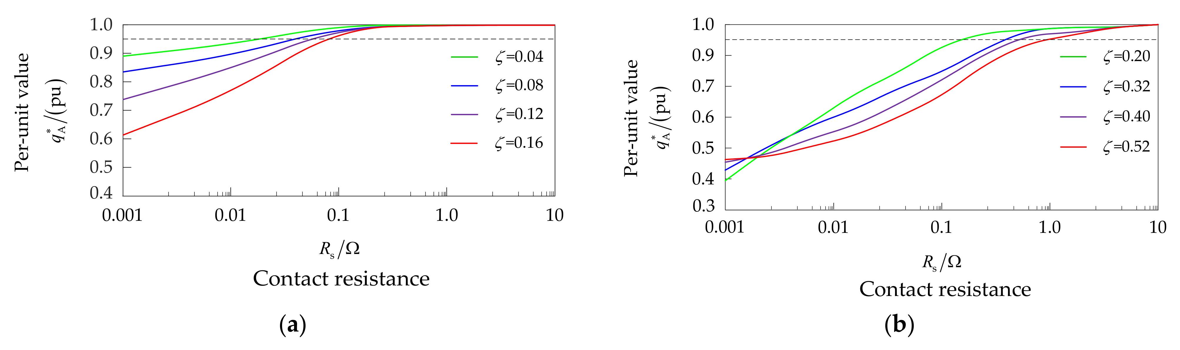
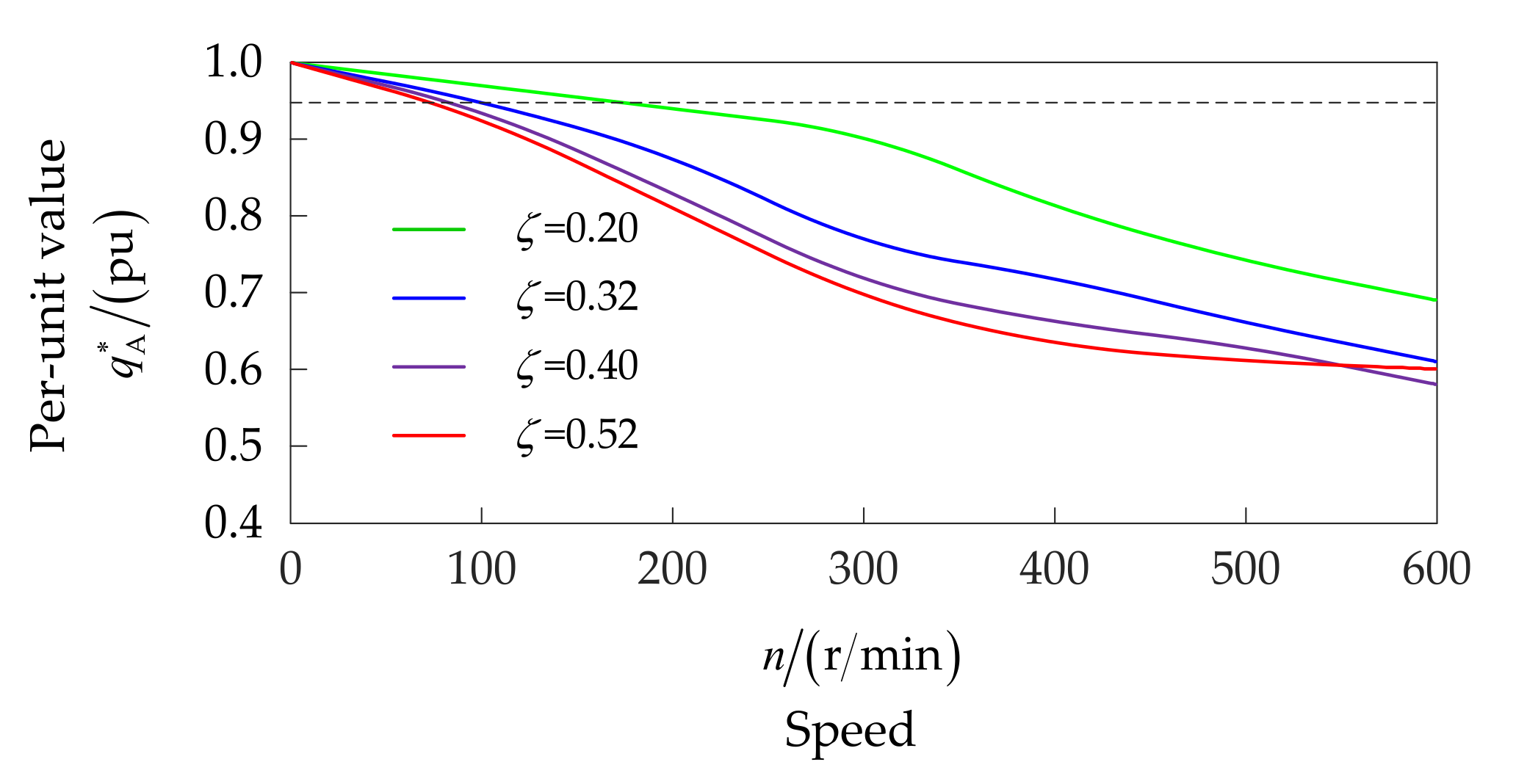
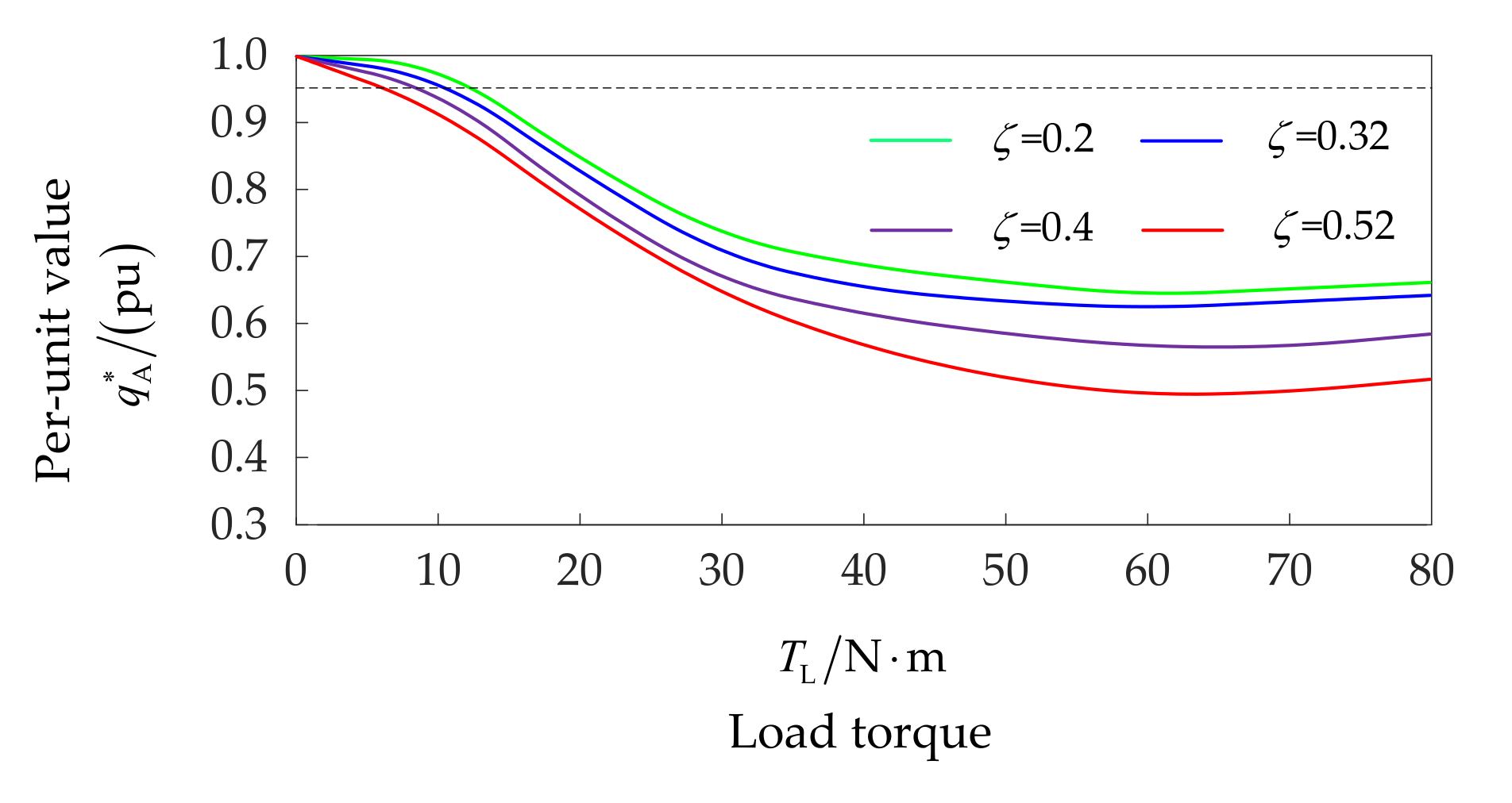
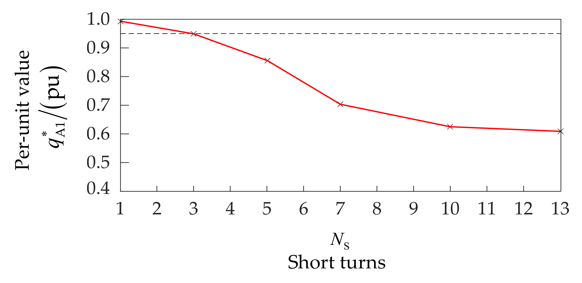
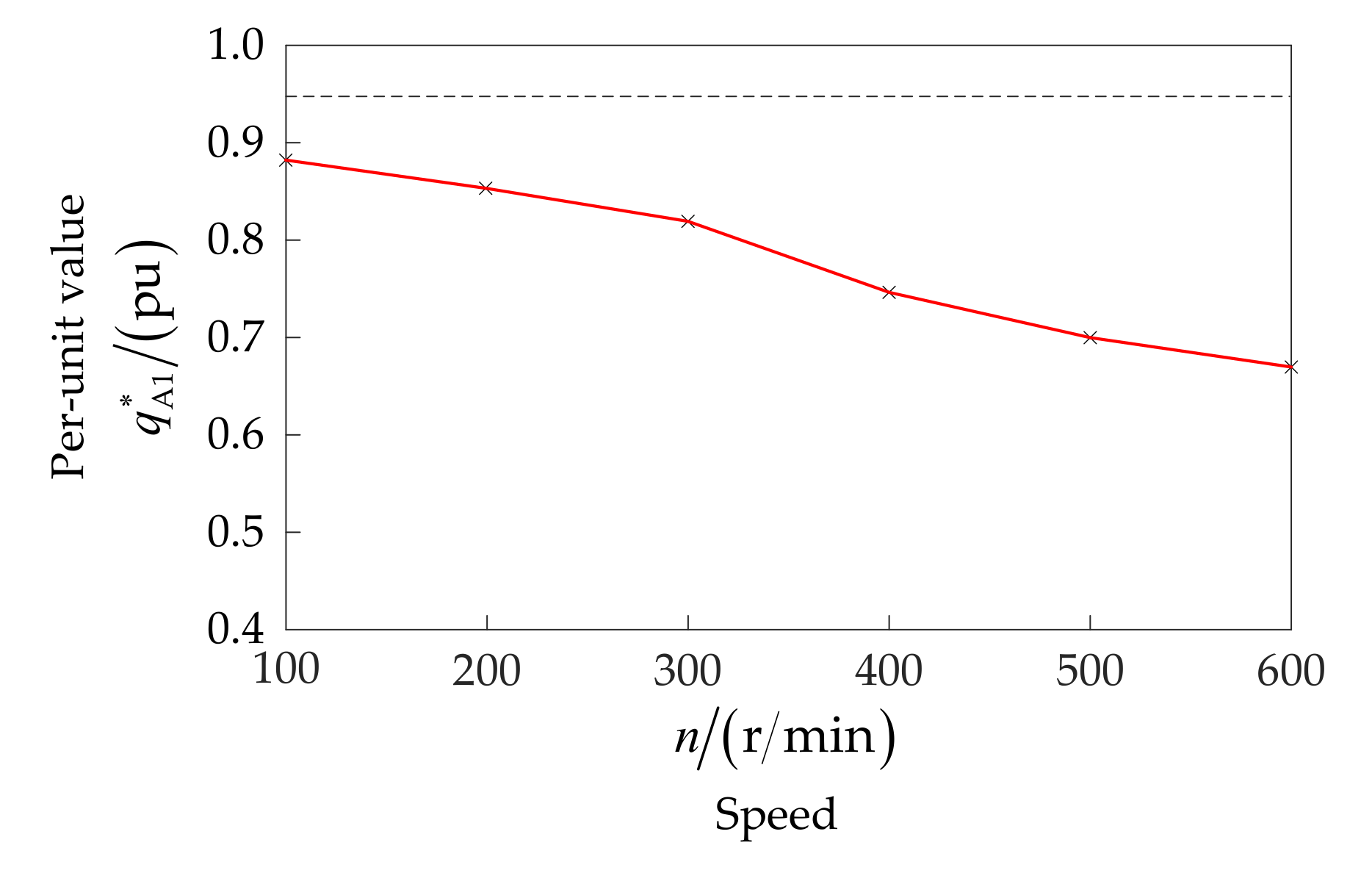
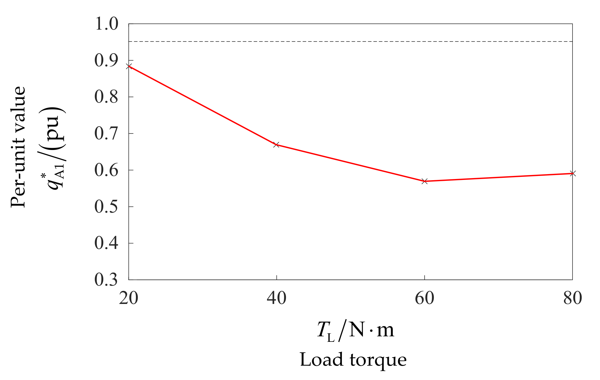
4.3. Analysis of the Influence Factors on the ISCF Detection of a Motor under Steady-State Operation

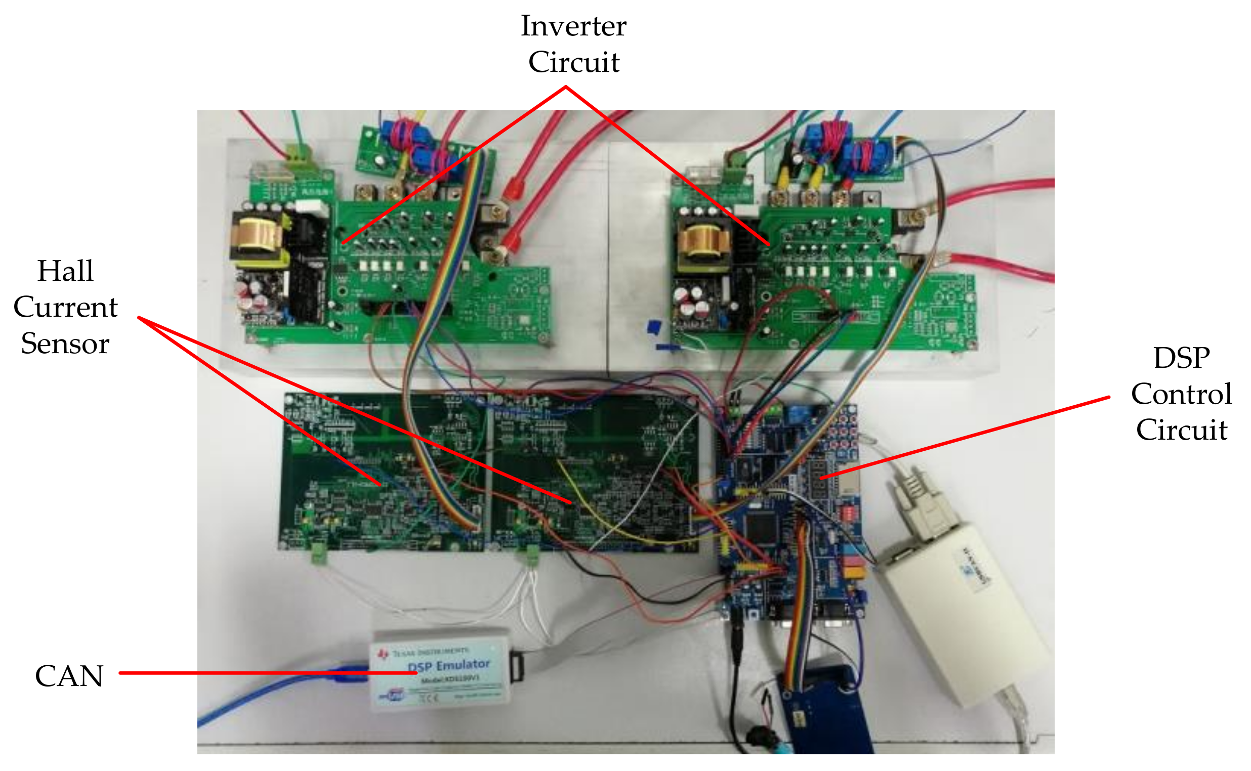
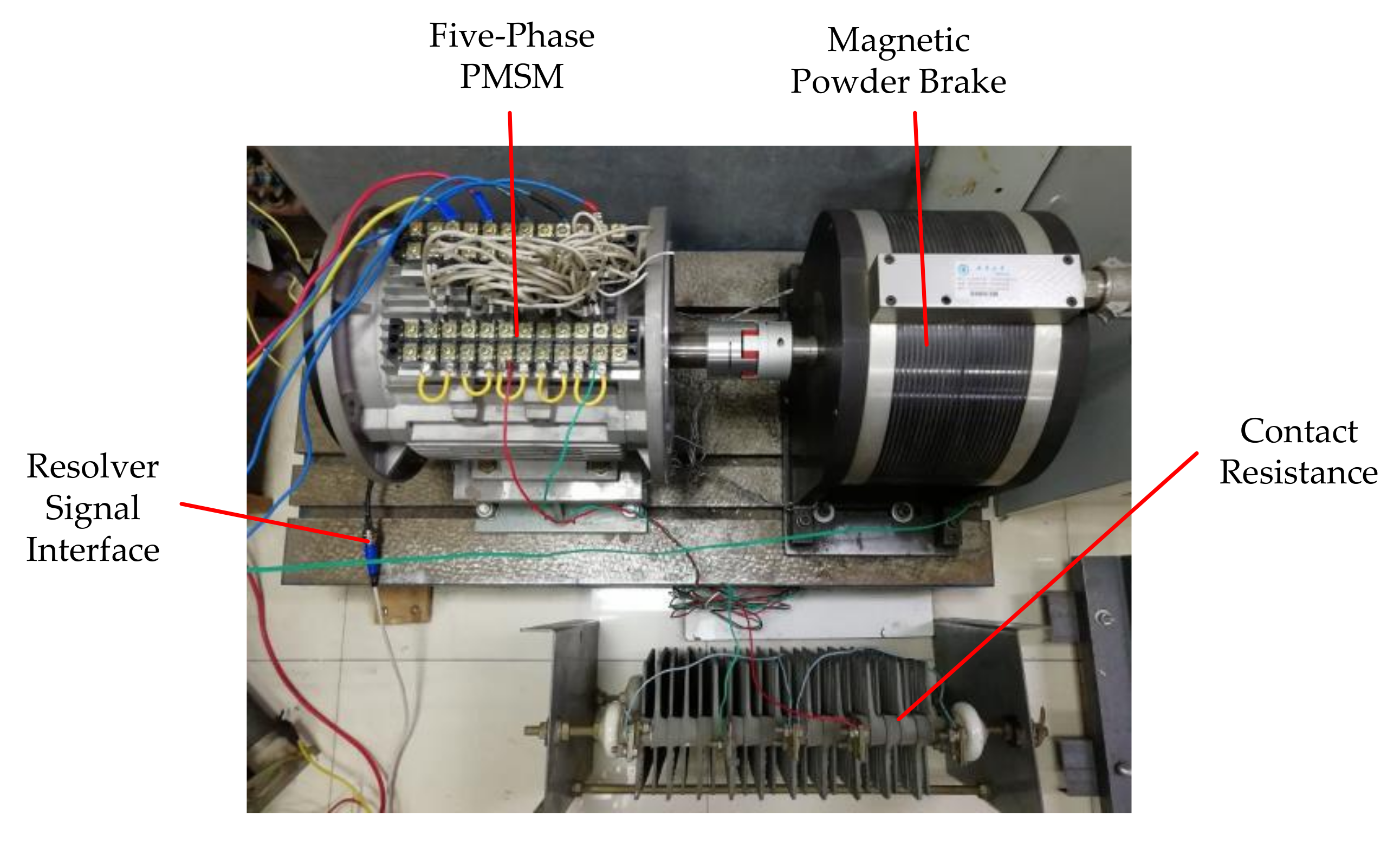
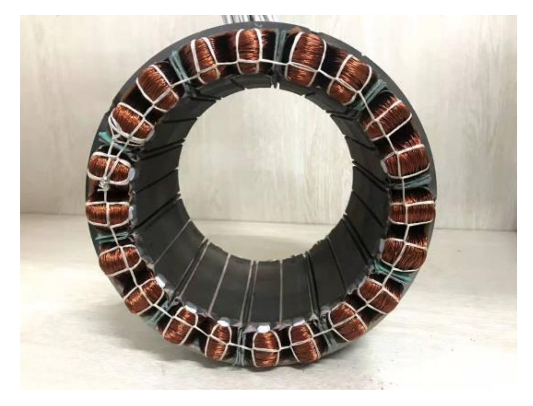
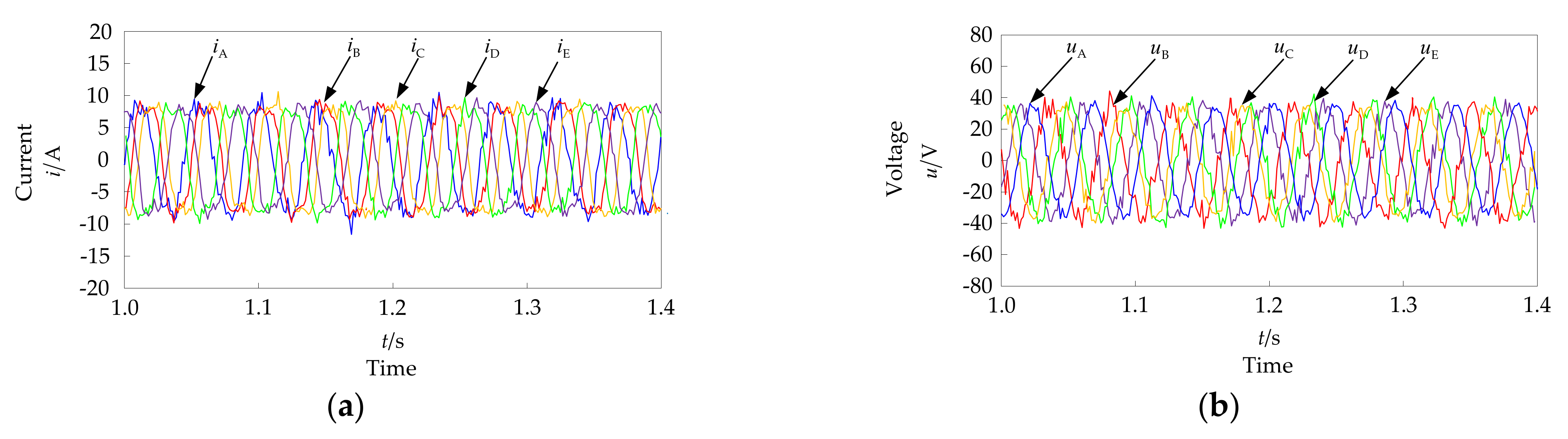
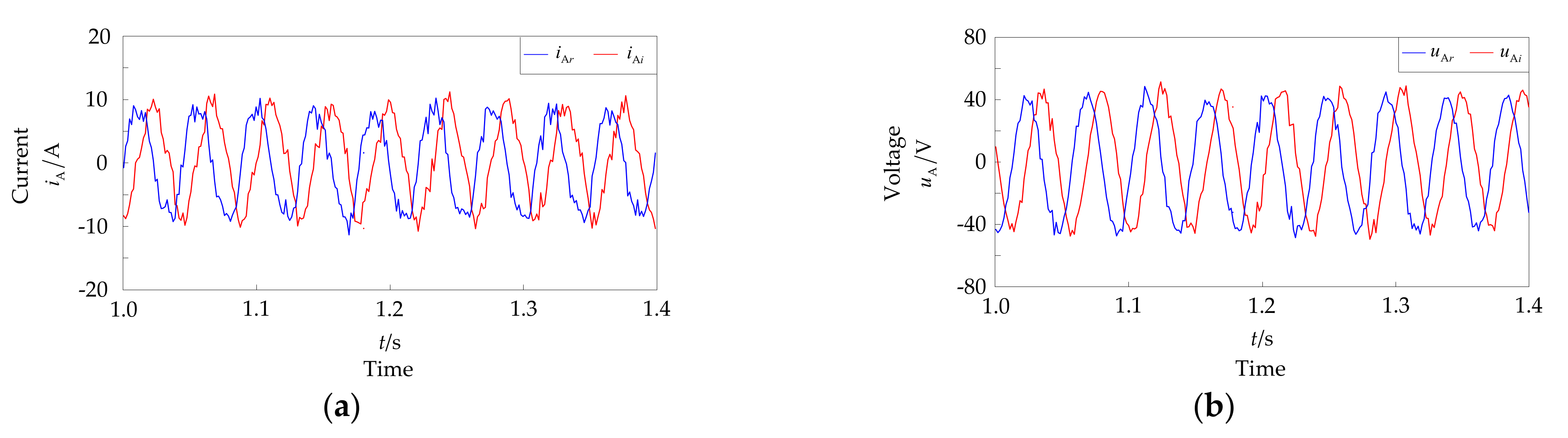
Figure 11, Figure 12, Figure 13 and Figure 14 show the variation of $q_{\mathrm{A}1}^{\ast }$ for contact resistance, short-circuit turns, motor speed, and load torque. Figure 9 shows the variation of $q_{\mathrm{A}1}^{\ast }$ with $N_{\mathrm{s}}$ when the speed and load are constant and $R_{\mathrm{s}}$ is different. It can be seen from Figure 11 that when $R_{\mathrm{s}}$ is constant, with an increase of $N_{\mathrm{s}}$, the value of $q_{\mathrm{A}1}^{\ast }$ becomes smaller, and the detection effect becomes increasingly obvious. When $R_{\mathrm{s}}$ is 0.1 Ω, and $N_{\mathrm{s}}$ is more than 5, $q_{\mathrm{A}1}^{\ast }$ will be less than 0.95. When $R_{\mathrm{s}}$ gradually decreases to 0.01 Ω, the fault can also be detected when the $N_{\mathrm{s}}$ is one turn.

Figure 12 shows the variation of $q_{\mathrm{A}1}^{\ast }$ with $R_{\mathrm{s}}$ when the speed and load are constant, and $N_{\mathrm{s}}$ is different. It can be seen from Figure 12a that $\zeta$ is less than 0.2; only when $R_{\mathrm{s}}$ is less than 0.1 Ω can the value of $q_{\mathrm{A}1}^{\ast }$ be less than 0.95. This is because the number of short-circuit turns is small, and the motor is still close to a healthy state. The inductance and back EMF in fault phase A show little change, so the calculated generalized instantaneous reactive power of phase A also has no obvious change compared to the healthy phase. The detection effect is poor at this time. Figure 12b shows that when $\zeta$ is greater than 0.2, with deterioration of the ISCF, $R_{\mathrm{s}}$ gradually decreases. Here, the short-circuit phenomenon is very obvious.

Figure 13 shows the variation of $q_{\mathrm{A}1}^{\ast }$ with n, where $R_{\mathrm{s}}$ and T_L are constant, and $\zeta$ applies different values. When $\zeta$ is a constant value, the inductive reactance value in the fault phase increases in direct proportion to n and is much larger than $R_{\mathrm{f}}$, so the sum of the first two terms in Equation (28) is negative, and the generalized instantaneous reactive power of phase A decreases significantly compared to the other healthy phases.

Figure 14 shows the variation of $q_{\mathrm{A}1}^{\ast }$ with the T_L, where $R_{\mathrm{s}}$ and n are constant values, and the $\zeta$ applies different values. When the load torque is less than 10 N∙m, $q_{\mathrm{A}1}^{\ast }$ is greater than 0.95 and close to 1. Therefore, the change of the generalized instantaneous reactive power in phase A is very small, and the detection effect is not obvious. As the load torque increases, the load current also increases. According to Equation (28), the reduction of the generalized instantaneous reactive power in phase A is positively correlated with the load current. The $q_{\mathrm{A}1}^{\ast }$ is between 0.45 and 0.95, so the generalized instantaneous reactive power of phase A decreases significantly. At this time, the fault phase can be determined by comparing the difference in the generalized instantaneous reactive power of each phase.

Finally, the ISCF detection in the process of starting the motor, stable operation, and braking is simulated. The simulation conditions are as follows: $\zeta$ is 0.4, $R_{\mathrm{s}}$ is 0.1 Ω, and the given speed is 600 r/min. When the motor runs up to 0.3 s, the given speed command is set to 0 to make the motor brake, and the T_L is always 20 N∙m during the whole operation process. It is thus verified that the ISCF can be detected by comparing the generalized instantaneous reactive power of each phase. Figure 15 shows the variation between the actual speed and given speed. Figure 16 shows the waveform curve of the generalized instantaneous reactive power of each phase. Figure 17 shows the waveform of the generalized instantaneous reactive power of each phase when the motor is started in several different states.

Considering the influence of contact resistance, short-circuit turns, motor speed, and load torque, it can be seen from Figure 11, Figure 12, Figure 13, Figure 14, Figure 15, Figure 16 and Figure 17 that when an ISCF occurs, the generalized instantaneous reactive power of the fault phase will be reduced to a certain extent compared to the other healthy phases, and the fault phase can be determined by using this feature. This method is suitable for both steady and dynamic operations of the motor.

5. Experiments

To verify the feasibility of the online diagnosis method for ISCFs proposed in this paper, the experimental system shown in Figure 18 and Figure 19 was established. Figure 20 shows the stator winding structure of the five-phase PMSM. The load torque here is provided by the magnetic powder brake. The current signal and the voltage signal obtained by inverse transformation of each winding can be transmitted to the host computer through CAN (Controller Area Network) bus data communication. Then, the data can be exported and processed to establish the waveforms.

Figure 21 shows the flow chart of the ISCF of the five-phase PMSM. When the speed in the experiment is 120 r/min, and a five-turn coil around the 12th tooth in phase A is short-circuited, the contact resistance is 0.1 Ω, and the load torque is 20 N·m; the waveforms in the 20 electrical cycles (1.00–1.40 s) in the experiment were then selected. The current signal and the voltage signal obtained by the inverse transformation of each winding are shown in Figure 22. Figure 23 shows the A-phase current signal and voltage signal obtained by sampling and the signal waveform after the Hilbert transform. Figure 24 shows the current and voltage signals after Fourier analysis. As can be seen from Figure 24, compared with the original signal, the amplitude of the signal after the Hilbert transform is almost unchanged.

Through the above method, the current and voltage under different conditions can be obtained; then, the per-unit value of the generalized instantaneous reactive power of phase A can be calculated. Figure 25, Figure 26 and Figure 27 show the variation of $q_{\mathrm{A}1}^{\ast }$ under the experimental conditions, where the contact resistance $R_{\mathrm{s}}=0.1\mathsf{\Omega }$.

6. Conclusions

This paper proposed an ISCF detection method based on single-phase generalized instantaneous reactive power. The main innovation is that this method can not only detect the ISCF but also judge which phase winding the fault occurs in. The orthogonal signals of the current and voltage signals of each phase can be constructed by using a Hilbert transform, and then the generalized instantaneous reactive power of each phase can be calculated. In this paper, the change of the generalized instantaneous reactive power of each phase under different operation states was analyzed in detail. It was found that the generalized instantaneous reactive power of the fault phase is lower than that of the other healthy phases. The proposed ISCF detection method was experimentally verified under different ISCF situations, rotor speeds, and load torques. Finally, the experimental results demonstrated that the proposed method can successfully detect an ISCF.

The early detection of ISCF will be studied in the future. It is hoped that the method proposed in this paper can be improved. Currently, when the number of short-circuit turns is less than five, the ISCF can be detected timely and accurately.

References

1. Ehsani, M.; Gao, Y.; Miller, J.M. Hybrid electric vehicles: Architecture and motor drives. IEEE Proc. 2007, 95, 719–728. [Google Scholar] [CrossRef]
2. Wang, W.; Cheng, M.; Zhang, B.; Zhu, Y.; Ding, S. A fault-tolerant permanent-magnet traction module for subway application. IEEE Trans. Power Electron. 2014, 29, 1646–1658. [Google Scholar] [CrossRef]
3. Jeong, H.; Moon, S.; Kim, S.W. An Early Stage Interturn Fault Diagnosis of PMSMs by Using Negative-Sequence Components. IEEE Trans. Ind. Electron. 2017, 64, 5701–5708. [Google Scholar] [CrossRef]
4. Yang, S.; Hsu, Y.; Chou, P.; Liu, C.; Chen, G.; Li, K. Fault Detection and Tolerant Capability of Parallel-Connected Permanent Magnet Machines Under Stator Turn Fault. IEEE Trans. Ind. Appl. 2018, 54, 4447–4456. [Google Scholar] [CrossRef]
5. Qi, Y.; Zafarani, M.; Gurusamy, V.; Akin, B. Advanced Severity Monitoring of Interturn Short Circuit Faults in PMSMs. IEEE Trans. Transp. Electrif. 2019, 5, 395–404. [Google Scholar] [CrossRef]
6. Qi, Y.; Bostanci, E.; Zafarani, M.; Akin, B. Severity Estimation of Interturn Short Circuit Fault for PMSM. IEEE Trans. Ind. Electron. 2019, 66, 7260–7269. [Google Scholar] [CrossRef]
7. Ge, Y.; Song, B.; Pei, Y.; Mollet, Y.A.B.; Gyselinck, J.J.C. Analytical Expressions of Isolation Indicators for Permanent-Magnet Synchronous Machines Under Stator Short-Circuit Faults. IEEE Trans. Energy Convers. 2019, 34, 984–992. [Google Scholar] [CrossRef]
8. Haddad, R.Z.; Lopez, C.A.; Foster, S.N.; Strangas, E.G. A Voltage-Based Approach for Fault Detection and Separation in Permanent Magnet Synchronous Machines. IEEE Trans. Ind. Appl. 2017, 53, 5305–5314. [Google Scholar] [CrossRef]
9. Moradzadeh, A.; Pourhossein, K.; Mohammadi-Ivatloo, B.; Mohammadi, F. Locating Inter-Turn Faults in Transformer Windings Using Isometric Feature Mapping of Frequency Response Traces. IEEE Trans. Ind. Inform. 2020. [Google Scholar] [CrossRef]
10. Kim, K. Simple Online Fault Detecting Scheme for Short-Circuited Turn in a PMSM Through Current Harmonic Monitoring. IEEE Trans. Ind. Electron. 2011, 58, 2565–2568. [Google Scholar] [CrossRef]
11. Eftekhari, M.; Moallem, M.; Sadri, S.; Hsieh, M. Online Detection of Induction Motor’s Stator Winding Short-Circuit Faults. IEEE Syst. J. 2014, 8, 1272–1282. [Google Scholar] [CrossRef]
12. Zhao, J.; Guan, X.; Li, C.; Mou, Q.; Chen, Z. Comprehensive Evaluation of Inter-Turn Short Circuit Faults in PMSM Used for Electric Vehicles. IEEE Trans. Intell. Transp. Syst. 2020, 1–11. [Google Scholar] [CrossRef]
13. Glowacz, A.; Glowacz, W.; Głowacz, Z. Fault Diagnosis of Three Phase Induction Motor Using Current Signal, MSAF-Ratio15 and Selected Classifiers. Arch. Metall. Mater. 2017, 62, 2413–2419. [Google Scholar] [CrossRef]
14. Qi, Y.; Bostanci, E.; Gurusamy, V.; Akin, B. A Comprehensive Analysis of Short-Circuit Current Behavior in PMSM Interturn Short-Circuit Faults. IEEE Trans. Power Electron. 2018, 33, 10784–10793. [Google Scholar] [CrossRef]
15. Cui, R.; Fan, Y.; Li, C. On-Line Inter-Turn Short-Circuit Fault Diagnosis and Torque Ripple Minimization Control Strategy Based on OW Five-Phase BFTHE-IPM. IEEE Trans. Energy Convers. 2018, 33, 2200–2209. [Google Scholar] [CrossRef]
16. Wu, F.; EL-Refaie, A.M.; Zheng, P. Diagnosis and Remediation of Single-Turn Short Circuit in a Multiphase FSCW PM Machine Based on T-type Equivalent Circuit. IEEE Trans. Ind. Appl. 2020, 56, 158–169. [Google Scholar] [CrossRef]
17. Wu, F.; Tong, C.; Sui, Y. Influence of third harmonic back EMF on modeling and remediation of winding short circuit in a multiphase PM machine with FSCWs. IEEE Trans. Ind. Electron. 2016, 63, 6031–6041. [Google Scholar] [CrossRef]
18. Shichuan, D.; Qingming, W.; Jun, H. Inter-turn fault diagnosis of permanent magnet synchronous machine considering model predictive control. Chin. Soc. Electr. Eng. 2019, 39, 3697–3708. [Google Scholar] [CrossRef]
19. Saitou, M.; Shimizu, T. Generalized theory of instanta-neous active and reactive powers in single-phase circuits based on Hilbert transform. In Proceedings of the 2002 IEEE 33rd Annual IEEE Power Electronics Specialists Conference, Cairns, QLD, Australia, 23–27 June 2002; pp. 1419–1424. [Google Scholar]
20. Lv, K.; Gao, C.; Si, J. Fault coil location of inter-turn short-circuit for direct-drive permanent magnet synchronous motor using knowledge graph. IET Electr. Power Appl. 2020, 14, 1712–1721. [Google Scholar] [CrossRef]
21. Chen, L.; Wang, J.; Sun, Z. Electromagnetic-thermal coupled modelling and analysis of inter-turn short-circuit faults of a permanent magnet alternator. J. Eng. 2019, 2019, 4426–4431. [Google Scholar] [CrossRef]
22. Berzoy, A.; Mohammed, O.A.; Restrepo, J. Analysis of the Impact of Stator Interturn Short-Circuit Faults on Induction Machines Driven by Direct Torque Control. IEEE Trans. Energy Convers. 2018, 33. [Google Scholar] [CrossRef]
23. Sadeghi, R.; Samet, H.; Ghanbari, T. Detection of Stator Short-Circuit Faults in Induction Motors Using the Concept of Instantaneous Frequency. IEEE Trans. Industr. Inform. 2019, 15, 4506–4515. [Google Scholar] [CrossRef]
24. Zhang, J.; Zhan, W.; Ehsani, M. Fault-Tolerant Control of PMSM with Inter-Turn Short-Circuit Fault. IEEE Trans. Energy Convers. 2019, 34, 2267–2275. [Google Scholar] [CrossRef]
25. Sarikhani, A.; Mohammed, O.A. Inter-Turn Fault Detection in PM Synchronous Machines by Physics-Based Back Electromotive Force Estimation. IEEE Trans. Ind. Electron. 2013, 60, 3472–3484. [Google Scholar] [CrossRef]
26. Moon, S.; Jeong, H.; Lee, H.; Kim, S.W. Interturn Short Fault Diagnosis in a PMSM by Voltage and Current Residual Analysis with the Faulty Winding Model. IEEE Trans. Energy Convers. 2018, 33, 190–198. [Google Scholar] [CrossRef]
27. Yiguang, C.; Yuling, P.; Xin, H. Magnetomotive force in permanent magnet synchronous machine with concentrated fractional-slot winding. Trans. China Eletrotech. Soc. 2010, 25, 30–36. [Google Scholar] [CrossRef]
28. Sarkhanloo, M.S.; Ghalledar, D.; Azizian, M.R. Diagnosis of stator winding turn to turn fault of induction motor using space vector pattern based on neural network. In Proceedings of the The 3rd Conference on Thermal Power Plants, Tehran, Iran, 18–19 October 2011; pp. 1–6. [Google Scholar]
29. Yucheng, G.; Wei, Z.; Songling, H. Reactive power definition single-phase circuits based on instantaneous reactive power theory. Electr. Meas. Instrum. 2016, 53, 1–8. [Google Scholar]
30. Akagi, H.; Kanazawa, Y.; Nabae, A. Instantaneous reactive power compensators comprising switching devices without energy storage components. IEEE Trans. Ind. Appl. 2008, 20, 625–630. [Google Scholar] [CrossRef]
Figure 1. Five-phase PMSM profile diagram.
Energies 14 00434 g001
Figure 2. Stator winding expansion diagram.
Energies 14 00434 g002
Figure 3. The magnetic field distribution of the stator.
Energies 14 00434 g003
Figure 4. The equivalent circuit of the five-phase PMSM with ISCF.
Energies 14 00434 g004
Figure 5. Amplitude–frequency and phase–frequency characteristics of Hilbert transform: (a) amplitude–frequency characteristics; (b) phase–frequency characteristics.
Energies 14 00434 g005
Figure 6. The orthogonal signal of phase A obtained by Hilbert transform: (a) Voltage signal of phase A; (b) current signal of phase A.
Energies 14 00434 g006
Figure 7. The orthogonal signals of the current and permanent magnet back EMF: (a) current signal; (b) back EMF signal.
Energies 14 00434 g007
Figure 8. The waveform of generalized instantaneous reactive power.
Energies 14 00434 g008
Figure 9. The magnitude of φ A 1 i φ f 1 i .
Energies 14 00434 g009
Figure 10. Change of φ A 1 i φ f 1 i with ζ and R s : (a) ζ < 0.2 ; (b) ζ > 0.2 .
Energies 14 00434 g010
Figure 11. Change of q A 1 with N s ( n =   600   r / min , T L =   60   N m ).
Energies 14 00434 g011
Figure 12. Change of q A 1 with R s : (a) ζ < 0.2 ; (b) ζ > 0.2 .
Energies 14 00434 g012
Figure 13. Change of q A 1 with n ( R s =   0.1   Ω , T L =   60   N m ).
Energies 14 00434 g013
Figure 14. Change of q A 1 with TL ( R s =   0.1   Ω , n =   600   r / min ).
Energies 14 00434 g014
Figure 15. The variation of the actual speed and given speed.
Energies 14 00434 g015
Figure 16. The generalized instantaneous reactive power of each phase.
Energies 14 00434 g016
Figure 17. The generalized instantaneous reactive power of each phase: (a) ζ = 0.2 , R s =   0.1 , n = 600 r/min, TL = 60 N·m; (b) ζ = 0.2 , R s =   0.1 , n = 600 r/min, TL = 40 N·m; (c) ζ = 0.2 , R s =   0.1 , n = 400 r/min, TL = 60 N·m.
Energies 14 00434 g017
Figure 18. The hardware control system.
Energies 14 00434 g018
Figure 19. Five-phase PMSM experimental platform.
Energies 14 00434 g019
Figure 20. Stator winding structure of the five-phase PMSM.
Energies 14 00434 g020
Figure 21. The flow chart of the ISCF of the five-phase PMSM.
Energies 14 00434 g021
Figure 22. The current signal and the voltage signal obtained by an inverse transformation of each winding: (a) the current signal; (b) the voltage signal obtained by inverse transformation.
Energies 14 00434 g022
Figure 23. The current and voltage signals of phase A and the signals after Hilbert transform: (a) the current signal; (b) the voltage signal.
Energies 14 00434 g023
Figure 24. Fourier analysis of current and voltage signals: (a) the current signal; (b) the voltage signal.
Energies 14 00434 g024
Figure 25. Different short-circuit turns ( T L =   20   N m , n =   120   r / min ).
Energies 14 00434 g025
Figure 26. Different speeds ( T L =   20   N m , ζ =   0.2 ).
Energies 14 00434 g026
Figure 27. Different loads ( ζ =   0.2 , n =   120   r / min ).
Energies 14 00434 g027