Abstract
The reduction in operating and maintenance costs of wind farms is a fundamental element to guarantee the competitiveness and growth of the wind market. Wind turbines are highly dynamic structures prone to wear during their lifetime. Therefore, dynamic monitoring systems represent an excellent option to continuously evaluate their structural conditions. These systems allow early detection of damages, permit a proactive response, minimising downtime, and maximising productivity. In this context, the present paper describes the main results obtained with alternative instrumentation strategies tested in a 2.0 MW onshore wind turbine to reduce the costs of the monitoring equipment and at the same time ensure an adequate accuracy in structural condition evaluation. The data processing strategy encompasses the use of operational modal analysis combined with algorithms that deal with the particularities of operation of the wind turbines to continuously track the main vibration modes. After this automated online identification, the influence of the environmental and operating conditions on the tracked natural frequencies is mitigated, making the detection of abnormal variations of the natural frequencies possible, which might flag the appearance of damage. A database of continuously collected acceleration time series during one year is adopted to test the efficiency of alternative monitoring system layouts in detecting simulated damage scenarios. The tested alternative monitoring layouts present a varying number of sensors, alternative distributions in the wind turbine tower, and different sensor noise levels.
1. Introduction
The correct definition of the Operation and Maintenance strategy is a key aspect for all industry agents involved in wind energy production. Therefore, assessing the integrity of the wind turbines components is a field of study that receives high interest.
The condition-based maintenance strategy relies on the fact that many failures that affect equipment and structures are preceded by specific warnings, conditions or indications that a failure will occur [1,2]. Thus, through the early identification of failures, preventive measures can be taken to prevent severe damage to the monitored components, the spread of damage to other components and, in certain cases, the damage can even be avoided [3,4]. In this way, not only will the repair costs be reduced, but it will also allow for better scheduling of maintenance tasks, which usually translates to reduced wind turbine downtime [5].
In this sense, this paper focuses on the analysis of the results obtained within the scope of a monitoring campaign based on vibrations of a 2 MW onshore wind turbine. It is an extensive and expensive experimental campaign, in which seven force-balance accelerometers with reduced noise levels were installed in three sections along the height of the tower, over more than one year.
The processing of the collected data is based on operational modal analysis techniques [6] and aims to identify the dynamic properties of the structure (natural frequencies, damping ratios and mode shapes) observed in the different operating conditions. In [7], the validity and suitability of the monitoring system and the algorithms implemented for data processing are demonstrated.
In a next step, starting from the same database and the results obtained in the previous work, tools are developed with the objective of identifying structural changes, or damages, in the initial stage of development. The modal properties of the structure are evaluated over the different operating conditions and are monitored over time. Abnormal variations in these properties can thus be detected and the occurrence of structural changes is signalled. The effectiveness of the developed tools was proven through the simulation of four damage scenarios. The theoretical foundations related to the methodology used and the results obtained can be found in [8].
The work presented here serves as a follow-up of previous works. As mentioned, the monitoring system installed is considerably extensive and expensive. In order to reduce investment in the acquisition of monitoring equipment, while ensuring adequate accuracy in detecting damage, the original data are manipulated in order to recreate alternative monitoring solutions, designed considering different budgets. Thus, two different strategies are applied to optimise costs: (1) reduce the number of sensors to be used; (2) use of lower quality sensors. These two strategies can also be combined in order to obtain instrumentation solutions that maximise the benefit/cost ratio. Regarding the first strategy, four alternative layouts are tested for the distribution of a variable number of accelerometers along the height of the tower. The second strategy involves adding noise levels to the recorded acceleration time series. In total, four different noise levels were tested.
The main goals of this study are: (a) to compare the efficiency of the two alternatives adopted to reduce costs (reducing the number of sensors and reducing their quality); (b) define the maximum noise level of the sensors, which allows the obtention of estimates of the modal properties of current wind turbines; (c) define an optimal instrumentation solution (layout and noise level) that can be applied to current wind turbines.
2. Case Study Description
The case study addressed in this work is a Senvion MM82 wind turbine located in Torrão wind farm, in the north of Portugal, which started operating in 2007 (Figure 1a). It is a 2.0 MW wind turbine, with an 82 m diameter up-wind rotor, three pitch controlled blades, variable operating speeds and the hub is 80 m high. The support structure consists of a 76 m high tubular steel tower composed by three segments and a reinforced concrete slab foundation.
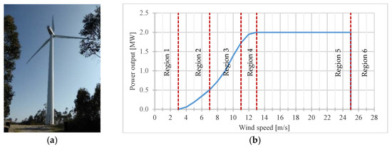
Figure 1.
Senvion MM82-2MW: (a) picture of the wind turbine; (b) wind turbine power curve.
The wind turbine operates for wind speeds between 3 and 25 m/s and achieves the rated power output for wind speeds of about 13 m/s, as seen in the power curve illustrated in (Figure 1b). In the same figure, six operating regions are also illustrated, according to the wind conditions, which determine the action of the wind turbine control mechanisms. The definition of these regions is highly relevant, as they introduce significant variations in the dynamic behaviour of this type of structure. In a simple way, Regions 1 and 6 are associated with nonproduction situations and Regions 2–5 represent different production conditions.
The experimental data used in this study were collected through a vibration-based monitoring system composed of seven uniaxial force-balance accelerometers, distributed in pairs in three sections of the tower (measuring acceleration along two horizontal directions), according to the scheme presented in Figure 2. In the section at a height of two-thirds of the tower height (+48,393 m), a third sensor was added that allows for the characterisation of the torsional movements. However, the pure torsion modes of the tower were not identified.
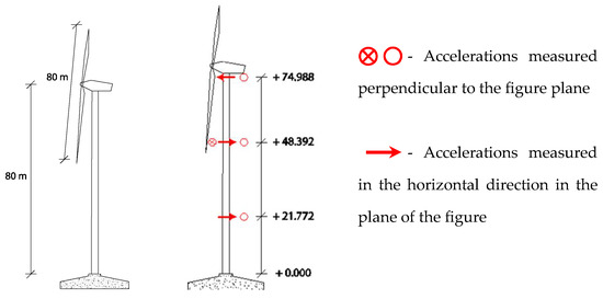
Figure 2.
Position of the accelerometers at three levels of the wind turbine tower.
All instrumentation equipment was located inside the tower. The central acquisition system includes a field computer and a digitiser with a 24-bit analogue-to-digital converter. The digitiser was configured to continuously record 10-min acceleration time series with a sampling frequency of 50 Hz, later decimated to 12.5 Hz.
The collected data were complemented with the information provided by the SCADA system, which continuously characterises the wind turbine’s environmental and operational parameters. Maximum, minimum and average values were recorded for each 10-min interval of several parameters, including wind speed and direction, rotor speed, nacelle orientation, blades pitch angle and outdoor temperature; these are important for the identification of the regions marked in Figure 1b.
In this work, the case study and the monitoring system installed are only briefly described. A detailed description of these aspects and the characterisation of the regions of operation of the wind turbine can be found in [7,8].
3. Data Processing for Vibration-Based Structural Health Monitoring
3.1. Automated Modal Analysis and Damage Detection
As described, damage detection will be carried out based on the identification of abnormal variations in the value of the natural frequencies of the structure. The main goal is to develop a totally autonomous processing methodology, in which the data continuously collected allows the identification of damage situations. This methodology is briefly presented in this section.
The accelerations time series and the parameters provided by the SCADA system are the input data of the processing algorithms. For each 10-min period, the data acquired are processed according to the following four main steps:
- Preprocessing: the recorded acceleration data are decimated (low pass filter and resampling from 50 to 12.5 Hz) to focus the analysis on the frequency range of interest, between 0 and 6 Hz. Then, a coordinate transformation is applied, using the yaw angle provided by the SCADA system, in order to align the signals according to the FA (For-Aft) and SS (Side-Side) directions (horizontal, perpendicular and parallel to the rotor plane, respectively);
- Automated operational modal analysis: the time series of accelerations are processed using three alternative modal identification algorithms: SSI-COV [6], SSI-DATA [9] and p-LSCF [10] combined with postprocessing routines to automate the analysis [11];
- Minimisation of the environmental and operational effects: after the dynamic characterisation of the structure, it is essential to minimise the influence of the operational and environmental effects on the dynamic parameters. In this sense, multivariate linear regression models are applied to reduce their variability. The detailed description of the models implemented in this stage is presented in [8];
- Damage detection: the last step is to identify damage by assessing significant deviations from the reference values of natural frequencies. The implemented procedure is based on the analysis of multivariate control diagrams [12]. This method allows the detection of variations of the various natural frequencies in a single chart.
3.2. Modal Results
With this procedure, several modes of vibration were identified and nine modes were selected to be continuously tracked by the dynamic monitoring system, including bending modes of the tower and rotor. The evolution of nine vibration modes throughout the different operating regimes is presented in a Campbell diagram (Figure 3), where the identified natural frequencies are plotted against the rotor speed. Each mode is identified according to the following nomenclature: order number of the mode followed by the main direction of vibration (FA or SS). If the value of the natural frequency associated with a given mode is clearly dependent on the speed of rotation of the rotor, the graphic sign “*” is added to the name to state that this is driven by the rotor. The configurations of the tracked vibration modes at the tower mode shapes are also represented. The diagram makes it possible to clearly observe the evolution of the value of the natural frequencies of the nine modes of vibration over the operating regimes.
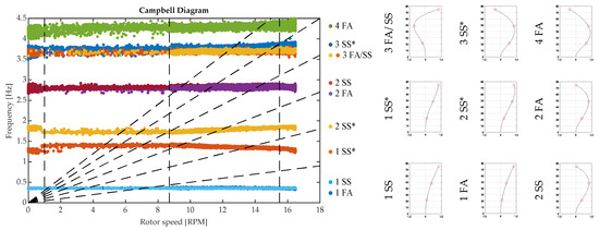
Figure 3.
Campbell diagram with the tracked vibration modes (p-LSCF algorithm) in the left side and corresponding mode shapes in the right side.
Table 1 presents the average values of natural frequencies (), success rates () and the variation coefficient () of the nine vibration modes. Success rates are understood as the ratio between the number of times a particular mode is identified and the total number of files processed (setups). Considering the lower success rates associated with the identification of the last three modes, these will not be considered for damage identification. The selected six modes are also the ones that have the greatest contribution to the dynamic response of the structure.

Table 1.
Statistics related to the results obtained with the three modal identification algorithms.
3.3. Database Characterisation
The installed monitoring system allowed to obtain a database of accelerations during a period of about one year. It is curious to find that only in an insignificant part, around 0.4% of all collected setups, the dynamic parameters of any of the six selected modes were not identified. This shows that the monitoring system is totally adequate for the intended objective and that the data processing and methods implemented are sufficiently robust and are correctly calibrated for the present case study.
However, more relevant than identifying the percentage of data files from which it is possible to extract dynamic parameters from the system, is to identify which files permit the simultaneous identification of the first six modes presented in Table 1. In order to maximise the number of setups to be used in this analysis, we tried to understand which of the tested identification methods had the highest success rate () in the simultaneous identification of the six selected modes. The following results were obtained: ; ; . Despite the fact that the SSI-COV method is the one with the highest success rate (but not as high as pretended), there is a strong interest in increasing the quantity of the available samples. For this purpose, simple arithmetic averages were calculared between the results of the various methods for each of the setups. This allowed the success rate to be increased to 60%, approximately double of what would be achieved with the best method alone. In this way, we sought to take advantage of the complementarity between the methods—that is, extract as much information as possible from each setup. Because, as is easily understood, due to the great variability of operational and environmental conditions, different identification methods are effective in different conditions.
In order to prove the validity of this methodology, statistical analyses were carried out, which involved the study of measures of location, dispersion and distribution of the frequencies obtained with each of the identification algorithms and with the average. These results validated the proposed methodology.
4. Analysis of Alternative Vibration-Based Monitoring Systems
4.1. Strategies: Sensor Layout and Sensor Noise
Two strategies were followed in order to reduce the costs related to monitoring equipment: (1) reducing the number of sensors to be used; (2) using lower quality sensors. These two strategies were combined in order to obtain more economical instrumentation solutions, without compromising the quality of the structural evaluation of wind turbines.
4.1.1. Sensor Layout
The four tested instrumentation layouts are represented in Figure 4. Layout 1 is based on a single pair of sensors located at the top of the tower (+74,988 m). This is an interesting solution as wind turbines are currently equipped with a biaxial accelerometer in this position. The use of this sensor in the evaluation of the structural condition of the tower would represent an important benefit without implying an extra investment.
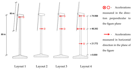
Figure 4.
Alternative sensor layouts.
Although the previous layout has a great advantage in terms of investment in monitoring equipment, it is important to note that due to the reduced amplitude of the modal coordinates associated with the second pair of tower bending modes at this section, it will not be possible to accurately identify these two modes (2 FA and 2 SS). Thus, Layout 2 emerges as an alternative to Layout 1, which optimises the location of the single instrumentation point. In this case, the pair of sensors is approximately two-thirds the height of the tower (height +48,392), which theoretically allows the identification of all important vibration modes.
Layout 3 results from the combination of the previous layouts and is thus based on two biaxial sensors located at the top and two-thirds of the tower height. Layout 4 corresponds to the most complete instrumentation situation, based on seven acceleration recording channels, as described in Section 2. This layout aims to serve as a reference to evaluate the results of the other layouts.
4.1.2. Sensor Quality
The sensors adopted in the monitoring system described in Section 2 are force-balance accelerometers. These are sensors with very low noise levels and with market prices typically exceeding EUR 1500. In order to simulate the time series that would be obtained with low-cost microelectromechanical system (MEMS) sensors, four noise levels were considered: the original noise level of the adopted sensors (N0), and noise levels of sensors rising , and . It is important to note that the higher level of simulated noise is a relatively conservative upper bound, and the intermediate noise levels represent MEMS sensors with prices lower than EUR 500 [13,14].
The new accelerations time series were obtained by adding band-limited white noise time series with varying amplitudes (adjusted according to the simulated noise level) to the measured acceleration time series. This method assumes that the spectral noise of the sensors is constant for the frequency range under analysis, since this is validated by testing accelerometers.
Figure 5 represents the spectra of the time series of accelerations recorded at the top of the tower, considering the defined noise levels for different wind speeds. It was observed that for low wind velocities, all the adopted noise levels surpassed the measured accelerations. However, when the wind velocity reached values of around 2.5 m/s, the first two noise levels were already below the amplitude of the accelerations. The larger noise level was only exceeded by the acceleration signal for relatively high wind velocities.
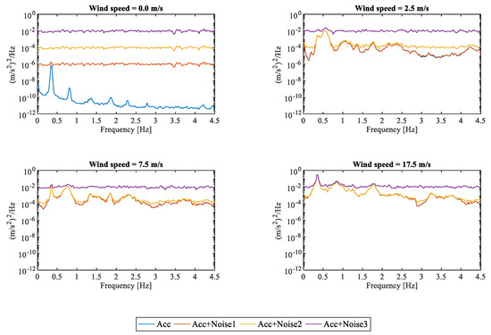
Figure 5.
Power spectra of typical acceleration time series measured at the tower top for varying wind velocities: original signal (Acc) and original signal contaminated with different levels of noise (Acc+Noise1,2,3).
In conclusion, sixteen alternative architecture solutions for dynamic instrumentation of wind turbines are to be tested. Having defined the scenarios to be analysed in the scope of this study, the procedure presented in Section 3.1 was reproduced for each monitoring solution.
4.2. Influence of the Sensor Layout and Noise on the Modal Tracking
In order to make the interpretation of the results more clear, their presentation will be carried out in two stages. In a first phase, we sought to understand the implications of the layouts and noise levels in the identification of the six vibration modes considered for the identification of damage. Then, the performances of each solution were evaluated in relation to the ability to identify damage and the duration of the time interval between the appearance of damage and its detection.
Figure 6 shows the Campbell diagrams associated with some of the adopted monitoring solutions. By comparing the Campbell diagram of Layout 4 N0 (Figure 3) with Layout 4 N2 and N3 (Figure 6a,b), it was observed that as the quality of the sensors decreased (with increased noise), the number of natural frequencies identified for lower rotor speeds (lower excitation levels) were significantly reduced. With noise level N2, it can be seen that the number of identified frequencies for rotor speeds lower than 7 rpm were significantly reduced, but all the modes can still be tracked. For noise level N3, only the second pair of the tower bending modes can be reasonably tracked. For this reason, noise level N3 will not be considered in future analyses.
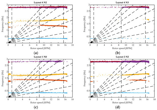
Figure 6.
Campbell diagram with the tracked vibration modes with: (a) Layout 4 N2; (b) Layout 4 N3; (c) Layout 1 N0; (d) Layout 2 N2.
By analysing the diagram associated with Layout 1 and noise level N0 (Figure 6c), it can be seen that and the tracking of the second pair of support structure bending modes was less efficient (lower number of points), especially for a lower rpm. The reduced modal ordinate of these vibration modes at the top of the tower explains this limitation. For this reason, in this layout these two vibration modes will not be considered in the evaluation of the structural condition (only the modes 1 FA, 1 SS, 1 SS*, and 2 SS* will be considered).
The diagram corresponding to Layout 2 with noise level N2 (Figure 6d) shows that even using a single poor quality sensor it is possible to obtain a Campbell diagram with reasonable quality.
This qualitative analysis covering different operation conditions is complemented by the results presented in Figure 7. In this bar plot, the success identification rate (“number of times a mode is identified”/”number of processed setups”) obtained with the alternative layouts and noise levels for Layout 4 is quantified.
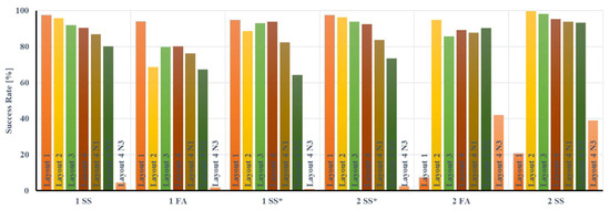
Figure 7.
Success rate in percentage obtained with Layouts 1–4 and noise level for Layout 4 from N0 to N3 (Layouts 1 and 2, MAC limit of 0.5; Layouts 3 and 4N1 to 4N3, MAC limit of 0.8).
For modes 1 SS, 1 FA, 1 SS* and 2 SS* the success rate decreases with the noise level increase, with the reduction being quite extreme for noise level N3. For the second bending mode of tower 2FA, a small increase in the success rate with the increase in noise was observed. This can be explained by the fact that it is the only mode significantly contributing in the response above the noise level; the identification algorithm is just dedicated to this mode.
Finally, Layouts 3 and 4 show very similar success identification rates. For some modes, the success rates obtained with Layouts 1, 2 or 3 are higher than those obtained with the original layout, which indicates that more sensors at the tower may not improve the quality of the results—in particular, the sensor at elevation +21,772 m does not have a significant advantage.
5. Performance Evaluation of Alternative Monitoring Strategies
5.1. Criteria for Performance Evaluation
As mentioned in Section 3.1, multivariate control charts were implemented to flag abnormal variation of the natural frequencies. This consists of a simple statistical tool in which several variables, the natural frequency values of several modes in the present case, are assessed with the statistical test T2 [15].
This procedure is represented schematically in Figure 8. After a training period (Period 1), in which it is assumed that the structure is healthy, it is possible to establish an upper control limit (UCL) to classify an observation as not damaged (considering that 95% of the values from this period are within the safety region). Then, each new observation is assessed with regard to this reference; if the T2 value is greater than this limit, it is assumed that an abnormal event occurred. This is probably motivated by the appearance of damage. A more detailed description of this tool can be found in [12].
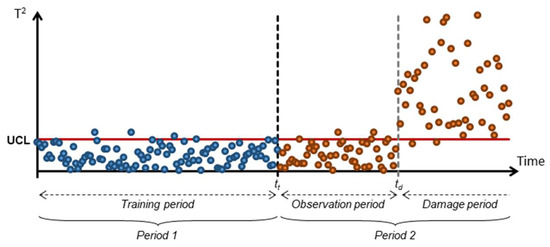
Figure 8.
Procedure implemented to identify abnormal deviations of the natural frequency values.
To obtain more explicit plots with lower scatter, each point of the control chart was calculated from 36 datasets (equivalent to 6 h of data). Only the points associated with Period 2 will be represented in the next section and it was thought that the damage occurred in the middle of Period 2 ().
The evaluation of the performance of the alternative monitoring solutions from the visual analysis of the control charts is possible. However, it is essential to define quantitative criteria that allow a more objective evaluation. Thus, four parameters were established:
- Total number of points on the control chart: this is directly related to the success rates of identification of the selected vibration modes. A greater number of points means a greater number of times that the structure is “examined”, considering the same monitoring period.
- Percentage of outliers in the damage period () computed as:where and are the number of outliers and the number of control points observed in the damaged period, respectively. Thus, should be maximised and its optimal value is 1.
- The indicator quantifies the variation of the T2 index between the scenario without damage and a given damage scenario, and is given by:Thus, higher values of indicate a clearer variation of T2 compared to normal conditions, corresponding to a greater capacity of the layout considered to detect a structural change.
- The time interval between the occurrence of the damage and the moment when the alert is issued. In fact, quantifying response times is not simple and requires criteria to be established. Considering a real case of continuous monitoring of a wind generator, emitting an alarm signal whenever the natural frequencies present a variation greater than the pre-established limit (point of the control graph above the control limit) would not be feasible given the amount of false alarms that would be issued. So, the difficulty lies in defining an automatic and robust enough method that, based on the analysis of the control graphs, detects the structural change with a high degree of assertiveness.
Since in the present work it is only intended to compare the proposed instrumentation solutions, a simple and easy criterion to raise an alarm was adopted. Thus, it was assumed that an anomaly is identified when at least four points on the control chart, in intervals of eight consecutive points, are above the limit. Note that each point corresponds to the observation of 36 data files with a duration of 10 min each. In a perfect monitoring system, each point would correspond to 6 h of observation of the structure. In conclusion, assuming that the monitoring of the wind turbine does not present data flaws and the success rates in identifying the modes are 100%, the hypothesis that the structure presents anomalies is considered valid when, with intervals of 48 h (8 points, 2 days), at least half of the observations are considered anomalous.
5.2. Damage Scenarios
In order to test the capability of each monitoring solution to spot the appearance of damage at an early stage, three damage scenarios were simulated:
- D1: Scour problems at the foundation of an offshore monopile wind turbine;
- D2: Foundation problems in onshore wind turbines;
- D3: Damage in the rotor blades.
The detailed description of the procedures used and the three damage scenarios that are defined here can be found in [8,16]. In the following paragraphs, only a brief description of these same scenarios is presented.
The present case study is an onshore wind turbine and damage scenario D1 is associated with scour problems at the foundation of a monopole offshore wind turbine. However, since the natural frequencies of the case study under analysis present values that are similar to the ones observed on offshore monopile wind turbines [11], this analysis is assumed to be valid. A scour depth of about 0.075 times the base diameter of the monopile was simulated. According to references [17,18], this damage motivates the frequency variations presented in Table 2. This damage has more impact on the second pair of the tower bending modes.
Table 2.
Variation of the natural frequencies associated with tested damage scenarios [%].
Damage scenario D2 can be motivated by problems in the connection between the steel tower and the concrete foundation of onshore wind turbines. It simulates frequency variations in the tower bending modes that are five times smaller than the ones observed in the experimental study reported in [19]. This damage has more impact on the first pair of the tower bending modes.
The last damage scenario (D3) simulates a blade damage. The wind turbine under analysis was modelled in the HAWC2 software [20] to quantify the impact of structural damage at the blades on the natural frequencies 1 SS* and 2 SS*. The blades’ stiffnesses decreased by 15% over a length of 2 m (5% of the total length of the blade) at one-third of the blade length from the blade root. These stiffness reductions motivated the variations of the blades’ frequencies quantified in Table 2.
The representativeness of the simulated damages may be criticised, but the main goal was to show the ability of alternative monitoring layouts to spot very small frequency variations, as the ones presented in Table 2 (all values lower than 1%).
Finally, in order to make data processing less complex and to facilitate the analysis and interpretation of results, certain simplifications were adopted. On the one hand, it was considered that the damage occurs in the middle of Period 2, with the values of natural frequencies being reduced according to the percentages shown in the previous table. On the other hand, it was considered that the damage to the structure occurs instantaneously, disregarding the fact that the magnitude of the damage may increase over time. In the scenario of a growing damage, it would be identified as soon as the simulated intensity is reached.
5.3. Results
In Figure 9, the control diagrams for Layouts 1–4 are represented, considering the noise levels N0, N1 and N2. These diagrams were obtained for the undamaged situation of the structure and for the damage scenarios previously defined as D1, D2 and D3.
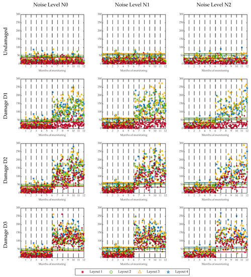
Figure 9.
T2 control charts corresponding to Layouts 1–4 and for noise levels, N0, N1 and N2, considering a scenario undamaged and three damage scenarios, D1, D2 and D3 (the horizontal lines represent the upper control limit (UCL) of each solution).
The analysis of the figure shows that damage scenarios D2 and D3 were identified by all the monitoring solutions under analysis, since after the introduction of the damage most of the points were above the control limit. However, for Layout 1, D1 damage scenario related to erosion problems in the foundation of offshore wind turbines, was not properly detected. As can be seen from the analysis of Table 2, this scenario has more impact on the second pair of tower bending moments and these are not well identified with this instrumentation solution. However, as described in [16], by increasing the variation of the frequency values of the first pair of bending modes by about 2.5 times (to approximately 0.50%) (values associated with still acceptable scour), Layout 1 was able to detect this damage scenario.
5.3.1. Total Number of Points on the Control Chart
The reduction in the quality and number of sensors might be associated with a reduction in the density of points in the control charts, as a result of the reduction in the success rates in the identification of all vibration modes under analysis. This is analysed in Figure 10, which represents the total number of points in the control charts for each monitoring solution.
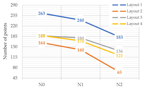
Figure 10.
Number of points of the T2 control charts.
As would be expected, for the same layout, the use of lower quality sensors translates into a reduction in the number of points. This reduction is more pronounced for layouts with only one measurement level (Layouts 1 and 2).
The effect of the reduction in the number of sensors is not so obvious. Layout 2 with only one biaxial sensor is the one with the lowest dot density. Oppositely, Layout 1 is the one with the highest density, although it also has a single measurement level. This is explained by the fact that in its analysis only four of the six main vibration modes are considered, as justified in Section 4.2, and by the high success rates in the identification of these same four modes, as can be seen in Figure 7.
Layouts 3 and 4 present very similar behaviours. It should be noted that for the noise level N0, the difference between them is minimal (Layout 3: 187 points and Layout 4: 188 points). This confirms that the use of an extra measurement level at one-third of the height tower (Layout 4) does not translate into a significant advantage, and for higher noise levels it even translates into a disadvantage. This is justified by the lowest measurement level being located in a position of the structure with reduced vibration levels. When using lower quality sensors (noise level N1 and N2), this measurement level only introduces noise into the system.
5.3.2. Percentage of Outliers in the Damage Period
The relative frequency of outliers in the damage period for the analysed solutions is represented in Figure 11 for each of the damage scenarios. In general, these results confirm the suitability of the proposed instrumentation solutions in detecting the simulated damage scenarios, with the expectation of Layout 1 for damage scenario D1 (values out of the scale adopted for Figure 11a).
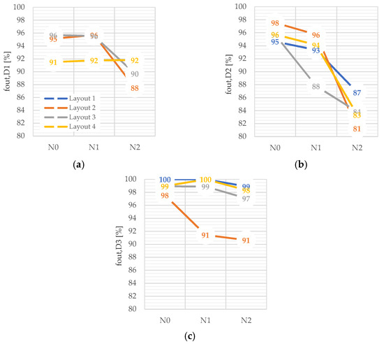
Figure 11.
Relative frequency of outliers: (a) for damage D1; (b) for damage D2; (c) for damage D3.
For damage scenario D1, Layout 4 appears to be insensitive to the reduction in the quality of the sensors. This behaviour is justified by the success rates presented in Figure 7, where it is shown that for Layout 4 there are no changes in the success rates in the identification of the second pair of tower bending modes with the addition of noise. Still, Layouts 2 and 3 exhibit similar behaviours to each other and even show better performances than Layout 4 for noise levels N0 and N1, which indicates that, for the same noise level of the sensors, it is preferable to use a limited and carefully positioned number of sensors, rather than a large number of sensors.
Now considering the D2 damage scenario, it is possible to understand the loss of precision in the control diagrams with the decrease in the quality of the sensors. For the noise level N0, all solutions have very high values (greater than 95%) while for the noise level N2, the results are significantly degraded with values below 90%.
Finally, for damage scenario D3, the majority of the solutions exhibit high performances with values greater than 97%. The only exceptions are Layouts 2 N1 and Layout 2 N2, which still exhibit good performances.
5.3.3. Variation of the T2 Index between Damage and Undamaged Scenarios
The index was determined for each solution using Equation (2). The results obtained for each damage scenario are shown in Figure 12.
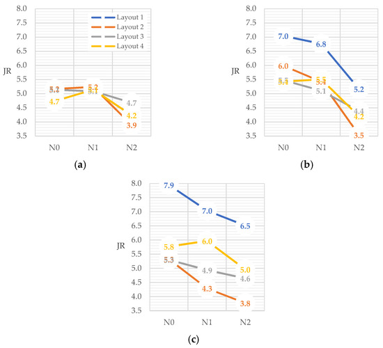
Figure 12.
Performance indicator : (a) damage scenario D1; (b) damage scenario D2; (c) damage scenario D3.
The values obtained for the index for the different solutions once again show a good performance in terms of the identification of structural changes. Since the various solutions are being tested in the identification of slight damage and at an early stage, the fact that in all cases is a very positive indicator.
For the D1 scenario, all solutions present a very similar behaviour to each other and show little influence of the sensor noise levels.
In scenario D2, it turns out that solutions based on Layout 1 have a better performance than the other solutions. Again, this behaviour can be justified on the basis that for Layout 1 only four of the six vibration modes are being used. The rest of the layouts once again show a similar behaviour along the increasing noise levels, with reductions in the index.
Considering the D3 damage scenario, the same conclusions can be drawn for solutions based on Layout 1. For the remaining layouts, there is a clear distinction in their performance. Layout 4 is the one with the second highest values of , while Layout 2 is the one with the lowest values.
5.3.4. Time for Damage Identification
The response times of the various solutions were calculated using the criteria defined in Section 5.1, being the results presented in Figure 13. The response times obtained for most of the instrumentation architectures covered in this work are quite satisfactory. It is possible to identify the presence of damage in less than 7 days, in some cases just 3 days. In fact, since structural changes of very small amplitude are being considered, the possibility of detecting them in less than a week is a very interesting result.
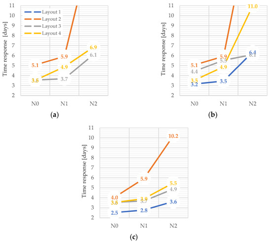
Figure 13.
The response time of optimised monitoring strategies: (a) damage scenario D1; (b) damage scenario D2; (c) damage scenario D3.
The analysis of these figures allows reaching conclusions very similar to those that have already been mentioned during the discussion of the results. As expected, the reduction in sensor quality implies an increase in response times for all systems, with this variation being more pronounced for Layout 2. In all damage scenarios, Layout 2 is the one with the greatest response times. Layout 1 is the one that allows D2 and D3 damage to be detected more quickly. Once again, it is verified that Layouts 3 and 4 present a very similar behaviour, taking advantage of Layout 3 for higher noise levels (N2 and N3).
The minimum response times obtained were 3.5 days for the D1 damage scenario with Layout 4 N0, while for D2 and D3 damage times of 3.2 and 2.5 days were obtained, respectively, using Layout 1 N0. These are very promising results considering the magnitude of the damage considered. These results prove the effectiveness and the importance of the application of vibration monitoring systems in wind generators in order to identify structural changes.
At the opposite extreme, the maximum response times are for Layout 2 N2, with durations of 17.9, 20.4 and 10.2 days for damage scenarios D1, D2 and D3, respectively. Despite being values 4 to 6 times higher than the minimum values, this is not a totally inappropriate solution. Bearing in mind that this solution only requires a low-cost biaxial sensor of the MEM type and that damage of very small amplitude is being considered.
5.3.5. Final Considerations
In Table 3, all the obtained results are summarised, together with a column with indicative costs for the sensors adopted in each layout and a final evaluation. It is important to highlight that the costs are indicative and only include the sensors, being the final cost dependent on the adopted acquisition system and cables or wireless devices. However, their final costs will be approximately proportional to the presented values. So, in the comparison of alternative solutions, ratios between prices should be analysed instead of absolute values. The prices of force-balance sensors (N0) have been less stable over time, whereas, for the MEMS sensors (N1, N2, and N3) a price decrease and quality improvement has been observed.
Table 3.
Comparison of the analysed instrumentation solutions.
One of the objectives of this work was the definition of an optimal combination of layout and noise level of the sensors in order to conceive a monitoring system sufficiently accurate to detect structural changes of the most common wind turbines. However, as it was possible to perceive throughout the results discussion and with the summary in Table 3, there is no one solution that brings together all the advantages and stands out noticeably before the others. In fact, as expected, the reduction in associated costs implies the loss of some capacity in the dynamic identification of the structure and, consequently, of the performance in the detection of damage.
Thus, possibly more important than the design of an ideal optimised monitoring system is the definition of criteria and general guidelines that help in the definition of an instrumentation architecture for a particular case, according to the available means and the accuracy of the intended results.
Accordingly, the main ideas that can be transmitted with the analysis of Table 3 are described in the following paragraphs.
The noise level N2 represents the maximum noise limit of the sensors to be used in the instrumentation of wind turbines from which it is not possible to obtain acceleration time series with adequate quality. In this way, sensors with noise level N3 are inadequate in any layout.
Layout 1, despite having demonstrated a good performance in the identification of D2 and D3 damage scenarios, does not allow the detection of D1 damage at an early stage of development. The lack of versatility of this layout makes it only advantageous for wind turbines equipped with biaxial accelerometers at the top of their towers by the manufacturers and when there is no possibility/interest in complementing/chancing the instrumentation. In fact, the great advantage of this solution is the low investment associated with it. However, it is essential to keep in mind its limitations. For situations in which the intention is to install only one biaxial sensor in the tower, Layout 1 should be avoided in favour of Layout 2.
Layout 4 represents an extensive instrumentation layout, with high costs as a consequence, which allows the accurate characterisation of the dynamic behaviour of the structure. As has been proven, it only makes sense to associate this layout with highly sensitive sensors (low noise level) since for noise levels N1 and N2, Layout 3 showed a better performance. Thus, Layout 4 N0 is a solution to be adopted mainly in research projects or in works in which greater detail is required.
The solutions that in the previous table were marked as having a relative advantage are Layouts 2 and 3 associated with noise from N0 to N2. They are a broad group of six combinations of instrumentation to which different budgets and performances are associated.
Several interesting conclusions can be drawn from the analysis of criteria 4 and cost. Reducing the initial cost of the sensors by one-third (Layout 3 N0) only increases the response times by 1% for the damage scenarios D1 and D3 and by 26% for damage D2. Considering the reduction in the same costs by two-thirds of the initial value (Layout 2 N0), response times increased by 43% for damages D1 and D2 and by 15% for D3. It is also relevant to note that by using only a single intermediate quality sensor (Layout 2 N1), the response times increased by 68% for all damage scenarios.
The previous conclusions allow us to realise that it is possible to optimise the original monitoring system on a large scale without jeopardising its performance and without compromising the accuracy of the structural condition assessment.
The monitoring system, in addition to allowing structural changes to be identified, may also identify the location in the structure where the damage occurred. In reality, the first step to take after the alert for the presence of damage in the structure is to identify the most likely location where the damage occurred.
The repercussion that a given damage has on the dynamic parameters of the structure depends on the characteristics of that same damage. Taking the present case study as an example, the reduction in blade stiffness mainly affects the modes related to the blades, while the cracking of the foundation of an onshore wind turbine mainly affects the first pair of vibration modes of the tower. Thus, as soon as a structural change is identified from a general control chart (control chart in which the six main vibration modes are evaluated simultaneously), the same diagram can be replicated using a subset of natural frequencies to identify the natural frequencies that produced the change observed on the global control chart. The presented methodology was replayed for all monitoring solutions and the analysis of the results allowed us to conclude that through the construction of control diagrams in which variations of specific natural frequencies are evaluated, it is possible to estimate the possible location of the damage, verifying a correct relationship between the defined damage scenarios and the information transmitted by the partial control charts.
6. Conclusions
This paper presents the main results obtained with a vibration-based structural health monitoring system installed on a 2.0 MW onshore wind turbine, with the aim of detecting small structural damages by adopting different monitoring strategies.
The first significant result consists of quantifying the sensor noise above which it is not possible to adequately identify the most relevant modes for the dynamic characterisation of a wind turbine.
The main conclusions that can be drawn from the present study are listed below:
- It is demonstrated that the monitoring solutions based on continuous modal identification are adequate for the detection of structural changes in wind turbines. Even with a small number of sensors installed, it is possible to detect different types of damage at an early stage;
- The reduction in the quality of the sensors implies lower success rates in the identification of the reference modes and, consequently, more time for the structural change to be safely detected;
- The solution based on a biaxial sensor at the top of the tower revealed some deficiencies in the identification of the second pair of tower bending modes. Even so, it proved that it is capable of identifying some damages at an early stage of development;
- Acceptable results were obtained even when using a single low-cost biaxial sensor of the MEMS type, as long as the sensor was placed in a suitable section of the tower;
- Solutions based on two and three instrumented sections led to similar results, so the installation of a biaxial sensor at one-third of the height of the tower does not reflect any advantage;
- Comparing the results for the various solutions, it seems advantageous to use a smaller number of sensors, but of good quality and carefully positioned, instead of using a larger number of sensors of inferior qualities;
- It is possible to effectively optimise the original monitoring system, significantly reducing costs without impairing performance on an equal scale;
- The proposed solutions, in addition to allowing structural changes to be identified, also make it possible to partially locate the element where they occurred, which translates into added value for the inspections to be carried out later.
The results presented in the paper are significant for the promotion of installing dynamic monitoring systems in wind turbines and support the design of these monitoring systems, providing suggestions on minimum sensor quality and on optimal distribution in the tower to be adopted.
Author Contributions
J.P. is responsible for the processing of the monitoring data collected at the tower and coordinated the writing of the paper. G.O. and F.M. are responsible for the installation of the monitoring system and for the development of the data processing algorithms. C.M. provided support on the characterisation of MEMS-based accelerometers. F.M. and Á.C. coordinated the monitoring activities and the preparation of the paper. All authors have read and agreed to the published version of the manuscript.
Funding
This research was funded by (1) FCT PhD grant of João Pacheco (SFRH/BD/129688/2017); (2) national funds through the FCT/MCTES (PIDDAC), under the project PTDC/ECI-EST/29558/2017; (3) Base Funding—UIDB/04708/2020 of the CONSTRUCT—Instituto de I&D em Estruturas e Construções—funded by national funds through the FCT/MCTES (PIDDAC).
Institutional Review Board Statement
Not applicable.
Informed Consent Statement
Not applicable.
Data Availability Statement
The data presented in this study are available on request from the corresponding author. The data are not publicly available due to confidentiality constrains.
Acknowledgments
The authors would like to acknowledge all the collaboration and support provided by INEGI, the wind turbine manufacturer Senvion and the wind turbine owner Cavalum.
Conflicts of Interest
The authors declare no conflict of interest.
References
- Ahmad, R.; Kamaruddin, S. An overview of time-based and condition-based maintenance in industrial application. Comput. Ind. Eng. 2012, 63, 135–149. [Google Scholar] [CrossRef]
- Tchakoua, P.; Benini, E.; Ouhrouche, M.; Slaoui-Hasnaoui, F.; Tameghe, T.A.; Ekemb, G. Wind Turbine Condition Monitoring: State-of-the-Art Review, New Trends, and Future Challenges. Energies 2014, 7, 2595–2630. [Google Scholar] [CrossRef]
- Hyers, R.W.; McGowan, J.G.; Sullivan, K.L.; Manwell, J.F.; Syrett, B.C. Condition monitoring and prognosis of utility scale wind turbines. Energy Mater. 2006, 1, 187–203. [Google Scholar] [CrossRef]
- Gao, Z.; Sheng, S. Real-time monitoring, prognosis, and resilient control for wind turbine systems. Renew. Energy 2018, 116, 1–4. [Google Scholar] [CrossRef]
- Adams, D.E.; White, J.; Rumsey, M.; Farrar, C. Structural health monitoring of wind turbines: Method and application to a HAWT. Wind. Energy 2011, 14, 603–623. [Google Scholar] [CrossRef]
- Magalhães, F.; Cunha, Á. Explaining operational modal analysis with data from an arch bridge. Mech. Syst. Signal Process. 2011, 25, 1431–1450. [Google Scholar] [CrossRef]
- Oliveira, G.; Magalhães, F.; Cunha, Á.; Caetano, E. Continuous dynamic monitoring of an onshore wind turbine. Eng. Struct. 2018, 164, 22–39. [Google Scholar] [CrossRef]
- Oliveira, G.; Magalhães, F.; Cunha, Á.; Caetano, E. Vibration-based damage detection in a wind turbine using 1 year of data. Struct. Control Health Monit. 2018, 25, e2238. [Google Scholar] [CrossRef]
- Van Overschee, P.; De Moor, B. Subspace Identification for Linear Systems. Springer Sci. Bus. Media 1996, 254. [Google Scholar] [CrossRef]
- Peeters, B.; Van Der Auweraer, H.; Guillaume, P.; Leuridan, J. The PolyMAX Frequency-Domain Method: A New Standard for Modal Parameter Estimation? Shock Vib. 2004, 11, 395–409. [Google Scholar] [CrossRef]
- Devriendt, C.; Magalhães, F.; Weijtjens, W.; De Sitter, G.; Cunha, Á.; Guillaume, P. Structural health monitoring of offshore wind turbines using automated operational modal analysis. Struct. Health Monit. 2014, 13, 644–659. [Google Scholar] [CrossRef]
- Magalhães, F.; Cunha, Á.; Caetano, E. Vibration based structural health monitoring of an arch bridge: From automated OMA to damage detection. Mech. Syst. Signal Process. 2012, 28, 212–228. [Google Scholar] [CrossRef]
- Moutinho, C.; Cunha, Á. Contribution to new solutions of instrumentation of Civil structures for continuous dynamic monitoring, ViBest/FEUP experience. In Proceedings of the 14th International Workshop on Advanced Smart Materials and Smart Structures Technology (ANCRiSST 2019), Rome, Italy, 18–21 July 2019. [Google Scholar]
- Evans, J.R.; Allen, R.M.; Chung, A.I.; Cochran, E.S.; Guy, R.; Hellweg, M.; Lawrence, J.F. Performance of Several Low-Cost Accelerometers. Seism. Res. Lett. 2014, 85, 147–158. [Google Scholar] [CrossRef]
- Johnson, R.A.; Wichern, D.W. Applied Multivariate Statistical Analysis; Prentice-Hall, Inc.: Upper Saddle River, NJ, USA, 1988. [Google Scholar]
- Oliveira, G. Vibration-Based Structural Health Monitoring of Wind Turbines. Ph.D. Thesis, Faculty of Engineering of the University of Porto, Porto, Portugal, April 2016. [Google Scholar]
- Prendergast, L.J.; Gavin, K.; Doherty, P. An investigation into the effect of scour on the natural frequency of an offshore wind turbine. Ocean Eng. 2015, 101, 1–11. [Google Scholar] [CrossRef]
- Sørensen, S.P.H.; Ibsen, L.B. Assessment of foundation design for offshore monopiles unprotected against scour. Ocean Eng. 2013, 63, 17–25. [Google Scholar] [CrossRef]
- Pelayo, F.; López-Aenlle, M.; Fernández-Canteli, A.; Cantieni, R. Operational Modal Analysis of Two Wind Turbines with Foundation Problems; Repositorio Institucional de la Universidad de Oviedo: Oviedo, Spain, 2011. [Google Scholar]
- Larsen, T.J.; Hansen, A.M. How 2 HAWC2, the User’s Manual; Risø National Laboratory Technical University of Denmark: Roskilde, Denmark, 2007. [Google Scholar]


Publisher’s Note: MDPI stays neutral with regard to jurisdictional claims in published maps and institutional affiliations. |
© 2021 by the authors. Licensee MDPI, Basel, Switzerland. This article is an open access article distributed under the terms and conditions of the Creative Commons Attribution (CC BY) license (http://creativecommons.org/licenses/by/4.0/).