Abstract
The scheduling of tasks in a production line is a complex problem that needs to take into account several constraints, such as product deadlines and machine limitations. With innovative focus, the main constraint that will be addressed in this paper, and that usually is not considered, is the energy consumption cost in the production line. For that, an approach based on genetic algorithms is proposed and implemented. The use of local energy generation, especially from renewable sources, and the possibility of having multiple energy providers allow the user to manage its consumption according to energy prices and energy availability. The proposed solution takes into account the energy availability of renewable sources and energy prices to optimize the scheduling of a production line using a genetic algorithm with multiple constraints. The proposed algorithm also enables a production line to participate in demand response events by shifting its production, by using the flexibility of production lines. A case study using real production data that represents a textile industry is presented, where the tasks for six days are scheduled. During the week, a demand response event is launched, and the proposed algorithm shifts the consumption by changing task orders and machine usage.
1. Introduction
Power and energy systems are going through a paradigm change where distributed management, distributed generation, and end-user participation are promoted and needed [1]. The end-user participation is key for the proliferation of smart grids and needs to be addressed [2]. The use of end-users flexibility in demand-side management methodologies can increase the use of local renewable energy generation and enable their participation in demand response programs [3,4]. The application of artificial intelligence in industrial demand-side management systems is capable of producing energy management systems that consider the users’ needs and preferences to minimize energy consumption and costs [5]. These systems aligned with manufacturing management tools to support best practices [6], planning [7], and operation [8] can increase manufacturing productivity while minimizing costs.
The scheduling of tasks in a production line is not a straightforward problem and, therefore, proposed solutions can be found in the literature [9,10,11,12,13]. Some solutions use artificial intelligence considering multiple restrictions [14,15]. In Đurasević et al. (2016) a genetic algorithm is proposed to schedule tasks in several unrelated machines [16]. In Wu et al. (2016) the software project scheduling problem is addressed using an evolutionary hyper-heuristic algorithm that can distribute tasks among developers [17]. The same problem was addressed by Shen et al. (2018) using a q-learning-based memetic algorithm [18] and by Xiao et al. (2019) using a multi-objective ant colony optimization [19]. Chen et al. (2015) proposed a bilevel algorithm using simulated annealing and the heuristic of the earliest completion machine to solve the synchronization problem of production and shipping [20].
Regarding the scheduling of production lines, the consideration of energy costs is uncommon, and few works address this issue. Duarte et al. (2020) proposed a multi-process production scheduling based on a column-and-constraint generation algorithm that considers the time-and-level-of-use (TLOU) demand response program [21]. However, this work did not consider constraints at the machine level, such as product production tasks definition and their relations/constraints. A similar focus can be found in Chen and Zhang (2019) where the scheduling considers the time of use (TOU) demand response program [22]. Addressing the onsite renewable generation, it is possible to find the proposed systems by Santana-Viera et al. (2015) and Li et al. (2017) [23,24].
The participation in production lines, without decreasing the production, requires the shifting of production or changing the production consumptions to enable the production in demand response programs. Participation in demand response programs usually occurs in two steps: the program enrolment and the event [25]. This allows end-users to know about the program before reacting to it. In this way, when an event occurs, the production lines should reschedule their tasks without compromising their production commitments. Demand response can be mainly divided into two types: price-based and incentive-based [26]. According to the context, different price signals can be given to the consumer in order to obtain a certain reaction to the price, or a certain remuneration can be paid per each kWh of consumption reduced [27].
Being a complex problem, the scheduling of tasks in production lines demands non-deterministic approaches that can handle multiple constraints and be executed in an acceptable time. This paper proposes a solution based on a genetic algorithm. This evolutionary algorithm uses natural selection and genetics to achieve a solution for the problem [28,29]. The proposed solution enables the scheduling of tasks in a production line, considering several constraints, and the participation in demand response programs. This solution will go beyond the state-of-the-art by providing a complete solution capable of scheduling tasks, minimizing energy costs, and participating in demand response events for load shifting.
The solution proposed in this paper will minimize energy costs considering the scheduling of tasks, local renewable energy sources, and multiple energy retailers. The innovative aspect of the work presented in this paper relies on the integration of demand response events in the real-time update of the production schedule, respecting the production commitments and the energy-related constraints as the available on-site generation and the electricity prices in real time. It also proposes an innovative genetic algorithm crossover approach, which allows getting more consistent individuals that respect imposed constraints in the schedule.
2. Proposed Solution
The proposed solution to achieve energy cost minimization uses a combination of artificial intelligence techniques, such as genetic algorithms, and deterministic-based optimizations. It is developed in the programming language Python, without using any libraries related to genetic algorithms, since no library is capable of solving the complexity of the problem presented in this paper. The proposed solution not only allows energy cost optimization by scheduling tasks according to the availability of energy sources and the energy prices, but it also enables the consideration of demand response programs, shifting tasks away from the demand response event period.
The proposed solution is not dependent on time units. There is no definition regarding time units, leaving this definition to the user during execution time. The methodology uses the concept of periods without actually knowing what it represents (e.g., one hour, fifteen minutes, or one second). Therefore, all the inputs must respect the same period. For instance, if the duration of tasks is defined in a one minute period, then the energy market prices and forecasts must be given also in one minute periods, maintaining data consistency. The energy units must be provided as Wh, but they can vary in their unit prefix (e.g., kWh or MWh), using the same logic as periods, the user must use the same prefix for all energy units. Energy usage is always represented as energy unit per period (e.g., Wh/period, kWh/period, or MWh/period).
2.1. Production Domain Model
In this paper, production lines are characterized by a set of concepts that allow solving the energy cost minimization problem of task scheduling. The proposed optimization domain model, shown in Figure 1, can be divided into nine sections:
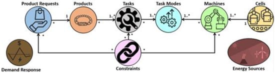
Figure 1.
Domain model of the proposed methodology.
- task—an activity that needs to be executed to create a product;
- task mode—a combination of energy and time profiles regarding the execution of a given task, where each task can have multiple task modes associated, which means that a single task can be executed in different ways;
- machine—a representation of a machine that has a list of compatible task modes that it can execute, thus being indirectly associated with tasks;
- cell—portrays a collection of machines where a product can be built;
- product—a representation of a product describing the necessary tasks to be completed before the product is considered finished;
- product request—the request of a new product to be produced along with the quantity needed;
- energy source—the energy source availability amount and price, an energy source can represent external providers (e.g., aggregator or retailer) or local generation (e.g., photovoltaic), the energy prices of local renewable sources can be set to zero;
- demand response—identifies the demand response program that the production line will participate in;
- constraint—a condition that will be respected by the algorithm.
The use of constraints is not mandatory, but it is needed to represent realistic cases where physical restrictions are in place. Currently, the proposed algorithm has the following constraints available to use:
- task order—defines a sequence between two tasks, for example, task B can only be executed after task A is completed;
- product task order—defines a sequence of tasks for a given product, allowing not only to have chains of repeated tasks but also have order constraints unique to a product. It is noteworthy that tasks that integrate this constraint do not need to comply with the task order constraint, due to logical fallacies;
- task collision—defines two tasks that cannot be executed at the same time;
- task setup—defines a setup action that needs to occur before task execution, this setup is defined by time and energy;
- time leap—can define breaks in time, the algorithm can schedule an entire week, but in cases where the production line does not operate 24 h a day, the time leap is used to indicate the last period before the break. This is necessary for tasks that cannot be stopped and must completely end before the break;
- interruptible task—defines tasks that can be paused and resumed any time;
- machine available frames—defines a maximum number of periods a machine is able to operate, for instance, it can be useful to prevent a machine from overloading;
- product request deadline—defines a deadline to which production of a given product request must be completed;
- product request task period range—defines a range of periods when a given task must be executed;
- product request cell choosing—defines the cell where the product request must be produced, bypassing the cell balancing optimization;
- energy limit—defines an energy limit, within a given interval, to be applied to energy sources with prices above zero. This constraint may also have monetary compensation for the full compliance with its limit;
- shift margin—the margin on energy price that the algorithm can use to allow the task to be close to each other, avoiding the existence of empty periods even if this increases the energy costs.
2.2. Production Line Optimization to Minimize Energy Cost
The production line energy cost optimization is divided into three main components: data processing characterized by the cell balancing; genetic algorithm represented by the initial population, crossover, mutation, and selection; and finally, the deterministic optimizations defined by the cost and shift optimizations. Figure 2 represents the flowchart of the production line energy cost optimization.
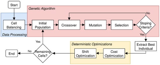
Figure 2.
Flowchart of the production line energy cost optimization.
2.2.1. Cell Balancing
The proposed algorithm starts by balancing the requests by the different cells available for manufacturing. This phase begins with the creation of a product request list, sorted by descending order of energy consumption needed to complete a product request. Because the tasks needed to complete a product request can be executed using different task modes with different energy profiles, an average is made considering all the possible task modes. An average of all the possible task modes is considered, above any other type of measure, since it better represents the overall processing time that a task can take.
Afterward, following the product request list, each request is assigned to the cell that has the lowest overall energy consumption, being the product request consumption added to the cell’s overall energy consumption. Moreover, the cell assignment process also takes into account if a cell is able to produce the requested product and if it has enough time frames to execute the product tasks.
Finally, after each request is assigned to a cell, each cell is executed by a genetic algorithm, followed by the deterministic-based optimizations. However, the cell optimizations are connected among them by the general data and to comply with general constraints, such as the availability of renewable energy sources that are shared among cells, and energy limit constraints that are applied to the plant floor (i.e., the sum of cells).
The cell balancing optimization focuses on maximizing energy distribution among cells, thus allowing more flexible request management, which in turn reduces the overall energy cost.
2.2.2. Initial Population
The genetic algorithm starts by initially creating an initial random population, respecting all the imposed constraints. To facilitate the creation of an individual and decrease the rate of not feasible individuals, the algorithm takes into account the compatible machines for each task and prioritizes tasks with a lower number of compatible machines and with a higher processing time. After knowing the list of tasks associated with each machine, a two-dimensional matrix is created, which represents the work plan of the job shop, where each line represents the plan of a machine, and each column represents a period. Figure 3 shows an example of such a matrix, where tasks are identified by colors and their identifiers.
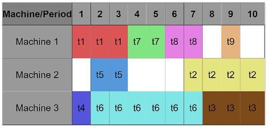
Figure 3.
Example of an individual matrix (machine/period), from the genetic algorithm, where tasks are identified by colors and their identifiers.
After an individual matrix is generated and at least one constraint is not respected, there are implemented methods that try to repair the generated individual (i.e., by shifting tasks left or right, swapping tasks). In case the repair is not successful, another individual is generated.
Since the number of columns (time period) corresponds to the time window of the schedule, every matrix from each cell will have the same number of columns but may differ in the number of rows, as cells can have a different number of machines associated.
2.2.3. Crossover
A new generation begins with the crossover of the population of the previous generation. The crossover performed is done between two individuals randomly chosen, which have not yet been crossed; this is guaranteed through a permutation of the population before the crossover is done. The crossover is a two-dimensional type, which will try to balance the tasks coming from each parent (individual). The crossover between two individuals (parents) begins with the formation of the list of tasks for the entire plan, ordered in decreasing order of processing time, and if they have equal times, it is ordered in ascending order of the number of machines compatible with the task. This, therefore, allows reducing the rate of invalid crosses between two individuals. In order of the task list, each task is taken and inserted in the child according to the parents’ coordinates; first, it starts with parent 1, then it changes to parent 2, then parent 1 again, and in general follows this sequence. Another child is made from the same parents but starts with parent 2 coordinates. Figure 4a represents the first four steps in a crossover, starting from parent 1.
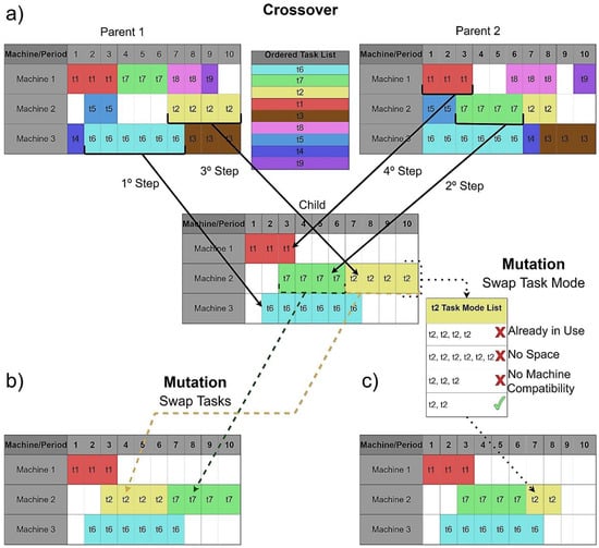
Figure 4.
Individuals’ crossover and mutation. (a) Example of the first 4 steps in a crossover, starting from parent 1; (b) example of a swapping tasks mutation; (c) example of a swapping the task mode on a task mutation.
After each crossover, where there are no incompatibilities between parent 1 coordinates and parent 2 coordinates, the resulted child is evaluated in terms of respecting all the imposed constraints. If at least one of the imposed constraints is not respected, the crossover is considered invalid.
In case of an invalid crossover, a perfect copy of either parent 1 or parent 2 is done to the child. This is done since afterward, in the selection phase, all the repeating individuals are eliminated, thus removing the child from the population pool. In short, if an invalid crossover occurs the child is never added to the population.
The most common approach to a crossover in a matrix is separating the parents based on a cutting point(s), in either a column or row manner, in other words, a probabilistic strategy. However, due to the problem at hand, many problems would arise such as task splitting, a high overlap of tasks, between the parents, and inconsistencies (i.e., tasks can have different processing times on each parent, due to task modes). Therefore, it was necessary to use a more deterministic approach to solve these issues.
2.2.4. Mutation
Using the population obtained from the crossover, a mutation is performed. In this procedure, the algorithm takes each individual, and according to the percentage of mutation defined in the input data, it decides whether or not the mutation will be applied to a given individual. However, if the mutation is applied, one of three different types, using equal probabilities, is randomly chosen:
- swapping tasks, changing two tasks in order of execution and/or machine. Figure 4b represents an example of a swapping tasks mutation;
- swapping the task mode on a task, affecting energy consumption and processing time. Figure 4c represents an example of a swapping the task mode on a task mutation;
- the combination of both swapping tasks and task mode.
If a mutation leads to an invalid individual (i.e., not respecting a certain constraint) then the mutation is reversed and another mutation, affecting different tasks in the schedule, is tried. Nevertheless, if no valid individual can be reached with a mutation, after a short number of tries, no mutation is done.
2.2.5. Selection
The selection phase begins with the union of the new and the old populations, that is, the crossed and mutated population with the initial population of the previous generation. Additionally, repetitions of individuals are eliminated. Then, each individual is evaluated using the following fitness equation:
where represents a time frame (period), the time window of the schedule, portrays a machine index, and the maximum number of machines available. Both and can be translated into the cartesian coordinates, and , respectively, to navigate in the schedule matrix. The energy consumption of a task in a given period is represented by , defines the locally generated energy, which is energy free of charge (e.g., photovoltaic generation), and represent the energy prices. The energy cost of each individual, represented in the denominator of the fraction, is determined as a result of the energy balance () multiplied by the respective energy price.
The selection of the best individuals is made according to the input parameter of the algorithm, chosen by the user. The remaining individuals (i.e., population size less ) are obtained from non-elite tournaments. Each tournament consists of two individuals randomly chosen, where they compete based on their fitness scores. The algorithm calculates the chance of individual 1 winning the tournament using the equation
where and represent the fitness of the individual 1 and individual 2, respectively.
Then, a random decimal number between 0 and 1 is generated. If the generated decimal is lower than the chance of individual 1 winning, Equation (2), then individual 1 is declared the winner. Otherwise, individual 2 leaves victorious. Therefore, the individual with the highest fitness, which in turn has the lowest cost, is the one most likely to be chosen.
2.2.6. Extract Best Individual
At the end of the selection phase, the next generation begins with the population obtained from this selection, and all the procedures mentioned above are repeated. Finally, after a stop condition is met, the best individual is extracted from the last population of the genetic, that is, the lowest cost job shop schedule, generated by the genetic algorithm. Thus, in general, the genetic algorithm, through Equation (1), which represents the objective function, tries to minimize the energy cost of the elaborated job shop schedule as much as possible, taking into consideration restrictions, such as task orders, task collisions, energy limits, request deadlines, PV generation, etc.
2.2.7. Cost Optimization
After the execution of the genetic algorithm, a post-processing phase is required to adjust/further optimize the result given by the genetic algorithm through a deterministic approach.
The cost optimization function will analyze the result of the genetic algorithm, and it will identify periods with lower energy costs that do not have an assigned task, then it will try to place the tasks with higher energy consumption to the lower energy cost time slots. If tasks can be exchanged while resulting in a cost reduction and respecting all the constraints, the exchange is carried out. This optimization function uses the energy cost resulted from the prices of all energy sources available, including local renewable energy sources.
2.2.8. Shift Optimization
Shift optimization is made by sliding tasks in time to reduce the time between them. This optimization differences from the cost optimization because no task will be changed, only slide to near periods. Its main purpose is to join tasks, reducing the time between them. For each isolated task (i.e., with empty periods on the left or on the right), the shift optimization will try to shift it to the left, and if all constraints are valid and energy costs decrease, or are maintained within the shift margin constraint level, the shift is performed. If the left shifting is not possible, then the shift optimization tries to shift the task to the right, applying the same conditions described before. Figure 5 shows an example of the shift optimization performed to a machine work plan.
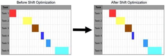
Figure 5.
Example of the shift optimization for a machine work plan.
2.3. Demand Response Participation Using Production Line Flexibility
The proposed algorithm enables the use of flexibility in production lines for demand response participation. To use the flexibility of the production line, three main parts are needed: data processing, genetic algorithm, and determinist optimizations. This process is similar to the one presented in Figure 2, with the addition of the block of flexible data processing introduced to enable the use of flexibility in the scheduling optimization. Figure 6 shows how flexibility is used in the proposed methodology.
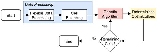
Figure 6.
Flowchart for flexibility usage.
The flowchart of Figure 6 is only applied to schedule plans that were already resulted from the proposed algorithm of Section 2.2. For plans that did not already start, the demand response event can be integrated directly into the optimization using the energy limit constraint. For plans that had already started being executed, then we need to apply the flowchart of Figure 6.
In the flexible data processing module, the already-made schedule is divided into two segments: one that represents the schedule with the tasks that were already started or executed, and a second segment with the schedule of tasks that are planned but not yet started. The second segment is then parsed to create an input for the genetic algorithm, taking into account the task already executed in the first schedule segment and updating all the constraints. However, before the genetic algorithm execution, the proposed solution applies the cell balancing method described in Section 2.2.1.
The genetic algorithm is executed with an additional constraint: energy limit. This constraint defines a limit within a given interval of time frames of energy we can get from the energy provider that had launched the demand response event. Considering this constraint, the genetic algorithm is able to produce a result compliant with the demand response event.
The same cost and shift optimizations, described in Section 2.2.7 and Section 2.2.8, are applied in the result of the genetic algorithm. Finally, the new schedule is attached to the schedule of the first segment, with the tasks already started or executed, and the final schedule is presented to the user.
3. Results and Discussion
The case study of this paper uses real production data, provided by a textile company that manufactures hang tags. Their working schedule is from 7:00 to 23:00 each working day, from Monday to Saturday. The case study uses a period of 5 min for all task durations and energy data, thus an overall time window of 1152. The case study considers six working days, Monday to Saturday, from 7:00 to 23:00 each day. The scheduling algorithm was used for three machines that share the same cell, thus each individual matrix, in the genetic algorithm, is 3 rows by 1152 columns. Table 1 describes the machines according to the tasks they are able to execute.

Table 1.
Tasks that each machine executes.
The case study used four constraints: time leap, task order, task collision, and product request deadline. The time leap constraint was applied in every period that represents a day transition, time periods 192, 384, 576, 768, and 960, which corresponds to the final time period in each day (23:00 of Monday, Tuesday, Wednesday, Thursday, and Friday). A task order constraint where every task “Harden [1.5]” must be preceded by a task “Harden [2]”, a task collision constraint between tasks “Sublimation” and “Harden [2]”, and a product request deadline, in a product, of time period 960, which corresponds to a deadline of 23:00 of Friday. During the week, 132 units of 14 products were requests. The genetic algorithm was executed using a population size of 20, an elite size of 3, a mutation rate of 5%, and with a stop condition of 2 h, which for this case study averages around 1500 generations. Regarding the full access of the datasets used in this paper, the full description of the input data and results of the genetic algorithm can be seen in [30], while the results of the demand response program can be seen in [31].
3.1. Energy Cost Optimization
The scheduling of the production line considers the scenario described above and two energy sources, including local renewable generation provided by photovoltaic panels. Market prices considered are MIBEL (Iberian Electricy Market) prices from the 7 January 2019 to the 12 January 2019, and the sale value corresponds to 50% of the buying. The local renewable generation profile was obtained from the 6 June 2020 to the 11 June 2020 in a 3 kW peak photovoltaic installation in Portugal. The algorithm was executed in 2 h on a computer with an Intel® Core™ i3-7020U processor running at 2.30 GHz using 8 GB of RAM, running Windows 10 Home version 2004. Its main results can be seen in Figure 7 where tasks are distributed by the available machines and along the time periods available. Due to size limitations, it was not possible to discriminate all the tasks names; nonetheless, the complete open data were published in [30]. Machine occupation rates of 59.72%, 81.77%, and 79.86% were reached for machines 118, 119, and 120, respectively.
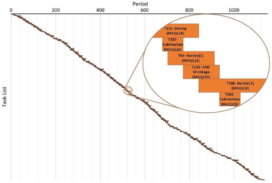
Figure 7.
Gantt diagram of the scheduled plan.
Figure 8 shows the consumption aggregation of production profiles considering the result of the scheduling optimization. Energy consumed is obtained through the algorithm, which provides stats. The market prices reflect the MIBEL prices from the 7 January 2019 to the 12 January 2019. The solar generation profile was obtained from the 6 June 2020 to the 11 June 2020 in a 3 kW peak photovoltaic installation in Portugal. It is noteworthy that the higher the energy price in a given period the lower the energy consumed, indicating that the algorithm was able to shift the tasks to lower energy price periods. The local energy generation, provided by photovoltaic panels, was used as much as possible by the algorithm, reducing the demand for external supplies with higher energy prices.
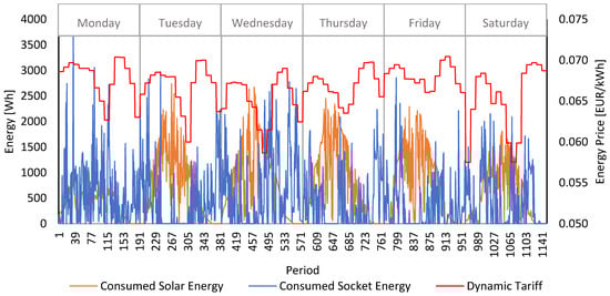
Figure 8.
Energy consumption with energy costs.
The overall performance of the algorithm can be seen in Figure 9 where the best individual of each generation is presented according to its overall cost. The results followed a decreasing logarithmic function, showing a good performance.
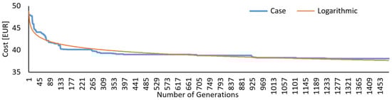
Figure 9.
Cost per generation of the genetic algorithm.
3.2. Demand Response Application
Using the previous data as the starting point, an announcement of a demand response program was simulated on Friday at 6:00, describing a demand response event from Friday at 21:00 (period 937) to Friday at 23:00 (period 960), where each period represents five minutes. The demand response program imposed a limit consumption, during its event, of 2.5 kWh. The announcement of the demand response allowed the use of the proposed solution to limit energy consumption. For that, the algorithm described in Section 2.3 was executed at period 769 (Friday at 7:00). Figure 10 shows the machines’ energy consumption before and after the demand response participation rescheduling of tasks. The full dataset can be seen in [31]. The demand response event is represented with an orange rectangle, while the rescheduling consumption is represented by an orange line.
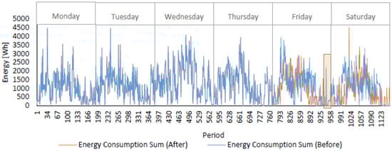
Figure 10.
Energy consumption of the demand response event.
Figure 11 shows the machines’ energy consumption difference, considering as base the previously scheduled plan, and it is compared to the new scheduled plan. It is possible to see that during the demand response event (orange rectangle) the consumption decreased to not go above 2.5 kWh.
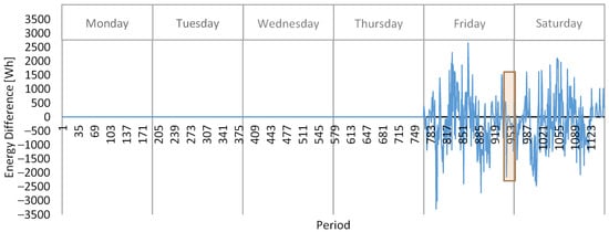
Figure 11.
Energy consumption difference (after − before) of the demand response event.
The tasks were rescheduled away from the demand response event period. Figure 12 shows a magnification of before and after the demand response, where the full before scenario is shown in Figure 7. As can be seen, the algorithm started the demand response event with scheduled tasks, but when it reached a total energy of near 2.5 kWh, no more tasks were executed.
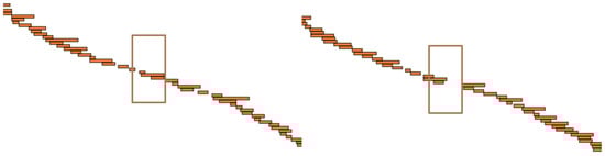
Figure 12.
Before and after Gantt diagrams of the demand response event, respectively, from period 848 to period 1058.
4. Conclusions
Industries nowadays operate in a challenging dynamic environment where time commitments are very rigid. Moreover, all the costs should be considered and minimized. This includes the energy costs and the opportunities coming from the participation in demand response events. Moreover, the electricity prices changing in real-time should be followed.
Accordingly, the present paper proposed and implemented an approach based on a genetic algorithm to minimize operation costs of a production line, respecting a set of constraints related to the product delivery and to the energy aspects. The implemented approach was able to handle this complex optimization problem in a time frame fast enough to receive demand response and energy prices in real-time and update the production planning taking into account such inputs.
The obtained results highlight the robustness of the implemented methodology to handle a set of three machines operating sequentially to deliver products in a one-week time frame. Given the flexibility of time available to perform each task, it was possible to allocate each task considering its specific consumption looking at the prices in real-time and the demand response event. In this way, the production cost was minimized.
Author Contributions
Conceptualization, C.R. and Z.V.; methodology, L.G., P.F., C.R. and Z.V.; software, B.M.; validation, B.M., L.G., P.F., C.R., R.C. and Z.V.; formal analysis, B.M., L.G. and P.F.; investigation, B.M., L.G. and P.F.; resources, C.R. and Z.V.; data curation, B.M. and R.C.; writing—original draft preparation, B.M., L.G. and P.F.; writing—review and editing, C.R., R.C. and Z.V.; visualization, B.M. and L.G.; supervision, C.R. and Z.V.; project administration, C.R., R.C. and Z.V.; funding acquisition, C.R., R.C. and Z.V. All authors have read and agreed to the published version of the manuscript.
Funding
This work has received funding from Portugal 2020 under SPEAR project (NORTE-01-0247-FEDER-040224) and from FEDER Funds through COMPETE program and from National Funds through (FCT) under the project UIDB/00760/2020, and CEECIND/02887/2017.
Institutional Review Board Statement
Not applicable.
Informed Consent Statement
Not applicable.
Data Availability Statement
The data presented in this study are available in [30,31].
Conflicts of Interest
The authors declare no conflict of interest.
References
- Guerrero, J.; Gebbran, D.; Mhanna, S.; Chapman, A.C.; Verbič, G. Towards a transactive energy system for integration of distributed energy resources: Home energy management, distributed optimal power flow, and peer-to-peer energy trading. Renew. Sustain. Energy Rev. 2020, 132, 110000. [Google Scholar] [CrossRef]
- Schweiger, G.; Eckerstorfer, L.V.; Hafner, I.; Fleischhacker, A.; Radl, J.; Glock, B.; Wastian, M.; Rößler, M.; Lettner, G.; Popper, N.; et al. Active consumer participation in smart energy systems. Energy Build. 2020, 227, 110359. [Google Scholar] [CrossRef]
- Zhang, Y.; Campana, P.E.; Yang, Y.; Stridh, B.; Lundblad, A.; Yan, J. Energy flexibility from the consumer: Integrating local electricity and heat supplies in a building. Appl. Energy 2018, 223, 430–442. [Google Scholar] [CrossRef]
- Afzalan, M.; Jazizadeh, F. Residential loads flexibility potential for demand response using energy consumption patterns and user segments. Appl. Energy 2019, 254, 113693. [Google Scholar] [CrossRef]
- Gomes, L.; Spínola, J.; Vale, Z.; Corchado, J.M. Agent-based architecture for demand side management using real-time resources’ priorities and a deterministic optimization algorithm. J. Clean. Prod. 2019, 241, 118154. [Google Scholar] [CrossRef]
- Gherghea, I.C.; Bungau, C.; Negrau, C.C. Best Practices to Increase Manufacturing Productivity—Comparative study. In Proceedings of the 9th International Conference on Manufacturing Science and Education (MSE 2019), Sibiu, Romania, 5–7 June 2019. [Google Scholar] [CrossRef]
- Ramos, C.; Barreto, R.; Mota, B.; Gomes, L.; Faria, P.; Vale, Z. Scheduling of a textile production line integrating PV generation using a genetic algorithm. Energy Rep. 2020, 6, 148–154. [Google Scholar] [CrossRef]
- Wang, B.; Tao, F.; Fang, X.; Liu, C.; Liu, Y.; Freiheit, T. Smart Manufacturing and Intelligent Manufacturing: A Comparative Review. Engineering 2020. [Google Scholar] [CrossRef]
- Nguyen, S.; Mei, Y.; Zhang, M. Genetic programming for production scheduling: A survey with a unified framework. Complex Intell. Syst. 2017, 3, 41–66. [Google Scholar] [CrossRef]
- Ángel Vega-Velázquez, M.; García-Nájera, A.; Cervantes, H. A survey on the Software Project Scheduling Problem. Int. J. Prod. Econ. 2018, 202, 145–161. [Google Scholar] [CrossRef]
- Branke, J.; Nguyen, S.; Pickardt, C.W.; Zhang, M. Automated Design of Production Scheduling Heuristics: A Review. IEEE Trans. Evol. Comput. 2016, 20, 110–124. [Google Scholar] [CrossRef]
- Khorram, M.; Faria, P.; Vale, Z.; Ramos, C. Sequential Tasks Shifting for Participation in Demand Response Programs. Energies 2020, 13, 4879. [Google Scholar] [CrossRef]
- Luo, Z.; Hong, S.-H.; Kim, J.-B. A Price-Based Demand Response Scheme for Discrete Manufacturing in Smart Grids. Energies 2016, 9, 650. [Google Scholar] [CrossRef]
- Abedinnia, H.; Glock, C.H.; Schneider, M.D. Machine scheduling in production: A content analysis. Appl. Math. Model. 2017, 50, 279–299. [Google Scholar] [CrossRef]
- Fuchigami, H.Y.; Rangel, S. A survey of case studies in production scheduling: Analysis and perspectives. J. Comput. Sci. 2018, 25, 425–436. [Google Scholar] [CrossRef]
- Đurasević, M.; Jakobović, D.; Knežević, K. Adaptive scheduling on unrelated machines with genetic programming. Appl. Soft Comput. 2016, 48, 419–430. [Google Scholar] [CrossRef]
- Wu, X.; Consoli, P.; Minku, L.; Ochoa, G.; Yao, X. An Evolutionary Hyper-heuristic for the Software Project Scheduling Problem. In Parallel Problem Solving from Nature—PPSN XIV. PPSN 2016; Lecture Notes in Computer Science; Handl, J., Hart, E., Lewis, P., López-Ibáñez, M., Ochoa, G., Paechter, B., Eds.; Springer: Cham, Switzerland, 2016; Volume 9921. [Google Scholar] [CrossRef]
- Shen, X.N.; Minku, L.L.; Marturi, N.; Guo, Y.N.; Han, Y. A Q-learning-based memetic algorithm for multi-objective dynamic software project scheduling. Inf. Sci. 2018, 428, 1–29. [Google Scholar] [CrossRef]
- Xiao, J.; Gao, M.-L.; Huang, M.M. Empirical Study of Multi-objective Ant Colony Optimization to Software Project Scheduling Problems. In Proceedings of the 2015 Annual Conference on Genetic and Evolutionary Computation (GECCO ’15), New York, NY, USA, 11–15 July 2015. [Google Scholar] [CrossRef]
- Chen, J.; Huang, G.Q.; Wang, J.Q. Synchronized scheduling of production and outbound shipping using bilevel-based simulated annealing algorithm. Comput. Ind. Eng. 2019, 137, 106050. [Google Scholar] [CrossRef]
- Ruiz Duarte, J.L.; Fan, N.; Jin, T. Multi-process production scheduling with variable renewable integration and demand response. Eur. J. Oper. Res. 2020, 281, 186–200. [Google Scholar] [CrossRef]
- Chen, B.; Zhang, X. Scheduling with time-of-use costs. Eur. J. Oper. Res. 2019, 274, 900–908. [Google Scholar] [CrossRef]
- Santana-Viera, V.; Jimenez, J.; Jin, T.; Espiritu, J. Implementing factory demand response via onsite renewable energy: A design-of-experiment approach. Int. J. Prod. Res. 2015, 53, 7034–7048. [Google Scholar] [CrossRef]
- Li, B.; Tian, Y.; Chen, F.; Jin, T. Toward net-zero carbon manufacturing operations: An onsite renewables solution. J. Oper. Res. Soc. 2017, 68, 308–321. [Google Scholar] [CrossRef]
- Gomes, L.; Faria, P.; Morais, H.; Vale, Z.; Ramos, C. Distributed, Agent-Based Intelligent System for Demand Response Program Simulation in Smart Grids. IEEE Intell. Syst. 2014, 29, 56–65. [Google Scholar] [CrossRef]
- Faria, P.; Vale, Z. Demand response in electrical energy supply: An optimal real time pricing approach. Energy 2011, 36, 5374–5384. [Google Scholar] [CrossRef]
- Vale, Z.; Morais, H.; Faria, P.; Ramos, C. Distribution system operation supported by contextual energy resource management based on intelligent SCADA. Renew. Energy 2013, 52, 143–153. [Google Scholar] [CrossRef]
- Bharathi, C.; Rekha, D.; Vijayakumar, V. Genetic Algorithm Based Demand Side Management for Smart Grid. Wirel. Pers. Commun. 2017, 93, 481–502. [Google Scholar] [CrossRef]
- Fernandes, F.; Sousa, T.; Silva, M.; Morais, H.; Vale, Z.; Faria, P. Genetic algorithm methodology applied to intelligent house control. In Proceedings of the 2011 IEEE Symposium on Computational Intelligence Applications In Smart Grid (CIASG), Paris, France, 11–15 April 2011. [Google Scholar] [CrossRef]
- Mota, B.; Gomes, L.; Faria, P.; Ramos, C.; Vale, Z. Production line dataset for task scheduling and energy optimization—Schedule Optimization (Version 0.1). Zenodo 2020. [Google Scholar] [CrossRef]
- Mota, B.; Gomes, L.; Faria, P.; Ramos, C.; Vale, Z. Production line dataset for task scheduling and energy optimization—Demand Response Participation (Version 0.1). Zenodo 2020. [Google Scholar] [CrossRef]


Publisher’s Note: MDPI stays neutral with regard to jurisdictional claims in published maps and institutional affiliations. |
© 2021 by the authors. Licensee MDPI, Basel, Switzerland. This article is an open access article distributed under the terms and conditions of the Creative Commons Attribution (CC BY) license (http://creativecommons.org/licenses/by/4.0/).