Influence of Non-Linearity in Losses Estimation of Magnetic Components for DC-DC Converters

Abstract

In this paper, the problem of estimating the core losses for inductive components is addressed. A novel methodology is applied to estimate the core losses of an inductor in a DC-DC converter in the time-domain. The methodology addresses both the non-linearity and dynamic behavior of the core magnetic material and the non-uniformity of the field distribution for the device geometry. The methodology is natively implemented using the LTSpice simulation environment and can be used to include an accurate behavioral model of the magnetic devices in a more complex lumped circuit. The methodology is compared against classic estimation techniques such as Steinmetz Equation and the improved Generalized Steinmetz Equation. The validation is performed on a practical DC-DC Buck converter, which was utilized to experimentally verify the results derived by a model suitable to estimate the inductor losses. Both simulation and experimental test confirm the accuracy of the proposed methodology. Thus, the proposed technique can be flexibly used both for direct core loss estimation and the realization of a subsystem able to simulate the realistic behavior of an inductor within a more complex lumped circuit.

1. Introduction

DC-DC power converters are widely used in many electrical and electronic applications. The diffusion of wide-bandgap semiconductors, characterized by fast switching transients is increasing the operating frequency of DC-DC converters allowing for higher power densities [1,2,3].

Magnetic components are the bulkiest components of power converters, and their design must be accurate to avoid excessive weights and volumes [4]. Much effort has been spent in investigating the inductor losses generated in its winding and on its core [5]. The latter can result in both non-linear and dynamic behavior, because of the saturation and magnetic hysteresis phenomena [6]. This behavior is, in general, due to the material [7]. Considering the device geometry (i.e., the magnetic core shape), additional complexity arises due to the non-uniform distribution of the magnetic induction field across the core section, and this issue has only been partially investigated [8]. Considering these factors during the design of power converters is very difficult. For this reason, some manufacturers aim at constructive solutions that make the behavior of the magnetic component as simple as possible. In addition, they are looking for solutions with uniform distribution of magnetic field [9].

By neglecting the non-uniform magnetic induction distribution and only referring to the component data sheets, the designers are guided to choose a non-optimal magnetic component, which, under practical operating conditions, results in a worse performance than expected. Moreover, it results in oversized and overweight designs [10,11,12,13].

An optimal sizing can be achieved through calculation tools able to consider non-linearity, magnetic hysteresis, and the real non-uniform distribution of the magnetic induction in the component core, with acceptable accuracy [14,15,16].

The modeling of non-linearity and hysteresis in magnetic materials is achieved with different deterministic approaches, both at the micromagnetic and macromagnetic levels, but also with stochastic approaches based on specific applications of artificial intelligence [17]. The determination of distribution of magnetic field inside an inductor core is also possible by using numerical tools based on finite element methods [18,19].

Many difficulties need to be overcome when both the non-linearity, the magnetic hysteresis, and the distribution of the magnetic induction in the core must be considered in a time-domain simulation [20].

The dominant problem is that the magnetic component analysis must be set in the time-domain, and due to the non-linear nature of the equations regulating its behavior, the numerical solution (i.e., the response of the material/device) must be obtained with iterative methods. If the core geometry is considered, the discretization through the meshes of the magnetic core must be sufficiently dense [21]. Assuming this magnetic component is part of a larger time-domain simulation (e.g., a power converter), this computational process is repeated for every time-step of the simulation, resulting in a very computationally demanding scenario [22]. The computational burden of the simulation is often further increased by the very short time steps chosen to avoid numerical instability.

An interesting approach to estimate the dynamic power losses is given in [23], where the losses are calculated by a specifically designed Spice circuit, which considers the dynamic power losses. This approach is based on a model which is useful for the simulation of the behavior of DC-DC converters and allows the magnetic non-linearity to be considered along with the hysteresis and the non-uniformity of the magnetic induction. In [23], the operation of the core close to the saturation point is not considered, and this yields inaccuracies in the determination of the inductor current waveforms, which are strongly distorted in DC-DC converters. This problem has been faced in an improved model where the capability of reproducing magnetic hysteresis cycles has been introduced by referring to the non-linear behavior of the material when operated near the magnetic saturation point [24].

This paper aims to apply the approach utilized in [24], for the investigation of a DC-DC Buck converter. The proposed work focuses on the proposed model consistency when embedded in a larger design simulation. To validate this methodology, an experimental Buck converter circuit was built, and current measurements were acquired in the choke inductor. Core losses were estimated through three different techniques: the first one is based on the classic Steinmetz Equation (SE), which considers the frequency behavior of the material, yet lacks the capability of time-domain simulation under arbitrarily distorted waveforms. The second is the improved Generalized Steinmetz Equation (iGSE) technique, which introduces a methodology to apply the SE to a time-domain simulation under distorted waveform but lacks the geometric account for non-uniform field distribution in the device. The last one is the Time-Domain Core Loss with Non-Uniform Field (TDNU) technique based in the model as given in [24,25]. This technique seems also to be promising to be included in high component number circuit designs and can benefit from the optimized integration engines coupled with circuit simulation software. The paper is structured as follows. First, the two state-of-the-art methodologies used for the comparison are discussed. Then, the proposed methodology is presented, underlying the improvements introduced with respect to the classic literature approaches. In the following section, the DC-DC Buck converter design and the experimental workbench implementation are described, with particular attention to the inductor characteristics and the algorithmic approach used to estimate the losses using the three techniques. Measurements and estimated losses are then presented, along with the reconstructed hysteresis profiles, for a DC-DC Buck converter operated under different operating conditions. Conclusion and final remarks close the manuscript.

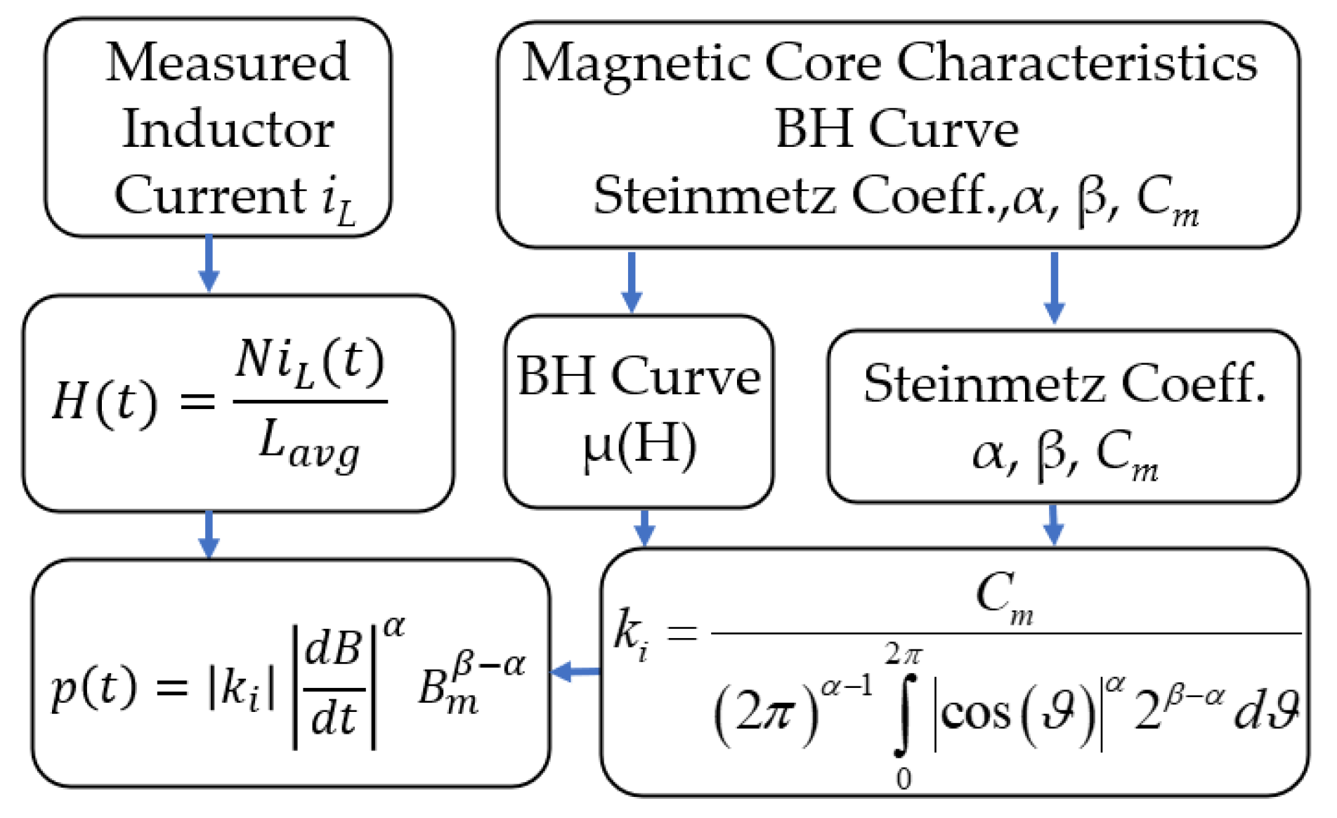
2. Steinmetz Equations and Improved Generalized Steinmetz Approach

Core loss estimation can be achieved through the direct application of the Steinmetz equation. This equation relates the losses to the frequency of the excitation and the intensity of the magnetic induction, and thanks to its simplicity, represents a good method to predict the core losses under sinusoidal excitation. The average power loss is given by

$$P=C_m{f}^{\alpha }{B}_m^{\beta }$$

(1)

where C_m, α and β are the Steinmetz coefficients, f is the frequency of the excitation and B_m is the RMS value of the core magnetic flux density [26,27,28]. The main limit of this formula is that it results in an accurate estimation only under sinusoidal induction [26,27]. This limitation makes this formula difficult to use in time-domain simulations of non-linear devices operated at distorted currents (and, thus, H-B fields). To solve this limitation, several models were proposed. One of the most promising one is that based on the improved Generalized Steinmetz Equation (iGSE) [29,30].

Here, the average core loss is computed as

$$P=\frac{1}{T}{\displaystyle \underset{0}{\overset{T}{\int }}}\left|k_i\right|{\left|\frac{dB}{dt}\right|}^{\alpha }{\left|B_m\right|}^{\beta -\alpha }dt$$

(2)

where B_m is the peak-to-peak flux density and

$$k_i=\frac{C_m}{{\left(2\pi \right)}^{\alpha -1}{\displaystyle \underset{0}{\overset{2\pi }{\int }}{\left|\cos \left(\vartheta \right)\right|}^{\alpha }}{2}^{\beta -\alpha }d\vartheta }$$

(3)

This methodology accounts for an arbitrarily time-varying magnetic field, and for this reason, it is suitable for inclusion in time-domain simulation of magnetic materials. However, iGSE assumes a uniform distribution of the magnetic induction inside the core. It can be noted that the iGSE technique, differently from the SE approach, allows for a time-domain estimation of the core losses and can be therefore implemented in Spice environment.

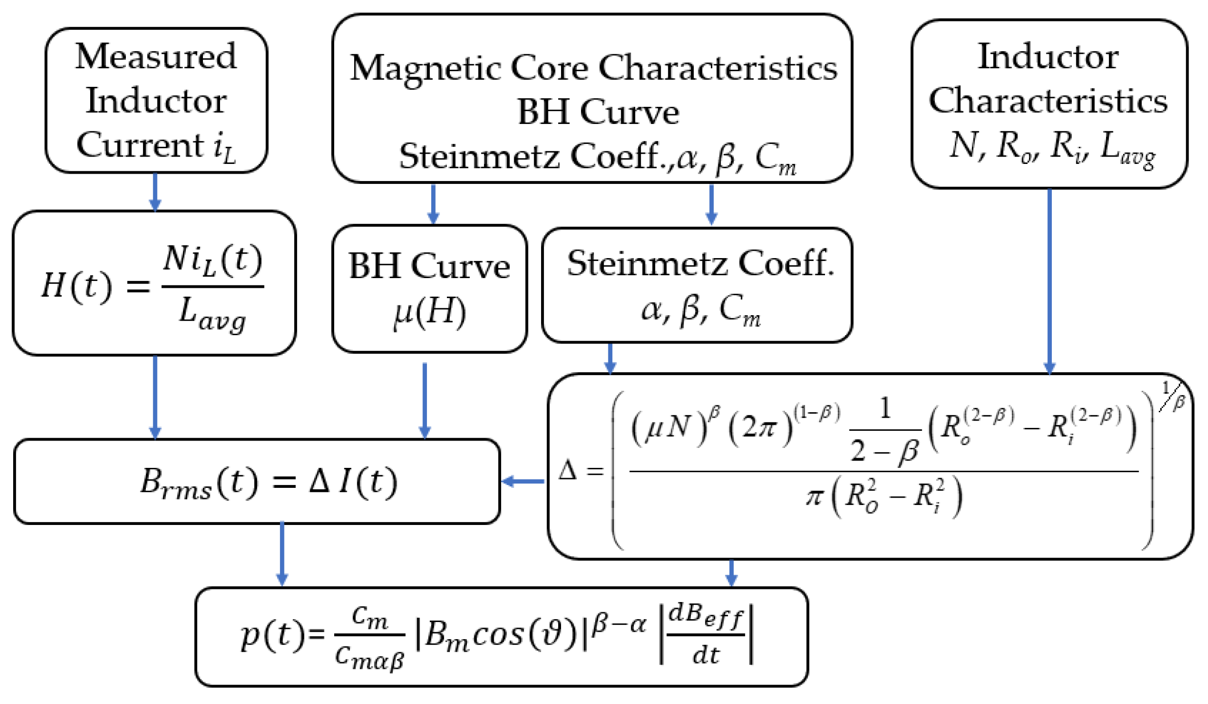
3. Time-Domain Core Loss with Non-Uniform Field (TDNU)

A more recent method utilized to obtain a Time-Domain Core Loss estimation under non-sinusoidal excitation was presented in [23,24]. This approach allows to estimate the core power losses by using a time-domain approach rather than one based on a frequency-domain analysis. As a result, non-linearities can be considered, and estimations can be performed even with non-sinusoidal waveforms. In addition, by estimating the instantaneous power loss p(t), it is possible to predict the core losses during both the transient and steady-state operation. In addition, this approach takes into account the non-uniform magnetic field distribution inside the magnetic core. The instantaneous core loss is derived as

$$p(t)=\frac{C_m}{C_{\alpha \beta }}{\left|B_m\cos \vartheta \right|}^{\left(\beta -\alpha \right)}\left|\frac{d{B}_{eff}}{dt}\right|,$$

(4)

where

$$C_{\alpha \beta }={\left(2\pi \right)}^{\alpha }\frac{2}{\pi }{\displaystyle \underset{0}{\overset{\pi /2}{\int }}{\left(\cos \vartheta \right)}^{\alpha }d\vartheta },$$

(5)

and B_eff represents an equivalent flux density which considers the shape and the geometry of the core and approximates the effects of the non-uniformity of the magnetic field inside the core. This method consists of matching the area formed by an equivalent elliptical loop with the original hysteresis loop starting from the standard core loss coefficients. In (5), the parameter cos ϑ is computed as

$$\cos \vartheta (t)=\sqrt{1-\left(\frac{B_{eff}(t)-B_{DC}}{B_m}\right)}$$

(6)

where B_DC represents the DC induction bias. To compute the effective magnetic flux density B_eff, a parameter Δ, called “field factor”, is defined. This parameter depends on the magnetic core geometry and material, and relates the effective flux density with the current through the inductor according to

$$B_{eff}(t)=\Delta \cdot I\left(t\right).$$

(7)

For a toroidal core, the field factor can be calculated as in [24]

$$\Delta ={\left(\frac{{\left(\mu N\right)}^{\beta }{\left(2\pi \right)}^{\left(1-\beta \right)}\frac{1}{2-\beta }\left(R_o^{\left(2-\beta \right)}-R_i^{\left(2-\beta \right)}\right)}{\pi \left(R_O^2-R_i^2\right)}\right)}^{\raisebox{1ex}{$1$}\!\left/ \!\raisebox{-1ex}{$\beta $}\right.}$$

(8)

where µ= µ₀ µ_r is the magnetic material permeability, N is the number of turns, and R_o and R_i are the outer and inner radius of the toroidal core.

Note that if β = 1, the field factor simplifies as

$$\Delta =\frac{\mu N}{\pi \left(R_O^2-R_i^2\right)}$$

(9)

Under this condition, (7) becomes

$$B_{eff}(t)=\frac{\mu N}{\pi \left(R_O^2-R_i^2\right)}\cdot I\left(t\right).$$

(10)

which fully describes the case with a uniform magnetic field distribution. To properly compute the power loss p(t) given by (4), the actual values of B_m and B_DC must be cyclically updated. Since the proposed method works in the time-domain, the wipe out rule method is used: when the derivate of the magnetic flux density dB_eff/dt is zero, a maximum B_max or a minimum B_min value of the actual hysteresis loop is reached and, therefore, the values of B_DC and B_m are updated for a correct estimation of the power loss.

This technique has an important improvement which is of fundamental importance to perform time-domain simulations: in iGSE technique the estimation of the core loss is based on the knowledge of the mean average value of the magnetic flux B(t), while the method described in this section uses the effective magnetic flux B_eff which is estimated by using (7). Moreover, this approach can be used in a lumped elements circuit and, also, it allows the SPICE subsystem modeling the inductor to be integrated in a more complex circuit, as shown in Figure 1. A detailed description of the LTSpice circuit used to compute the time-domain core power loss can be found in [24].

In the next sections, starting from the measurements of a DC-DC Buck converter prototype, a comparison between the power core losses on the inductor using the Steinmetz Equation, the iGSE and the proposed approach is presented.

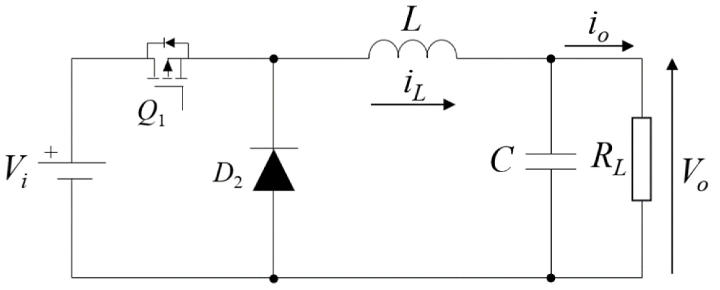
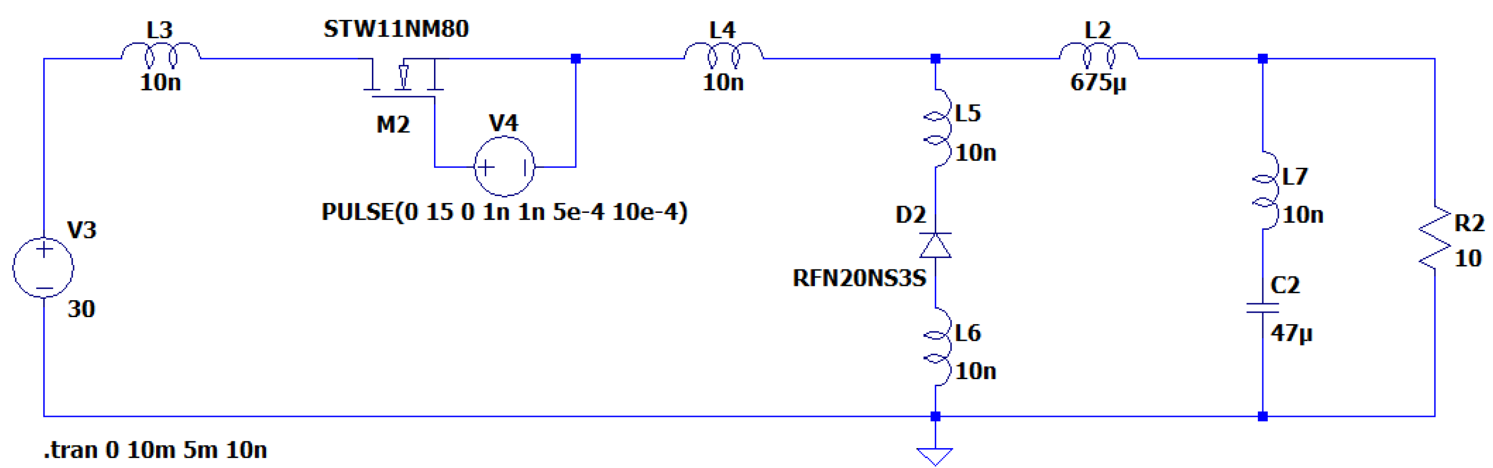
4. The Case Study: A DC-DC Buck Converter

To practically evaluate the accuracy of the three different techniques, the core loss on the inductor of a DC-DC Buck converter was analyzed. The electrical circuit of the buck converter is shown in Figure 2.

The KIT-CRD-3DD065P, Buck-Boost Evaluation Kit [31] was used to realize the experimental converter. The components are summarized in

Table 1. Buck Converter components.

Component	Description	Value
Power MOSFETs Q1	C3M0060065K	VDSmax = 650 V RDS(on) = 60 mΩ
Body Diode D2	C3M0060065K	VF = 4.8 V
Output Capacitor C	MAL205956479E3	47 µF
Load Resistance RL	HS100 1R J	10 Ω

.

Different operating frequencies and duty cycles were used to understand the performance of each core loss estimation technique and perform a comparison of their results. Indeed, the proposed topology works with unidirectional behavior. This turns out in a simpler driving system but excludes the possibility to evaluate the magnetic losses of typical bidirectional topologies. However, from the point of view of the core losses, the resulting waveforms will still include both the CCM and DCM condition, resulting in a complete behavioral analysis of the phenomenon.

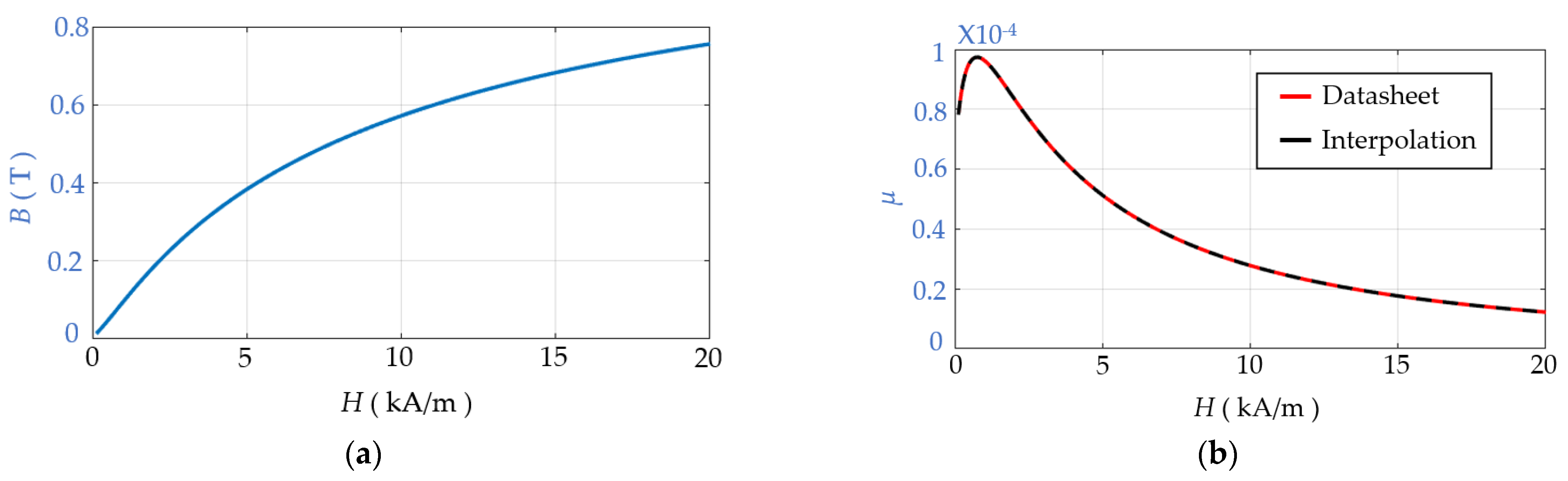
4.1. Inductor Characteristics

The inductor of Cree’s KIT-CRD-3DD065P Buck-Boost Evaluation Kit [31] is based on a toroidal high temperature rated powdered core, which results in a CWS-1SN-12877 inductor; the core material is KoolMu [32]. The geometric characteristics of the core are summarized in

Table 2. Inductor characteristics.

Component	Description
Number of Turns N	63
Inner Core Radius Ri	10.5 mm
Outer Core Radius Ro	20.5 mm
Height H	10 mm

along with the winding number of turns.

The anhysteretic curve of the magnetic core and the magnetic permeability are shown in Figure 3a,b, respectively.

The core Steinmetz coefficient are summarized in

Table 3. Steinmetz parameters from manufacturer.

Parameter	Value
Cm	44.30
β	1.988
α	1.541

.

By using in (5) the parameter values shown in Table 2, a coefficient C_αβ = 8.51 is obtained. The curve giving the magnetic core permeability µ shown in Figure 3 can be interpolated and expressed as a function of the magnetic field as follows

$$\mu =\frac{N(H)}{D(H)}=\frac{n_1{H}^3+n_2{H}^2+n_{3}H+n_4}{d_1{H}^3+d_2{H}^2+d_{3}H+d_4}$$

(11)

where, n₁ = 1.7650 × 10⁻¹⁷, n₂ = −1.8125 × 10⁻¹², n₃ = 2.551 × 10⁻⁷, n₄ = 6.379 × 10⁻⁵, d₁ = 1.4782 × 10⁻¹¹, d₂ = 5.520 × 10⁻⁷, d₃ = 0.0017, and d₄ = 1. As shown in Figure 3b, where the black dotted trace represents the plot of (11) and the red trace shows the real magnetic permeability the interpolation given by (7) perfectly matches the data sheet plot of the permeability.

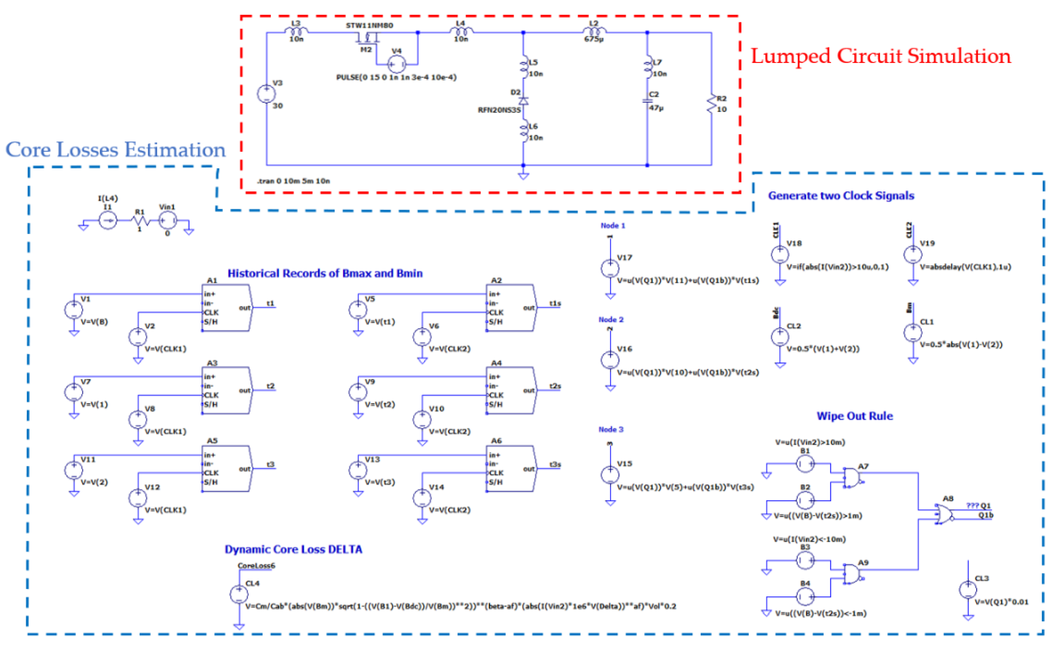
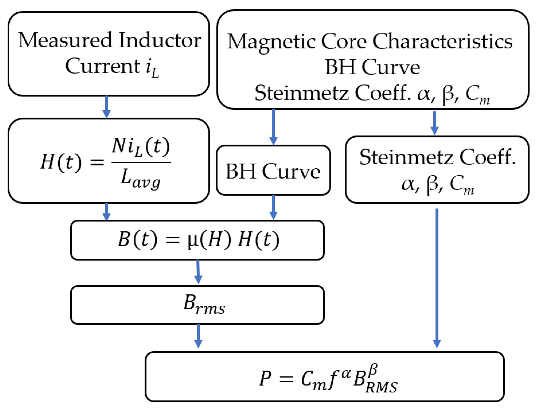
4.2. Core Loss Estimation Algorithms

The Steinmetz procedure used to compute the core loss is summarized in the block diagram shown in Figure 4. The magnetic field H is deduced from the number of turns and the average axis of the toroidal core. Then, the magnetic field density B(t) is computed from the BH curve, and its RMS value is used in (1) to estimate the power core loss.

The core loss procedure used by the iGSE technique is shown in Figure 5. The magnetic flux density and its derivative are calculated starting from the current i_L and the BH curve. The Steinmetz coefficients are used to calculate the coefficient k_i according to (3) and, finally, the core loss density is computed [29].

The procedure for the Time-Domain Core Loss density computed using the approach proposed in [23,24] is shown in Figure 6. As already discussed, the field factor is calculated from the Steinmetz coefficients and the core geometry. Then, the effective magnetic flux density is calculated from the current. Finally, the core loss density is computed by using (4).

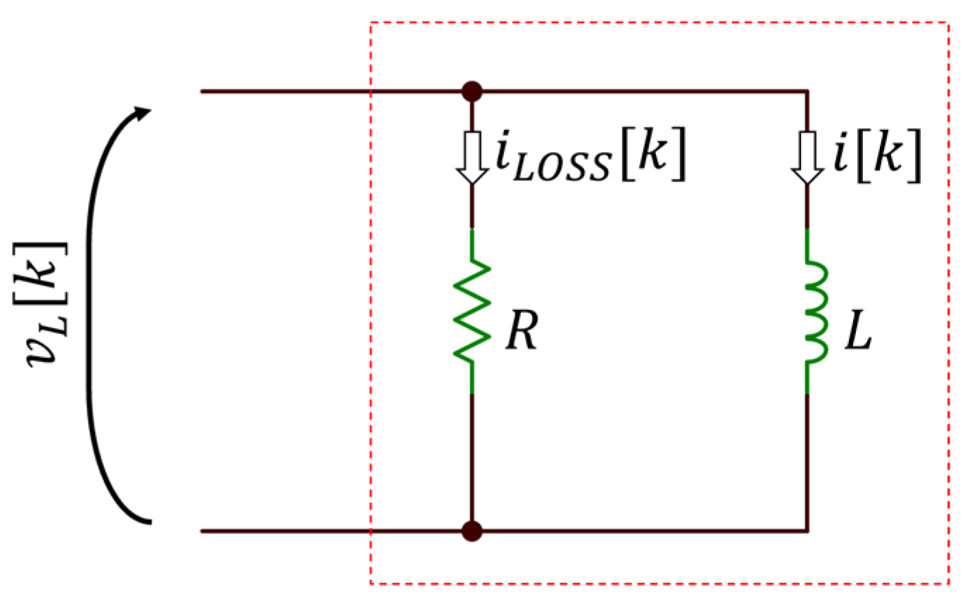
4.3. Lossy Magnetic Hysteresis Cycle Reconstruction

The induction B(t) computed by iGSE and TDNU is in phase with the inductor current I (t). According to Lenz law, the inductor voltage $v_L\left(t\right)$ is in quadrature with the current, resulting in a null average power loss. This means that the B-H trajectory would present no hysteresis. This is in conflict with the actual losses that are estimated by the two methodologies. To resolve this conflict, an additional artificial current term $i_{LOSS}$, in phase with the inductor voltage, must be considered. This term can be determined assuming an equivalent R-L parallel circuit model such as the one shown in Figure 7.

In this circuit, the inductor is ideal, and the instantaneous power related to the core losses is absorbed by the resistive element. Expressing the quantities in a time-discrete domain, a loss current i_LOSS[k] can be computed by the ratio between the computed losses p[k] and the instantaneous voltage across the inductor v_L[k]. The latter can be computed from the numerical expression of the Lentz law. Although the magnetic field H is not measured in this setup, it is possible to assume that, together with the induction B, it should accommodate the instantaneous value of the losses.

$$v_L[k]=N{S}_t\frac{B[k]-B[k-1]}{t[k]-t[k-1]}$$

(12)

$$i_{LOSS}[k]=\frac{p[k]}{v_L[k]}$$

(13)

where S_t is the cross-section of the toroid. From the loss current, the loss-affected H field can is derived as

$$H[k]=(i_{LOSS}[k]+i[k])\frac{N}{\lambda }$$

(14)

where λ is the magnetic path length of the toroid core.

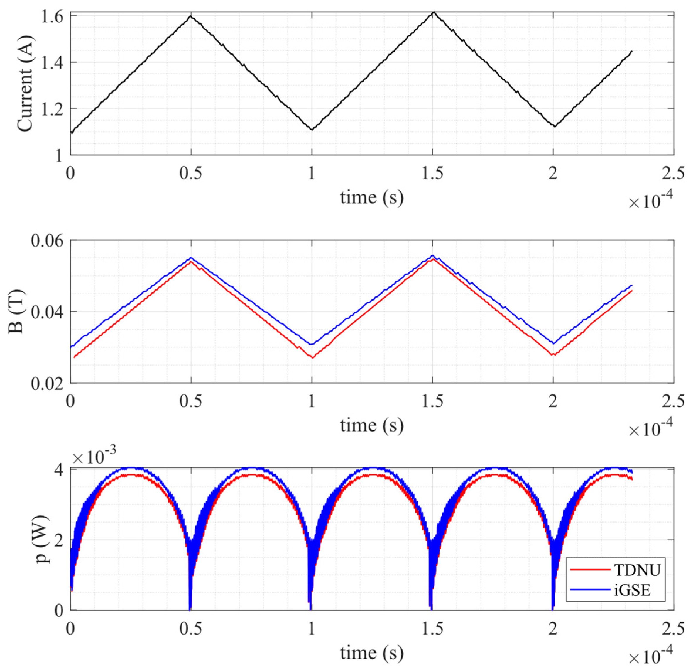
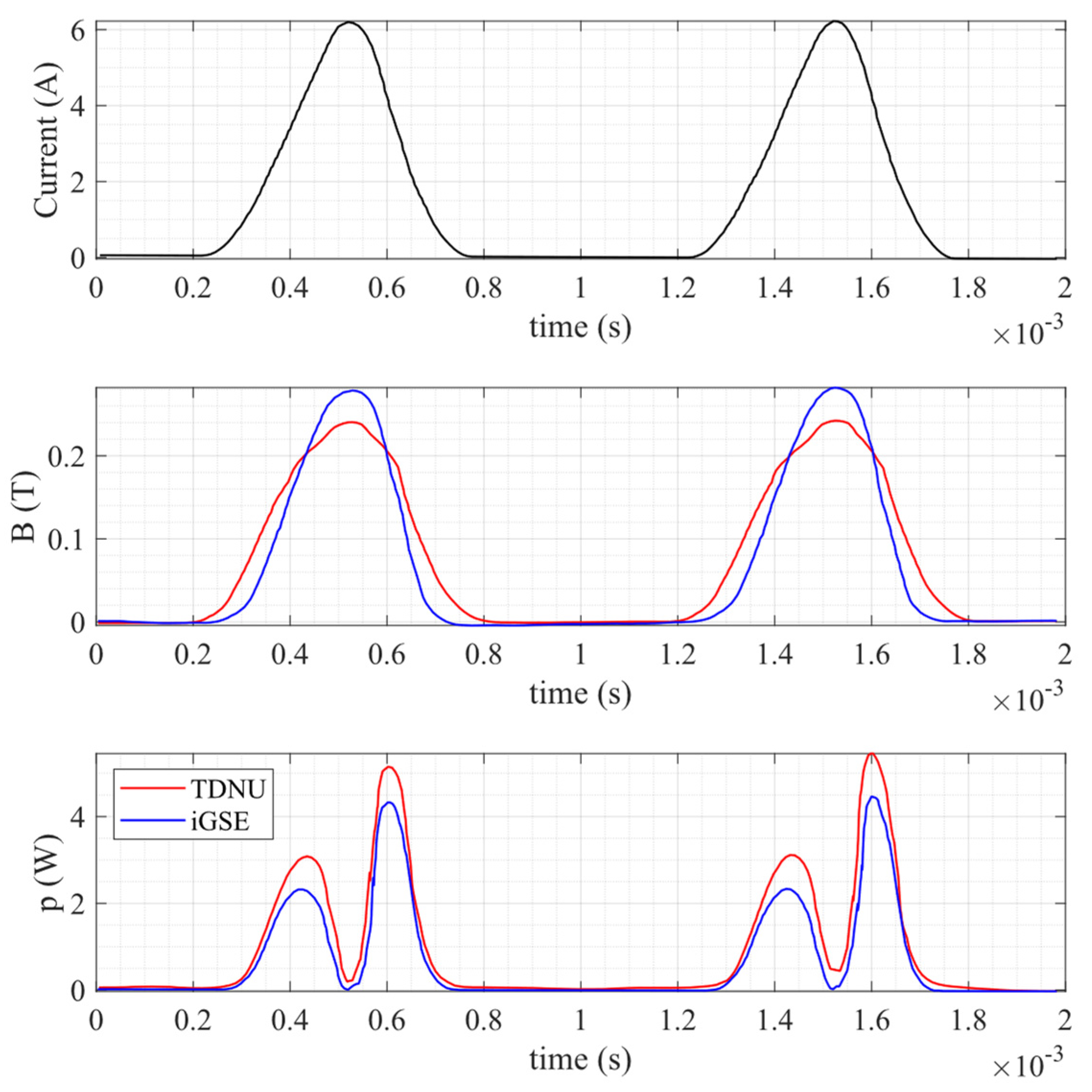
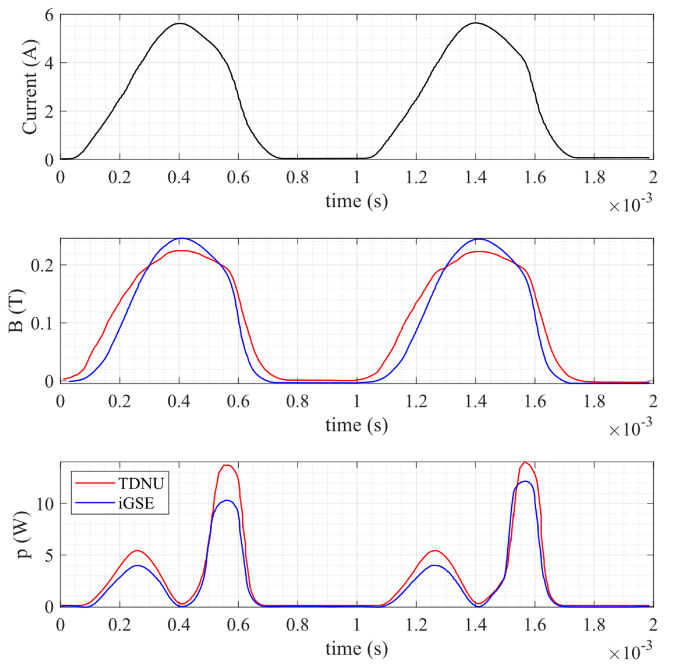
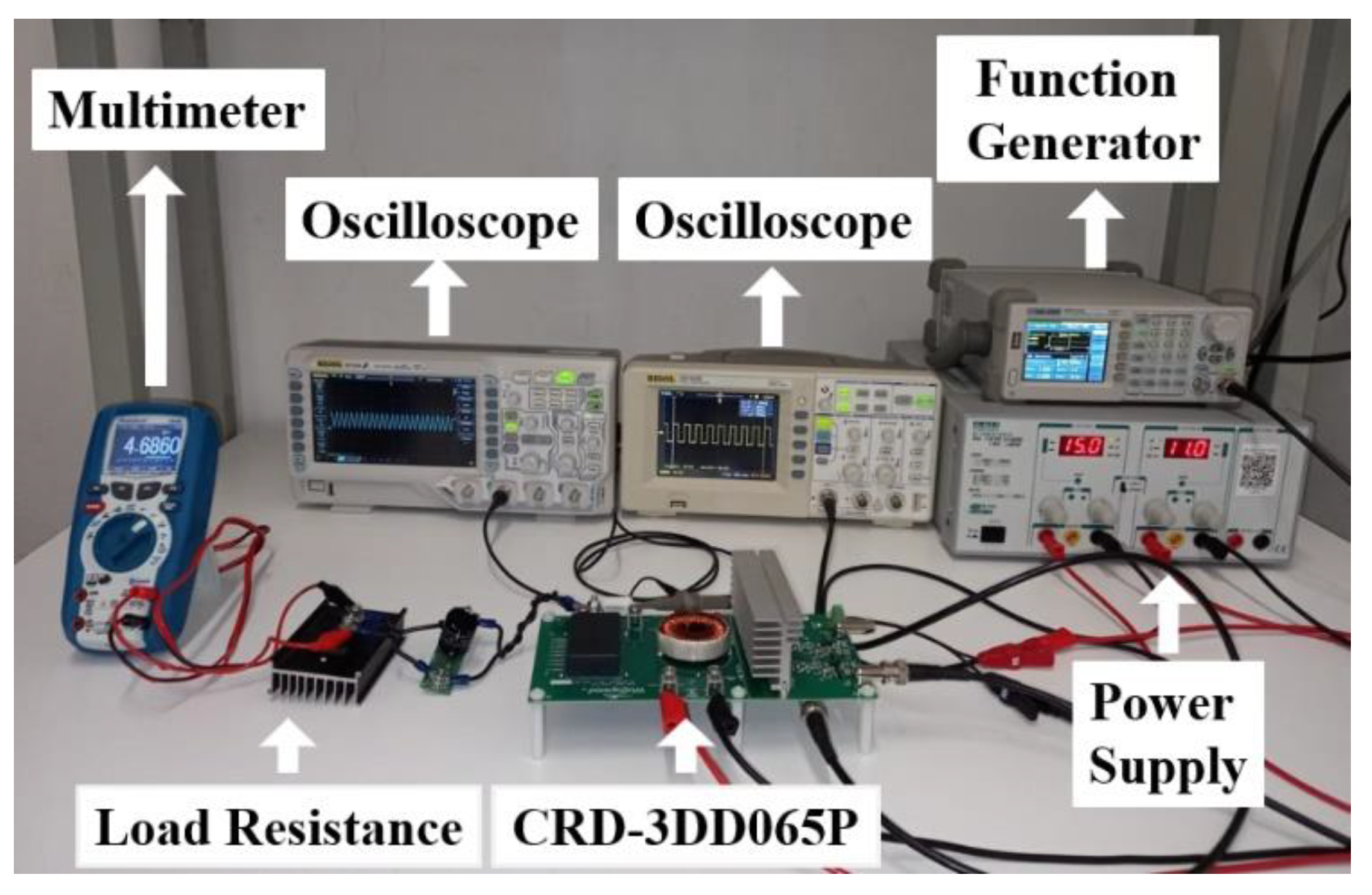
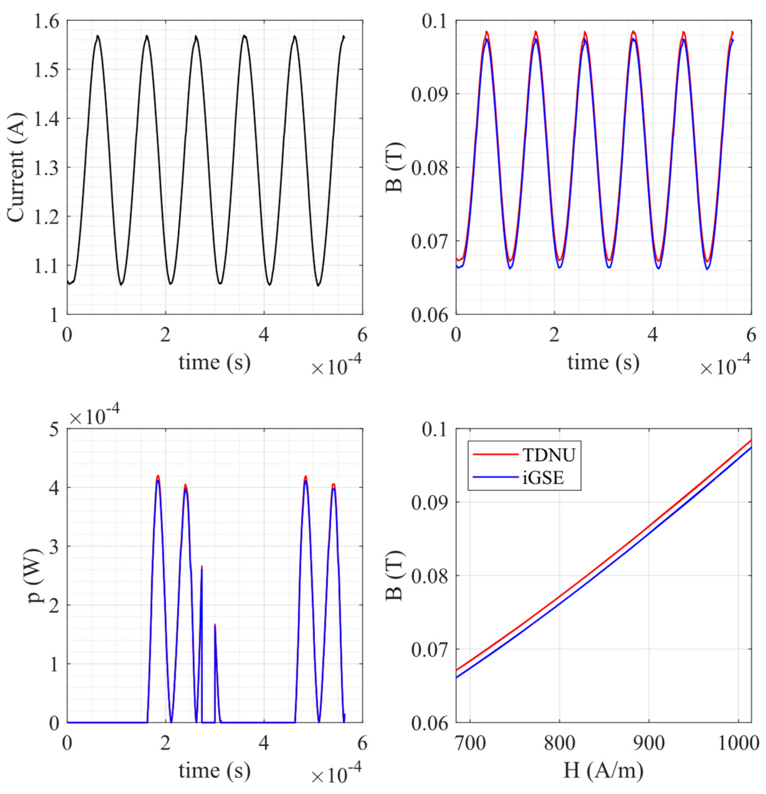
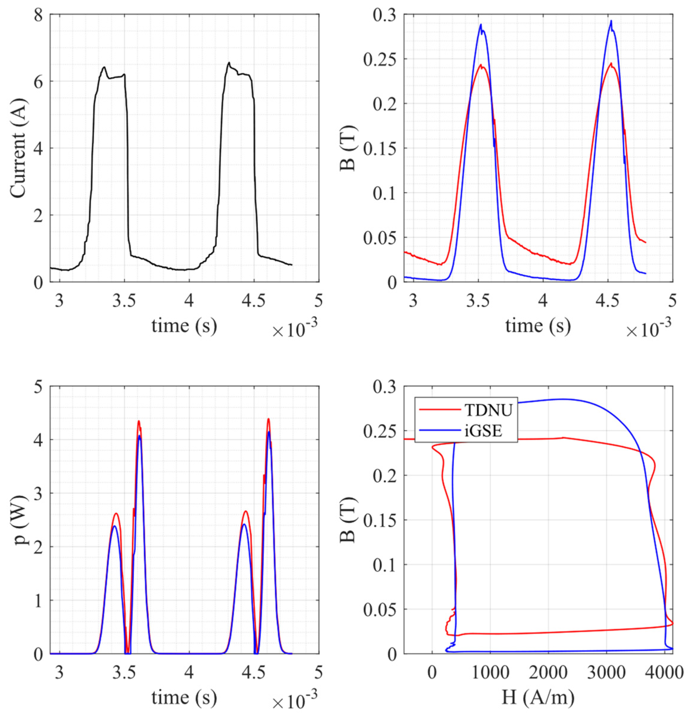
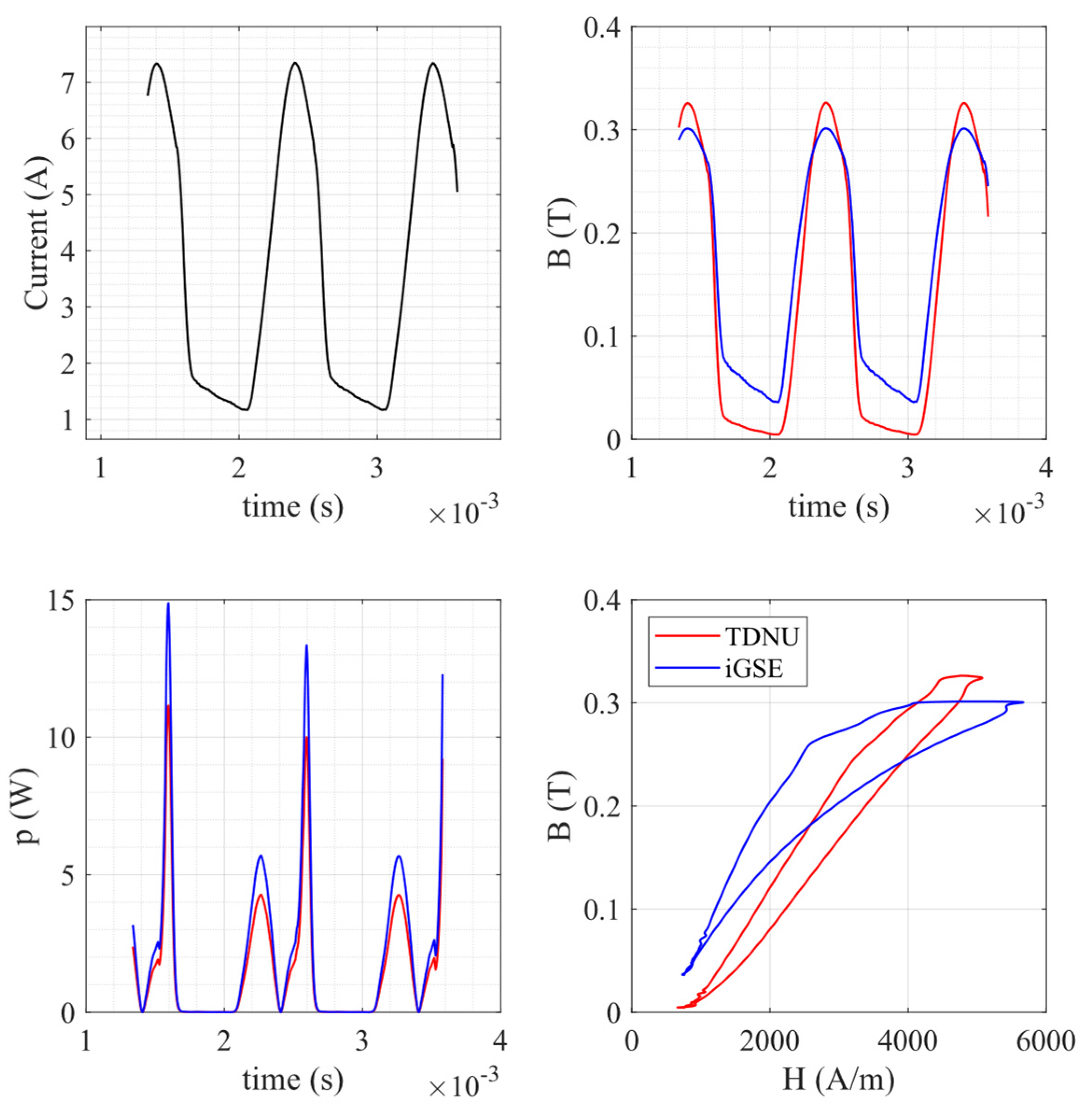
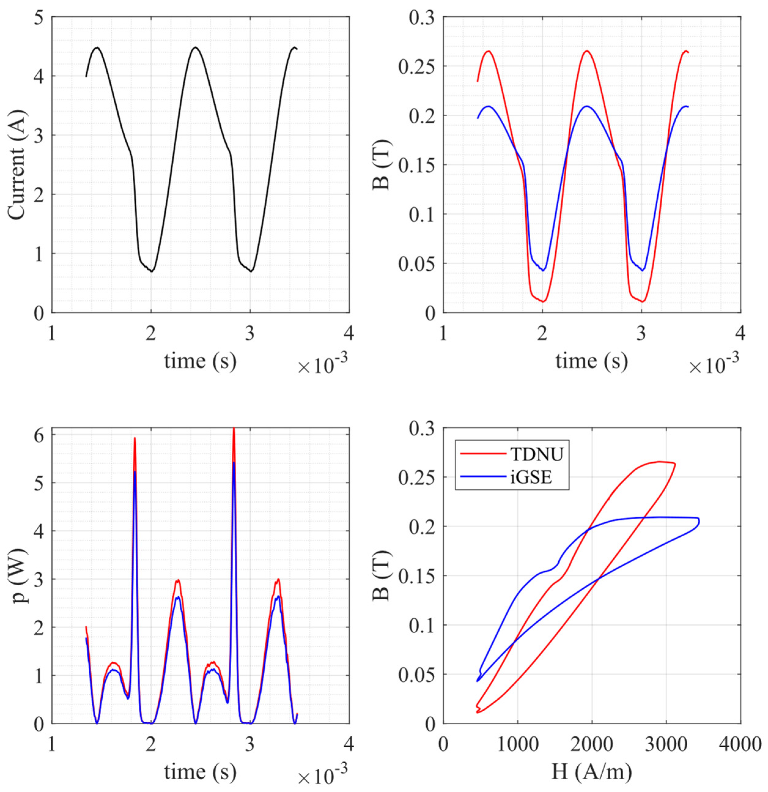
5. Measurements and Simulation Results

The proposed methodology is validated, both in experimental and simulated environment, through a series of different tests, aimed at assessing the consistency of the three techniques. In the first test, the inductor current used for the different loss estimation methodologies is acquired from an LTSpice simulation. In the second test, the inductor current is measured on the real DC-DC Buck converter. For both tests, the four operating conditions described in

Table 4. Case studies operating conditions.

Case	Frequency fs	Load Resistance RL	Duty Cycle D
I	10 kHz	10 Ω	0.5
II	1 kHz	10 Ω	0.3
III	1 kHz	10 Ω	0.5
IV	1 kHz	10 Ω	0.8

are considered to explore different current waveforms of the inductor. These operating conditions allow to compare the core loss estimation under significative different operating conditions, considering both the CCM and DCM case. For each operating condition:

• The RMS losses are computed with three methodologies (SE, iGSE, TDNU);
• The instantaneous losses are computed with two methodologies (iGSE, TDNU);
• For the experimental data, the lossy B-H curve is reconstructed with two methodologies (iGSE, TDNU).

The DC-DC converter circuit model simulated by using LTSpice is shown in Figure 7. Simulations were performed as transient analysis with a minimum timestep of 10 ns to capture the high frequency non-linear dynamics of the switching components. For the same reason, parasitic inductances were added on the MOSFET, diode and output capacitor. The small timestep allowed a detailed reconstruction of the inductor current waveform, which is a critical aspect, because the current is directly related to B as shown in Figure 8, and the B is numerically differentiated, as shown in Figure 4, to compute the instantaneous power loss.

In Figure 9, Figure 10, Figure 11 and Figure 12, the waveforms related to the Buck DC-DC converter operating in Case I, II, III and IV are shown, respectively. Each figure represents the inductor current, the instantaneous magnetic induction and the instantaneous losses.

Different measurements at different operating frequencies and duty cycles were performed and the test parameters are shown in Table 4. The converter input voltage was fixed to V_i = 30 V, to reproduce conditions analogous to those used in the simulation test. Figure 13 shows the experimental setup used to measure the inductor current.

In Figure 14, Figure 15, Figure 16 and Figure 17, the waveforms relative to the Buck DC-DC converter operating in Case I, II, III and IV are shown, respectively. Each figure represents the inductor current, the instantaneous magnetic induction field, the instantaneous losses, and the reconstructed lossy B-H profiles. In

Table 5. Core losses in the four operating conditions for experimental inductor currents.

Case	SE	iGSE	TDNU
I	2.40 mW	2.63 mW	2.64 mW
II	0.65 W	0.63 W	0.73 W
III	0.58 W	0.51 W	0.62 W
IV	2.40 W	2.63 W	2.64 W

, the average losses for the four cases are compared between the methodologies. All the measured current waveforms are very close to the results predicted by the numerical simulations. The greatest difference between the simulated and measured data is for the Case I. This is mainly due to the highest operating frequency which increases the effect of the parasitic components. However, as shown in Table 5, the estimated core losses are consistent with those derived from the simulations. This leads to the conclusion that, even if the current waveforms might exhibit some differences, the computed core losses are not very sensible to these variations.

Table 6. Core losses in the four operating conditions for simulated inductor currents.

Case	SE	iGSE	TDNU
I	2.36 mW	2.53 mW	2.58 mW
II	0.59 W	0.61 W	0.71 W
III	0.54 W	0.49 W	0.60 W
IV	1.03 W	1.06 W	1.10 W

shows the average losses determined by using the current computed through simulation for the considered cases and methodologies. Table 6 shows the core losses derived by using the experimentally measured currents. The comparison is discussed in the conclusion section.

6. Conclusions

In this paper, a novel methodology for core losses estimation was compared against two state-of-the-art approaches in the study of a DC-DC power converter. Core loss estimation in time-domain is difficult due to non-linear, dynamic and geometrical phenomena involving the magnetic material. Moreover, practical applications such as power converters usually involve non-sinusoidal excitations which further complicates the study. A unidirectional topology has been considered. The proposed methodology and the two comparison methodologies allowed the estimation of the core losses in the inductor of a DC-DC Buck converter by considering detailed magnetic behavior of the core. The obtained results showed that the TDNU methodology results in a core losses estimation comparable with the other methods, yet the estimations are usually slightly higher than others resulting from the compared methods, thanks to the ability of the TDNU to consider the field non-uniform distribution inside the core.

The proposed accurate core loss model leads to the possibility of including a real induction model inside the SPICE environment. This model is able to exhibit a consistent behavior considering core non-linearities. In fact, since the TDNU method is inherently a time-domain approach and is natively implemented in the form of a Spice circuit, it is a promising candidate to be included in larger circuit designs and can benefit from the optimized integration engines coupled with circuit simulation software.

References

1. Castellazzi, A.; Gurpinar, E.; Wang, Z.; Suliman Hussein, A.; Garcia Fernandez, P. Impact of Wide-Bandgap Technology on Renewable Energy and Smart-Grid Power Conversion Applications Including Storage. Energies 2019, 12, 4462. [Google Scholar] [CrossRef] [Green Version]
2. Millan, J.; Godignon, P.; Perpiñà, X.; Perez-Tomas, A.; Rebollo, J. A Survey of Wide Bandgap Power Semiconductor Devices. IEEE Trans. Power Electron. 2014, 29, 2155–2163. [Google Scholar] [CrossRef]
3. Loncarski, J.; Monopoli, V.G.; Leuzzi, R.; Ristic, L.; Cupertino, F. Analytical and Simulation Fair Comparison of Three Level Si IGBT Based NPC Topologies and Two Level SiC MOSFET Based Topology for High Speed Drives. Energies 2019, 12, 4571. [Google Scholar] [CrossRef] [Green Version]
4. Kolar, J.W.; Bortis, D.; Neumayr, D. The ideal switch is not enough. In Proceedings of the 2016 28th International Symposium on Power Semiconductor Devices and ICs (ISPSD), Prague, Czech Republic, 12–16 June 2016; pp. 15–22. [Google Scholar]
5. Detka, K.; Górecki, K.; Grzejszczak, P.; Barlik, R. Modeling and Measurements of Properties of Coupled Inductors. Energies 2021, 14, 4088. [Google Scholar] [CrossRef]
6. Musumeci, S.; Solimene, L.; Ragusa, C. Identification of DC Thermal Steady-State Differential Inductance of Ferrite Power Inductors. Energies 2021, 14, 3854. [Google Scholar] [CrossRef]
7. Salinas, G.; Serrano-Vargas, J.; Muñoz-Antón, J.; Alou, P. Thermal Resistance Matrix Extraction from Finite-Element Analysis for High-Frequency Magnetic Components. Energies 2021, 14, 3075. [Google Scholar] [CrossRef]
8. Mazgaj, W.; Sierzega, M.; Szular, Z. Approximation of Hysteresis Changes in Electrical Steel Sheets. Energies 2021, 14, 4110. [Google Scholar] [CrossRef]
9. TDK. EPCOS Data Book 2013. Ferrites and Accessories. Available online: https://www.tdk-electronics.tdk.com/download/519704/069c210d0363d7b4682d9ff22c2ba503/ferrites-and-accessories-db-130501.pdf (accessed on 9 October 2021).
10. Salas, R.A.; Pleite, J. Equivalent Electrical Model of a Ferrite Core Inductor Excited by a Square Waveform Including Saturation and Power Losses for Circuit Simulation. IEEE Trans. Magn. 2013, 49, 4257–4260. [Google Scholar] [CrossRef]
11. Corti, F.; Grasso, F.; Paolucci, L.; Pugi, L.; Luchetti, L. Circular Coil for EV Wireless Charging Design and Optimization Considering Ferrite Saturation. In Proceedings of the 5th IEEE International Forum on Research and Technologies for Society and Industry (RTSI), Florence, Italy, 9–12 September 2019; pp. 279–284. [Google Scholar] [CrossRef] [Green Version]
12. Locorotondo, E.; Pugi, L.; Corti, F.; Becchi, L.; Grasso, F. Analytical Model of Power MOSFET Switching Losses due to Parasitic Components. In Proceedings of the 2019 IEEE 5th International forum on Research and Technology for Society and Industry (RTSI), Florence, Italy, 9–12 September 2019; pp. 331–336. [Google Scholar]
13. Grasso, F.; Luchetta, A.; Manetti, S.; Piccirilli, M.C. Symbolic techniques in neural network based fault diagnosis of analog circuits. In Proceedings of the 2010 XIth International Workshop on Symbolic and Numerical Methods, Modeling and Applications to Circuit Design (SM2ACD), Gammarth, Tunisia, 4–6 October 2010; pp. 1–4. [Google Scholar]
14. Papamanolis, P.; Guillod, T.; Krismer, F.; Kolar, J.W. Minimum Loss Operation and Optimal Design of High-Frequency Inductors for Defined Core and Litz Wire. IEEE Open J. Power Electron. 2020, 1, 469–487. [Google Scholar] [CrossRef]
15. Guillod, T.; Papamanolis, P.; Kolar, J.W. Artificial Neural Network (ANN) Based Fast and Accurate Inductor Modeling and Design. IEEE Open J. Power Electron. 2020, 1, 284–299. [Google Scholar] [CrossRef]
16. Vidal, N.; Lopez-Villegas, J.M.; Del Alamo, J.A. Analysis and Optimization of Multi-Winding Toroidal Inductors for Use in Multilayered Technologies. IEEE Access 2019, 7, 93537–93544. [Google Scholar] [CrossRef]
17. Salvini, A.; Fulginei, F.R.; Coltelli, C. A neuro-genetic and time-frequency approach to macromodeling dynamic hysteresis in the harmonic regime. IEEE Trans. Magn. 2003, 39, 1401–1404. [Google Scholar] [CrossRef]
18. Herceg, D.; Chwastek, K.; Herceg, Đ. The Use of Hypergeometric Functions in Hysteresis Modeling. Energies 2020, 13, 6500. [Google Scholar] [CrossRef]
19. Kovacevic, I.F.; Friedli, T.; Musing, A.M.; Kolar, J.W. Full PEEC Modeling of EMI Filter Inductors in the Frequency Domain. IEEE Trans. Magn. 2013, 49, 5248–5256. [Google Scholar] [CrossRef]
20. Saeed, S.; Georgious, R.; Garcia, J. Modeling of Magnetic Elements Including Losses—Application to Variable Inductor. Energies 2020, 13, 1865. [Google Scholar] [CrossRef] [Green Version]
21. Mu, M.; Zheng, F.; Li, Q.; Lee, F.C. Finite element analysis of inductor core loss under DC bias conditions. IEEE Trans. Power Electron. 2013, 28, 4414–4421. [Google Scholar] [CrossRef]
22. Lin, D.; Zhou, P.; Fu, W.; Badics, Z.; Cendes, Z. A Dynamic Core Loss Model for Soft Ferromagnetic and Power Ferrite Materials in Transient Finite Element Analysis. IEEE Trans. Magn. 2004, 40, 1318–1321. [Google Scholar] [CrossRef]
23. Cui, H.; Ngo, K.D.T. Transient Core-Loss Simulation for Ferrites With Nonuniform Field in SPICE. IEEE Trans. Power Electron. 2018, 34, 659–667. [Google Scholar] [CrossRef]
24. Corti, F.; Reatti, A.; Cardelli, E.; Faba, A.; Rimal, H.P. Improved Spice Simulation of Dynamic Core Losses for Ferrites With Nonuniform Field and Its Experimental Validation. IEEE Trans. Ind. Electron. 2021, 68, 12069–12078. [Google Scholar] [CrossRef]
25. Steinmetz, C.P. On the law of hysteresis. Proc. IEEE 1984, 72, 197–221. [Google Scholar] [CrossRef]
26. Antonio, S.Q.; Faba, A.; Rimal, H.P.; Cardelli, E. On the Analysis of the Dynamic Energy Losses in NGO Electrical Steels under Non-Sinusoidal Polarization Waveforms. IEEE Trans. Magn. 2020, 56, 6300115. [Google Scholar]
27. Antonio, S.Q.; Lozito, G.M.; Ghanim, A.M.; Laudani, A.; Rimal, H.; Faba, A.; Chilosi, F.; Cardelli, E. Analytical formulation to estimate the dynamic energy loss in electrical steels: Effectiveness and limitations. Phys. B Condens. Matter 2020, 579, 411899. [Google Scholar] [CrossRef]
28. Lee, J.-I.; Shin, K.-H.; Bang, T.-K.; Kim, K.-H.; Hong, K.-Y.; Choi, J.-Y. Core-Loss Analysis of Linear Magnetic Gears Using the Analytical Method. Energies 2021, 14, 2905. [Google Scholar] [CrossRef]
29. Venkatachalam, K.; Sullivan, C.R.; Abdallah, T.; Tacca, H. Accurate prediction of ferrite core loss with nonsinusoidal waveforms using only Steinmetz parameters. In Proceedings of the 2002 IEEE Workshop on Computers in Power Electronics, Mayaguez, PR, USA, 3–4 June 2002; pp. 36–41. [Google Scholar] [CrossRef] [Green Version]
30. Rimal, H.P.; Ghanim, A.M.; Antonio, S.Q.; Lozito, G.M.; Faba, A.; Cardelli, E. Modelling of dynamic losses in soft ferrite cores. Phys. B Condens. Matter 2020, 579, 411811. [Google Scholar] [CrossRef]
31. Wolfspeed. Kit-CRD-3DD065P. Available online: https://www.wolfspeed.com/kit-crd-3dd065p (accessed on 9 October 2021).
32. Mag-Inc. Powder Cores. Kool-Mu Cores. Available online: https://www.mag-inc.com/Products/Powder-Cores/Kool-Mu-Cores/Kool-Mu-Material-Curves (accessed on 9 October 2021).
Figure 1. LTSpice circuit for Time-Domain Core Loss estimation based on wipe out rule [24]. The red dotted box includes the equivalent lumped circuit of the DC-DC converter. The blocks used for the real time core loss estimation are shown inside the blue box.
Energies 14 06498 g001
Figure 2. Buck converter unidirectional topology.
Energies 14 06498 g002
Figure 3. Magnetic characteristics of the toroidal core. (a) BH curve and permeability. (b) Magnetic permeability curve.
Energies 14 06498 g003
Figure 4. Core loss estimation using classical Steinmetz Equations.
Energies 14 06498 g004
Figure 5. Core loss estimation using iGSE.
Energies 14 06498 g005
Figure 6. Core loss estimation using non-uniform magnetic field density.
Energies 14 06498 g006
Figure 7. Equivalent lossy circuit model for H-B reconstruction.
Energies 14 06498 g007
Figure 8. LTSpice simulation for the acquisition of the inductor current waveforms in different operating conditions of the power converter.
Energies 14 06498 g008
Figure 9. Simulated DC-DC waveforms for Case I (f = 10 kHz D = 0.5): Inductor current, instantaneous magnetic induction B, instantaneous losses p. Red and blue traces are the waveforms relative to the TDNU and iGSE estimation methods, respectively.
Energies 14 06498 g009
Figure 10. Simulated DC-DC waveforms for Case II (f = 1 kHz D = 0.3): Inductor current, instantaneous magnetic induction B, instantaneous losses p. Red and blue traces are the waveforms relative to the TDNU and iGSE estimation methods, respectively.
Energies 14 06498 g010
Figure 11. Simulated DC-DC waveforms for Case III (f = 1 kHz D = 0.5): Inductor current, instantaneous magnetic induction B, instantaneous losses p. Red and blue traces are the waveforms relative to the TDNU and iGSE estimation methods, respectively.
Energies 14 06498 g011
Figure 12. Simulated DC-DC waveforms for Case IV (f = 1 kHz D = 0.8): Inductor current, instantaneous magnetic induction B, instantaneous losses p. Red and blue traces are the waveforms relative to the TDNU and iGSE estimation methods, respectively.
Energies 14 06498 g012
Figure 13. Experimental setup.
Energies 14 06498 g013
Figure 14. DC-DC waveforms for Case I (f = 10 kHz D = 0.5): Inductor current, instantaneous magnetic induction B, instantaneous losses p, reconstructed hysteresis loop. Red and blue traces are the waveforms relative to the TDNU and iGSE estimation methods, respectively.
Energies 14 06498 g014
Figure 15. DC-DC waveforms for Case II (f = 1 kHz D = 0.3): Inductor current, instantaneous magnetic induction B, instantaneous losses p, reconstructed hysteresis loop. Red and blue traces are the waveforms relative to the TDNU and iGSE estimation methods, respectively.
Energies 14 06498 g015
Figure 16. DC-DC waveforms for Case III (f = 1 kHz D = 0.5): Inductor current, instantaneous magnetic induction B, instantaneous losses p, reconstructed hysteresis loop. Red and blue traces are the waveforms relative to the TDNU and iGSE estimation methods, respectively.
Energies 14 06498 g016
Figure 17. DC-DC waveforms for Case IV (f = 1 kHz D = 0.8): Inductor current, instantaneous magnetic induction B, instantaneous losses p, reconstructed hysteresis loop. Red and blue traces are the waveforms relative to the TDNU and iGSE estimation methods, respectively.
Energies 14 06498 g017