Abstract
The quality of feedstock used in base oil processing depends on the source of the crude oil. Moreover, the refinery is fed with various blends of crude oil to meet the demand of the refining products. These circumstances have caused changes of quality of the feedstock for the base oil production. Often the feedstock properties deviate from the original properties measured during the process design phase. To recalculate and remodel using first principal approaches requires significant costs due to the detailed material characterizations and several pilot-plant runs requirements. To perform all material characterization and pilot plant runs every time the refinery receives a different blend of crude oil will simply multiply the costs. Due to economic reasons, only selected lab characterizations are performed, and the base oil processing plant is operated reactively based on the feedback of the lab analysis of the base oil product. However, this reactive method leads to loss in production for several hours because of the residence time as well as time required to perform the lab analysis. Hence in this paper, an alternative method is studied to minimize the production loss by reacting proactively utilizing machine learning algorithms. Support Vector Regression (SVR), Decision Tree Regression (DTR), Random Forest Regression (RFR) and Extreme Gradient Boosting (XGBoost) models are developed and studied using historical data of the plant to predict the base oil product kinematic viscosity and viscosity index based on the feedstock qualities and the process operating conditions. The XGBoost model shows the most optimal and consistent performance during validation and a 6.5 months plant testing period. Subsequent deployment at our plant facility and product recovery analysis have shown that the prediction model has facilitated in reducing the production recovery period during product transition by 40%.
1. Introduction
Lubricants are important fluids and are commonly used to suppress friction between two metallic surfaces and as a medium for heat transportation. These base oils are obtained from various sources such as petroleum raffinates, bio-based oils, olefins and plastic wastes, with some additives to enhance their properties. A few examples of processes used to produce the base oils are solvent extraction, severe hydrocracking, olefin polymerization and esterification.
This paper focuses on a severe hydrocracking process in our facility that involves three series of reactions which are hydrotreating, hydroisomerisation and hydrodearomatisation. The feedstock used is originated from the waxy raffinate obtained from crude oil atmospheric distillation. This waxy raffinate is then distilled at vacuum condition to obtain three different grades with the final product kinematic viscosities of 4 cSt, 6 cSt and 10 cSt ranges. In the hydrotreating process, feedstock is fed into the hydrotreating reactor to reduce the sulfur and nitrogen content to an acceptable level. The hydrotreating reactor also cracks the naphthene rings which will improve the viscosity index of the base oil product. The product from this reaction then undergoes the hydroisomerization reaction, where the base oil molecules are isomerized to lower its pour point. Next, the product undergoes the hydrodearomatization process to increase the base oil product oxidative stability. Finally, the product is distilled at vacuum condition to remove the lighter materials. Figure 1 shows a simplified flow diagram of the base oil processing plant.
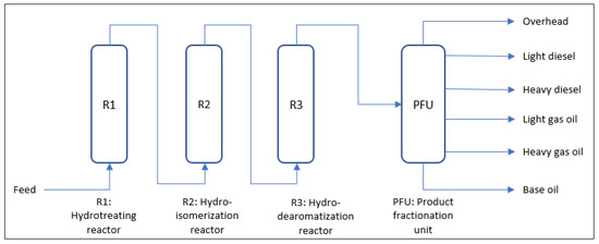
Figure 1.
Simplified process flow diagram of the base oil processing plant.
In the hydrotreating reactor, the sulfur and nitrogen contents are reduced to a very low level with the right combination of catalyst, temperature and appropriate hydrogen partial pressures. The ease of desulfurization depends on the type of carbon–sulfur bonds present in the feedstock [1,2]. Groups of alkyl sulfides and polysulfides possess weaker carbon–sulfur bonds, which makes for easier sulfur removal. On the other hand, the sulfur that comes from thiophene and aromatics are more difficult to be removed, requiring higher temperature [2,3]. Meanwhile the nitrogen contents commonly comes in the form of pyrrole and pyridine derivatives [2,4]. The initial step of the nitrogen removal is pressure dependent as it is close to the equilibria [2,4], yet very high temperatures can reduce the nitrogen removal rate [2,5]. Therefore, controlling the temperature and pressure balance is highly important for the sulfur and nitrogen removal process.
In the hydroisomerization process, n-paraffin in the feed reacts with zeolite catalysts and are selectively cracked and isomerized under a hydrogen-rich environment. Through this hydroisomerization process, the pour point of the base oil product is reduced. At the same time, the aromatic content in both feedstock and the product are a critical parameter in base oil processing. Aromatics cause oxidative instability in the product, as well as lower the viscosity index [2]. The lower the aromatic content, the more stable the final product is over time. Therefore, the hydrodearomatization reaction is needed to remove the remaining aromatics in the base oil product. The temperature and pressure condition of the hydrodearomatization reactor is critical, as the limiting factor of hydrodearomatization activity over sulfide metal oxide catalyst is the thermodynamic equilibrium [2].
Apart from the operating conditions, such as temperature and pressure, the feed properties are equally important in predicting the base oil product properties. The nature of the feed, primarily the heavy parts of the crude oil, is made up of various chemical groups such as paraffins, aromatics, sulfur and nitrogen-containing compounds. The heavy hydrocarbons can have numerous possibilities of molecular structures, to the point where obtaining the exact composition of the molecules is not a feasible task [6]. Thus, the process is very difficult to model for all combinations of reactions and feed properties using a first principal approach. Furthermore, in practice only certain lab analyses are performed at non-rapid frequencies, solely to indicate the bulk properties of the feedstock in general. The feedstock lab analysis performed are simulated distillation, sulfur content, nitrogen content, aromatics content, wax content, viscosity, dewaxed oil viscosity, dewaxed oil viscosity index and density. In addition, the necessary pilot plant runs require days of operation to develop even the first principal model. Further iterations of these detailed studies carry a cumulative monetary and time cost. With these costs in mind, the plant currently runs reactively based on lab analysis of the base oil product, using the reported product specification to guide in further decision making. If the product is under or over the specification, the plant operator will adjust the operating condition accordingly. This reactive mode of operation possesses its own weakness in that during situations where product results are uncertain, the product must be diverted to a slopping tank. As the proper results are being waited upon, which can take several hours, there is loss of production in this period.
This presents a motivation for the authors to explore other ways to improve production. Recently, the rise of several machine learning algorithms, which are readily available at zero cost, provides an interesting and promising alternative for solving prediction problems. These machine learning capabilities have grown substantially as computing capabilities become more advanced and accessible. Through utilization of the readily available plant historical data, machine learning has the potential to reduce the time consumed and costs expended for these laboratory tests [7], and deliver a prediction of its own either for use as a secondary reference or as an accurate black-box representation of the laboratory analysis. Recent studies on modeling viscosity prediction using low field nuclear magnetic resonance also highlighted the need for data driven approaches due to the complexity of the viscometry behavior of hydrocarbon mixtures, especially within the petroleum industry [8]. In this paper, Support Vector Regression (SVR), Decision Tree Regression (DTR), Random Forest Regression (RFR) and Extreme Gradient Boosting (XGBoost) machine learning models are developed using historical data of the plant to predict the base oil product kinematic viscosity and viscosity index based on the feedstock qualities and the process operating conditions. Subsequent plant deployment at our facility and product recovery analysis by using the final selected machine learning model are also presented to highlight the key benefits.
This paper is presented as follows: Section 2 provides some theoretical background of the machine learning models considered in this paper. Section 3 discusses the dataset used and the methodology adopted. Section 4 presents the modelling results and the corresponding plant testing and deployment at our facility. Finally, Section 5 concludes the study and findings.
2. Machine Learning Models
In this paper, four types of the machine learning algorithms are studied, namely, Support Vector Regression (SVR), Decision Tree Regression (DTR), Random Forest Regression (RFR) and Extreme Gradient Boosting (XGBoost). SVR was developed by Vladimir N. Vapnik in the statistical learning Vapnik–Chervonenkis (VC) theory. SVR is positioned to generalize on yet-to-be seen data [9]. SVR formulates regression as convex optimization problems [10,11]. The goal is to find the optimum distance of the support vectors from the prediction function or known as tube width [9,10]. The support vector algorithm will define the hyperplanes such that:
The prediction function is the median, between the and hyperplanes as illustrated in Figure 2. The and also known as tube with the width of [10]. The points that lie on and are the support vectors. Hence to find the best fit is by defining the ε-insensitive loss function as (3) [10].
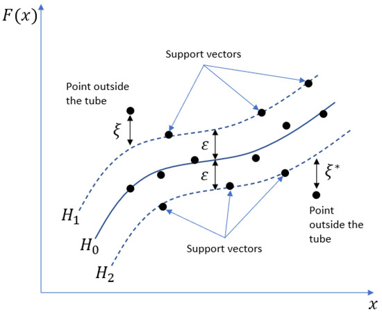
Figure 2.
Illustration of support vector regression, original diagram shown in an article by Drucker H. et al. with permission [10].
The constraint can be defined as in (7) where is defined as (8) and (9).
The width of the hyperplane is the dot product of the difference between vector and and the vector w divided by magnitude of w as in (11). Thus, maximizing the width by maximizing the magnitude of is equivalent to minimizing half of the squared magnitude of (that is convenient for the differentiation). The minimization of the half of the squared magnitude of with the constraint of (4) and (5) is represented in (10). Given the constraints via Lagrange multiplier in the form of Loss function as in (11) whilst and satisfies (14).
Using conditions at and which lead to dual space objective function [10,12] in (12), subject to conditions of (13) and (14).
where is an positive semidefinite matrix, which is equivalent to a kernel function [10,12].
Therefore, the prediction can be written in the form of kernel function as (16). Substituted with kernel radial based function is represented by (17).
For the DTR, the algorithm generates the regression tree by piece-wising the input variable into several ranges and predicts the value based on the average of observed values. Using this piece-wise function, the trees are developed as a graph which begins with one node and branched to many nodes. The topmost node contains the entire dataset, and each subsequent node contains a subset of the dataset. Decision trees have been considered as alternatives to regressions and discriminant analysis [13]. Each range of input variable in the piecewise function has the average observed values as prediction. For illustration, Figure 3 shows the top part of the decision tree for predicting the base oil product kinematic viscosity at 100 °C.
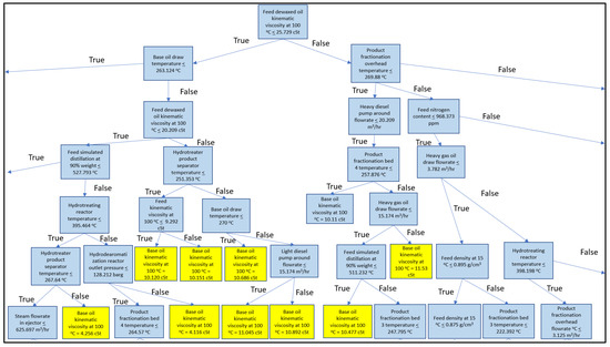
Figure 3.
Example of a portion the decision tree produced in modelling the base oil kinematic viscosity at 100 °C. The blue and yellow color codes denotes the internal nodes and the leaf nodes, respectively. Note that the overall decision tree is much bigger.
The RFR algorithm, on the other hand, is an ensemble learning built from multiple decision trees, resembling a forest. RFR was introduced by Breiman as computing method to handle the nonlinear data [14,15]. Furthermore, the advantage of random forest is that it has the ability to calculate the importance of each input variable which enables it to rank the variables in conformity with their importance [15]. The two important criteria applied in random forest are mean decrease impurity and mean decrease accuracy to order the rank of important variables [12,15]. The mean decrease impurity is calculated based on the sum of the reduction in the impurity node of the categorization on the variables mean over all trees. Mean decrease accuracy is calculated based on the following condition, if a variable is not important, the reuse of its value should not increase the error of the prediction [15]. Out of bag error estimation is used to determine the important variables [14,16]. The Random Forest algorithm will create a number of decision trees and average the outcome from all decision trees as its prediction as illustrated in Figure 4.
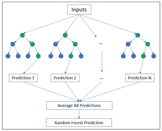
Figure 4.
Illustration of Random Forest as it averages the N predictions from N number of Decisions Trees by Machado G. et al. with permission [17].
XGBoost is a decision tree-based algorithm with an optimized distributed gradient boosting machine learning that is very efficient and flexible [18]. The notion of XGBoost is to use an ensemble of classification or regression trees to fit the samples of training data by minimizing the regularized objective function. It consists of internal nodes and a set of leaf nodes. Based on the boosting method, a series of classifications and regressions are built sequentially. These estimators are associated with the weight to be tuned in the training process so that robust ensemble can be constructed [19,20]. According to Chen and Guestrin the loss function added a function that most improves the model, the loss function simplified at step to (18) [18]:
Define as the instance set of leaf . The loss function can be written by expanding as follows:
For a fixed structure , the optimal weight of leaf by
The corresponding optimal value can be calculated using
Unlike the Random Forest regression, the XGBoost algorithm give scores on every right and wrong prediction and built models from individual learning in an iterative way [18,21].
3. Datasets and Methods
3.1. Base Oil Processing Plant Product Sampling and Laboratory Analysis
An actual base oil product sample is taken at every 8 h interval and used as the target output of the prediction. The properties that are be predicted in this study are the kinematic viscosity measured at 100 °C and the viscosity index. The kinematic viscosity measures the ease of flow of the base oil measured in cSt unit. The higher the viscosity, the lower is its flowability. Meanwhile, the viscosity index measures how the viscosity changes with respect to temperature and it is dimensionless. The kinematic viscosity and viscosity index of the base oil are measured using ASTM D445 and ASTM D5293 standards, respectively [22,23].
3.2. Training, Validation and Plant Testing and Model Deployment Data
Historical data from the base oil processing plant are used in this study. The data are inclusive of feedstock properties, operating conditions and the product properties. As mentioned in Section 1, the critical variables for each reactor unit as well as product distillation units are included. These variables are reactor temperatures, reactor pressures, flow rates, product fractionation pressures, product fractionation draw temperatures, product fractionation draw rates and product fractionation bed temperatures. The feedstock properties that are used are simulated distillation boiling points, viscosity, wax content, dewaxed feed viscosity, dewaxed viscosity index density, sulfur content and nitrogen content. These input variables accumulated to a total of 54 variables. The targeted output parameter are the base oil viscosity and viscosity index.
The historical data contain non-numeric data such as strings whenever there is an error at the transmitter and contains empty data whenever there is unavailability of data especially the low frequency data, such as lab analysis data. Therefore, data pre-processing is performed prior to the machine learning model development. The irrelevant data are removed, missing values are imputed, feature scaling (for SVR) is performed and outliers are removed. When imputing the missing data, the fill forwarding method is used to maintain the continuation of values rather than substituting it with mean value, with the assumption that the value is maintained for a particular period. This is because in practice, the feed tank sampling is performed once prior to feeding to the base oil processing plant and the samplings are taken at the top, middle and bottom of the tank and the values are averaged out. Subsequently whenever the feed tank is switched to another tank, new sampling is performed on the new feed tank.
The dataset is cleaned from outliers by using score method, where z is equal to difference between observed value, and mean of sample, divided by standard deviation, of the sample as in (22). Thus, the row with absolute score value greater than 3 will be considered an outlier and removed from the dataset [24].
Two sets of data from the plant are used as follows:
- Training and validation datasets (for model development)
- ○
- These are data collected from 1 January 2016 to 29 June 2020 consisting of the 54 input variables and 2 output variables (base oil viscosity and viscosity index). The data are split into 70% training data set and 30% validation data set.
- Plant testing and model deployment (for out-of-sample model test)
- ○
- To assess the predictive model performance with the real time data, the models are deployed in a platform application that is connected directly to the plant information system. A testing period is performed from 29 June 2020 until 13 January 2021. The production ran from one product grade continuously for several days and then changed to another grade continuously as per scheduled by the production planner.
The input and the output variables are presented in Table 1.

Table 1.
Inputs and output variables.
3.3. Machine Learning Models Development
3.3.1. Support Vector Regression (SVR) Model Development
The SVR model is trained using the SVR package from scikit-learn library [12]. Radial basis function kernel is used to tackle non-linearity of the base oil process [25]. The hyperparameters C and γ are tuned using grid search cross validation by scikit-learn [12,26,27]. The C parameter is the regularization parameter [12,26] and its values are set to 10−2, 10−1, 100, 101 and 102. Γ is the kernel coefficient for the radial based function [12,26] and its values are set to 10−5, 10−4, 10−6, 10−2, 10−1, 100, 101 and 102. Two kernels are evaluated: radial basis function and linear.
The SVR model is then trained using sets of hyperparameter combinations. All the hyperparameter combinations are tested with 5 splits of cross validation which are evaluated by the R2 score. The hyperparameter combinations are then ranked based on the mean test score of the 5 splits scores. The time taken for each hyperparameter combination calculation is also recorded.
Table 2 shows the top 5 of the rank from 40 different combinations of hyperparameters used in the training of kinematic viscosity using SVR. Average time taken for all the trainings is 0.769 s. The highest mean R2 was 0.992984 and the lowest, RMSE of 0.083759 where the hyperparameters C, γ and kernel are 10, 0.01 and RBF, respectively. Table 3 shows the top 5 of the rank from 40 combinations of hyperparameters used in the training of the viscosity index using SVR. The average time taken for all the trainings is 0.970 s. From the results in both tables, it can be observed that the RBF kernel works well in both kinematic viscosity and viscosity index models development. This is because the base oil process is highly unlikely a linear process as it involves reaction kinetics and equilibriums. The RBF kernel is capable of handling the non-linearity nature of the base oil processing plant behavior.
Table 2.
Top 5 sets of SVR hyperparameters that is used in developing the base oil kinematic viscosity at 100 °C prediction.
Table 3.
Top 5 sets of SVR hyperparameters that used in developing the base oil viscosity index prediction.
C parameter is the regularization parameter as highlighted in (11). Higher C values imply wider width between hyperplanes and which means a larger margin of error; however, it may increase the chance of misclassification. In this study, each model development has shown that the best C value is 10, which is higher than the default value of 1 as given by Scikit Learn [12]. As observed from Table 2 and Table 3, there are two cases where C is equal to 1 resulted in the top 5 ranking (4th rank and 3rd rank in kinematic viscosity and viscosity index model, respectively). This is interesting because it shows the complexity of the base oil process. Although the R2 is high, there are some data points located outside the hyperplanes and possibly due to noises.
From both Table 2 and Table 3, it can also be observed that the optimal value is 0.01 for both kinematic viscosity and viscosity index model development. is the kernel’s coefficient, as shown in (17). The default value of γ given is 0.059. The in this study is moderately lower than the default value indicating that the model is still capable in capturing the behavior and complexity of the data, but at the expense of higher value of C. In term of time consumption, SVR is the second fastest compared to the others.
3.3.2. Decision Tree Regression (DTR) Model Development
For the DTR development, the decision tree is developed using scikit-learn decision tree package [12]. The hyperparameters such as splitter, minimum sample split and minimum samples leaf are varied by using grid search cross validation provided by scikit-learn. In the grid search, two strategies can be implemented for the splitter hyperparameter as provided by the scikit-learn decision tree package: “random” split and “best” split. The minimum number of samples required to split an internal node is set to 2, 3, 4 and 0. The minimum number of samples required to be at a leaf node is set to 1, 2, 3, 4 and 0. For illustration purposes, Figure 3 shows the top part of the decision tree for predicting the base oil product kinematic viscosity at 100 °C.
Table 4 and Table 5 show the top 5 of the rank from 32 different combinations of hyperparameters used in the training of kinematic viscosity and viscosity index models using DTR, respectively. The average time taken for all the trainings is 0.073 s and 0.075 s, respectively. For the kinematic viscosity model, the highest mean R2 is 0.994289 where the hyperparameters minimum samples leaf, minimum samples split and splitter are 4, 2 and random, respectively. On the other hand, the best DTR model for the viscosity index is obtained using the hyperparameters minimum samples leaf, minimum samples split and splitter of 4, 4 and Random, respectively. It can be seen that both kinematic viscosity and viscosity index best models used the random splitter as it has less tendency to overfit. In addition, overfitting is observed for lower number of minimum sample leaf (less than 4). Overall, the DTR models are the fastest to develop compared to the other machine learning models studied in this paper.
Table 4.
Top 5 set of DTR hyperparameters that been used in developing the base oil kinematic viscosity prediction.
Table 5.
Top 5 combination of DTR hyperparameters that been used in developing the base oil viscosity index prediction.
3.3.3. Random Forest Regression (RFR) Model Development
The RFR model development is performed by using random forest regressor package provided by scikit-learn [12]. The number of estimators, minimum sample split, minimum sample leaf and bootstrap hyper parameters are varied by using grid search cross validation by scikit-learn [12]. The number of estimators parameter which indicates the number of trees in the forest are set to 100, 150 and 200. The minimum number of samples required to be split in an internal node is set to 2, 3, 4 and 0. The minimum number of samples required to be at a leaf node is set to 1, 2, 3, 4 and 0. In the grid search, both cases for bootstrap is used, which is enabled (“true”) and disabled (“false”). The Random Forest algorithm creates N number of decision trees and averages the outcome from all decision trees as its prediction as illustrated in Figure 4.
Table 6 shows the top 5 of the rank from 54 combinations of hyperparameters used in the training of viscosity index prediction using RFR. The average time taken for all the trainings is relatively higher compared to the previous two models at 26.084 s. The highest rank is obtained with the hyperparameters bootstrap sampling, and minimum samples leaf, minimum samples split, number of estimators for bootstrap sampling of 2, 4 and 200, respectively. Table 7 shows the corresponding top 5 of the rank from 54 combinations of hyperparameters used in the training of viscosity index prediction using RFR. Average time taken is also high for all the trainings at 26.823 s. The best ranking is given by the hyperparameters bootstrap sampling, and minimum samples leaf, minimum samples split, number of estimators for bootstrap sampling of 1, 2 and 150, respectively.
Table 6.
Top 5 combinations of RFR hyperparameter that been used in developing the base oil kinematic viscosity at 100 °C prediction.
Table 7.
Top 5 combinations of RFR hyperparameter that been used in developing the base oil viscosity index prediction.
3.3.4. Extreme Gradient Boosting (XGBoost) Model Development
The XGBoost model is trained using the XGBoost package provided by PyPl and maintained by Hyunso Cho and team [28]. The hyperparameters (i.e., number of estimator, maximum depth, learning rate and regularization lambda) are tuned using the grid search cross validation by scikit-learn [12]. The number of gradient boosted trees, which is also equivalent to the number of boosting rounds are set to 1000, 1500 and 2000. The maximum depths for base learners are set to 1, 2, 3 and 0. The boosting learning rate are set to 0.1, 0.2, 0.3, 0.4 and 0.5, and the regularization lambda are set to 0.1, 0.5 and 1.0.
Table 8 shows the top 5 of the rank from 180 combinations of hyperparameters used in the training of kinematic viscosity prediction using XGBoost. The average time taken for all the trainings is 26.875 s. The highest mean R2 is 0.996713 with RMSE of 0.0706426 where the learning rate, maximum depth of tree, number of estimators, regularization term lamda are 0.1, 0, 1000 and 0.1, respectively. Table 9 shows the top 5 of the rank from 180 combinations of hyperparameters used in the training of viscosity index prediction using XGBoost. The average time taken for all the trainings is 31.637 s with the best rank obtained with learning rate, maximum depth of tree, number of estimators, and regularization term of 0.1, 0, 2000 and 0.5, respectively.
Table 8.
Top 5 combinations of XGBoost hyperparameter that been used in developing the base oil kinematic viscosity at 100 °C prediction.
Table 9.
Top 5 combinations of XGBoost hyperparameter that been used in developing the base oil viscosity index prediction.
4. Results and Discussion
4.1. Model Training and Validation Performance
The performance of the machine learning algorithms is compared based on their root mean squared error (RMSE), mean absolute error (MAE), mean squared log scale prediction (MSLE), mean absolute percentage error (MAPE), coefficient of determination (R2) and adjusted coefficient of determination (adjusted R2) as presented in Equations (23)–(28). The , , , , and are number of observation, predicted value, observed value, mean observed value, and number of features, respectively [8]. The RMSE is the square root of the average squared difference between the predicted value and observed value whilst MAE is the mean average absolute difference between predicted value and observed value. The difference between RMSE and MAE is that RMSE can be more sensitive to outliers because of the square function [8,29]. The MSLE can be interpreted as a measure of the ratio between the true and predicted values and avoids penalization due to high differences between the viscosity grades and viscosity indexes [8,30]. The MAPE indicates the relative percentages between the sum of errors and provides intuitive interpretation of the prediction as the errors are represented in percentages [8,31].
As mentioned in Section 3.2, these are data collected from 1 January 2016 to 29 June 2020 consisting of the 54 input variables and 2 output variables (base oil viscosity and viscosity index). The data are split into a 70% training data set and a 30% validation data set. It can be observed that in general, the XGBoost showed the best consistency in performance during the training and validation phases for both the kinematic viscosity and viscosity index prediction models. For the kinematic viscosity prediction, the adjusted R2 values are very similar among the machine learning models (approximately ) but the differences are clearly observed in terms of RMSE and MLSE as presented in Table 10. For the viscosity index as presented in Table 11, models developed through XGBoost and SVR show similar performance. In general, the performance of the machine learning models can be ranked as XGBoost > RFR > DTR > SVR for the kinematic viscosity, and XGBoost > SVR > RFR > DTR for the viscosity index output variable.
Table 10.
Kinematic viscosity prediction based on validation dataset performance based on RMSE, MAE, MLSE, R2 and adjusted R2.
Table 11.
Viscosity Index prediction based on validation dataset performance based on RMSE, MAE, MLSE, R2 and adjusted R2.
4.2. Physicochemical Insights from the Machine Learning Activities
One of the advantages of DTR, RFR and XGBoost is the ability to evaluate and produce feature importance. This is very useful for the user because it can tell relative influence of the input variables to the output variable. This enables the operators to prioritize the operating conditions to be changed to meet the desired product target. Figure 5, Figure 6 and Figure 7 show the top 10 relative important factors for kinematic viscosity at 100 °C by DTR, RFR and XGBoost, respectively. The hydrotreating reactor temperature is one of the important input variables as it can impact the product viscosity. At a higher temperature, more molecular cracking will take place, and this will result in a lighter material, hence lowering the product viscosity. The product fractionation parameters such as base oil product flowrate, fractionation bed temperature and pump around flow rate also has a major influence on the base oil viscosity as they determine the purity of the base oil. If the base oil contains too much lighter hydrocarbon, the viscosity will be lower and vice versa. Feature importance analysis also shows that feed properties are significant; for example, the dewaxed feed kinematic viscosity at 100 °C, density, and nitrogen content will impact the process.
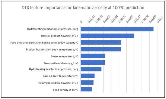
Figure 5.
Top 10 DTR feature importance for kinematic viscosity at 100 °C prediction.
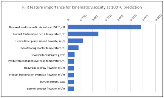
Figure 6.
Top 10 RFR feature importance for kinematic viscosity at 100 °C prediction.
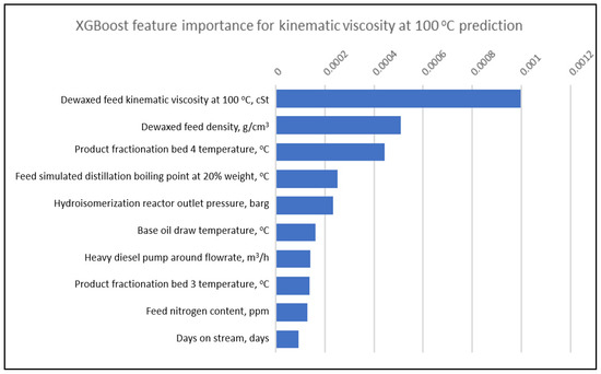
Figure 7.
Top 10 XGBoost feature importance for kinematic viscosity at 100 °C prediction.
The dewaxed feed kinematic viscosity and density is indicative of the feed oil quality, in terms of polyaromatics content in the feed. Higher polyaromatics tends to be more viscous and requires higher hydrotreating reactor temperature hence more cracking took place. Similarly, the higher the feed nitrogen content, the higher the hydrotreating reactor temperature, thus base oil viscosity is lower.
Figure 8, Figure 9 and Figure 10 show the top 10 relative importance for kinematic viscosity at 100 °C by DTR, RFR and XGBoost, respectively. It is observed that the hydrotreating reactor plays a major role in determining the base oil viscosity index. This is because one of the functions of the hydrotreating reactor is to crack the naphthene molecules in the feed, which has a lower viscosity index. Therefore, higher hydrotreating reactor temperatures are required to elevate the final base oil viscosity index.
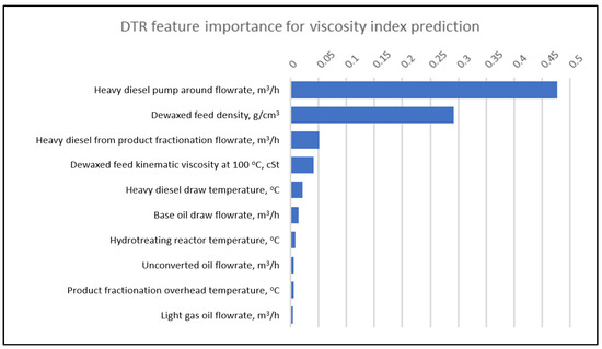
Figure 8.
Top 10 DTR features importance for viscosity index prediction.
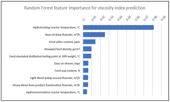
Figure 9.
Top 10 RFR feature importance for viscosity index prediction.
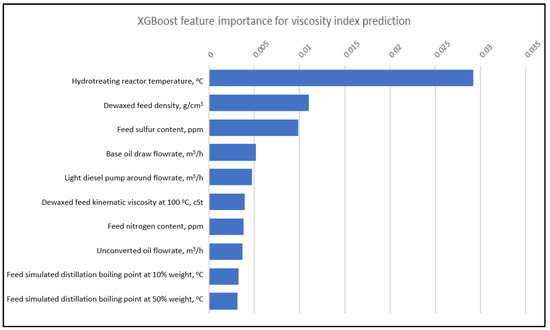
Figure 10.
Top 10 XGBoost feature importance for viscosity index prediction.
4.3. Plant Testing and Model Deployment
To assess the predictive model performance with the real time data, the models are then deployed in a platform application that is connected directly to the plant information system. A testing period is performed from 29 June 2020 until 13 January 2021. The production ran from one product grade continuously for several days and then changed to another grade continuously as per scheduled by the production planner.
Figure 11 and Figure 12 show the performance of the machine learning models in predicting the base oil kinematic viscosity at 100 °C and viscosity index, respectively. In general, XGBoost and RFR models results in lower prediction errors in comparison to DTR and SVR. Table 12 and Table 13 show the RMSE, MAE, MLSE, MAPE, R2 and Adjusted R2 values calculated from the predicted against actual for each machine learning model for both the kinematic viscosity and viscosity index output variables, respectively.
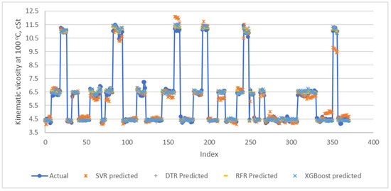
Figure 11.
Performance of each machine learning on predicting kinematic viscosity at 100 °C during model deployment.
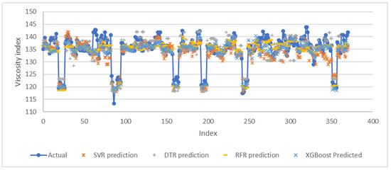
Figure 12.
Performance of each machine learning on predicting viscosity index during model deployment.
Table 12.
Performance of the machine learning models SVR, DTR, RFR and XGBoost in predicting kinematic viscosity of the base oil during the plant testing.
Table 13.
Performance of the machine learning models SVR, DTR, RFR and XGBoost in predicting viscosity index of the base oil during the plant testing.
During this plant deployment study, the SVR model provides the third best performance in predicting the viscosity index and fourth best performance for predicting the kinematic viscosity compared to the others. Comparing to RFR and XGBoost models, however, the SVR model suffers more when dealing with noises. It is observed that towards the end of the plant testing period, the prediction of the viscosity index deviated further and further from the actual value. This indicates that the SVR model requires frequent re-trainings to maintain its accuracy. Interestingly, SVR model shows a matching trend at the beginning of the index better than that of the DTR model where the prediction is more conservative in their approach by averaging the training data in its piece-wise functions. On the other hand, the XGBoost and RFR models exhibited both trending and conservative predictions which lead to better prediction accuracy.
The DTR model ranked third in predicting the base oil kinematic viscosity and fourth in predicting viscosity index. Although the DTR is a simple and very fast algorithm, it has the tendency to overfit, resulting in high bias and variance errors. The reasons that led to the overfitting could be due to the presence of noise and lack of representative instances. The bias error happens when too many restrictions are placed on the targeted functions, while the variance error is introduced by the changes of the training set. When the decision tree has high amount of variance, there is a potential to cause significant changes in the final results [32]. The base oil process dataset itself has a lot of noises which come from the interchanges of modes between 4 cSt, 6 cSt and 10 cSt, and the low frequency of feed properties lab data. Therefore, by doing a single decision tree at a time in finding the best DTR model is not as effective as the RFR and XGBoost algorithms.
Random Forest (RFR) and XGBoost models performed very well in this study. RFR model performed the best in predicting base oil kinematic viscosity at 100 °C, and XGBoost is the best at predicting the base oil viscosity index. The averaged prediction of the RFR model is expected to be closer to the true value as compared to a single decision tree. Furthermore, the RFR algorithm reduced the variance in decision trees by sampling differently during training, through the use of specified random feature subsets while also combining with shallow trees. These advantages however also comes with a cost, as the higher the number of trees that are generated in the random forest, the slower the process becomes [33]. The XGBoost algorithm, on the other hand, does not use the assumption of a fixed architecture, and instead finds the function which best approximates the data [34]. The gradient boosting algorithm finds the best parameters as well as the best function. Rather than looking for possible functions and their parameters to find the best one, which will take a very long time, it takes a lot of simple functions and adds them together. In short, the algorithm trains an ensemble of simple models. The algorithm corrects the mistakes from the first model, and the second model is trained on the gradient of error with respect to the first model’s loss predictions. Through utilization of many simple models to compensate for each other’s weaknesses, the data behavior can be learned more effectively. The DTR is a simple decision-making graph, while the RFR model is built on a large number of trees and combined using averages at the end of the process. XGBoost, on the other hand, combines the decision trees at the beginning of the process rather than the end. Gradient boosting has larger complexity in its modelling steps due to the hyperparameters tuning required, compared to RFR [33].
4.4. Product Recovery Using Prediction Model
The advantage of having a predictive model is the ability to predict the product properties in the near future, i.e., after the material has gone through the processing units (residence time). This is very useful especially during the transition between the production mode.
In this base oil production process, the most significant change in the product quality is during the transition between 10 cSt product and 4 cSt product. During this transition period, the product is diverted into a slopping tank. Previously, the decision to end the transition period is made based on the laboratory analysis results which took several hours, normally the lab result available at the 10th hours. The next challenge is to determine the right operating conditions to ensure the product will meet the specification at the end of the transition period. To solve this, the predictive model is very useful because with the given feed properties, combinations of operating condition can be entered to predict the product properties after the residence time. For this plant implementation, the XGBoost model has been utilized due to its optimal performance as shown in the earlier sections.
Therefore, performance test runs are conducted at the base oil processing plant with the aim of faster product recovery during this transition period. The 10 cSt production mode runs at lower flowrate than 4 cSt mode. Figure 13 shows the suggested feed flow rate by the model and the actual feed flowrate during the performance test run. Figure 14 and Figure 15 show hydrotreatment and hydroisomerization model suggested temperatures vs actual temperatures, respectively.
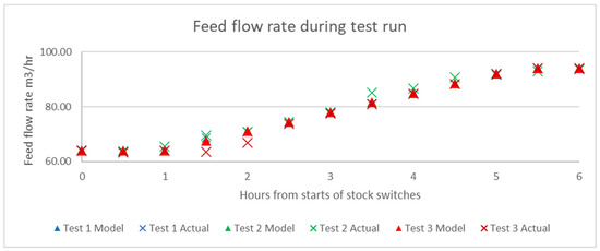
Figure 13.
Model suggested feed flowrate and actual feed flowrate during the performance test run.
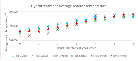
Figure 14.
Model suggested and actual hydrotreatment average reactor temperature during the performance test run.
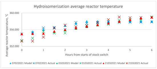
Figure 15.
Model suggested and actual hydroisomerization reactor temperature during the performance test run.
The estimated time where slopping can be ended is at the 6th hours after the transition period starts. However, samplings of the base oil product are only performed at the 4th, 5th and 6th hours because significant changes in the product properties normally happened in between the 4th to 6th hours and plant manpower optimization. The target kinematic viscosity is within the range of cSt and the viscosity index is . Figure 16 and Figure 17 shows that the product met the specification at time 6th hours, and this is achieved through the correct estimation of the appropriate operating conditions as predicted by the XGBoost model during the transition period. The transition period now has been reduced from 10 h to 6 h, a 40% improvement is observed.
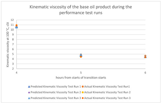
Figure 16.
Predicted and actual base oil product kinematic viscosity during the performance test run.
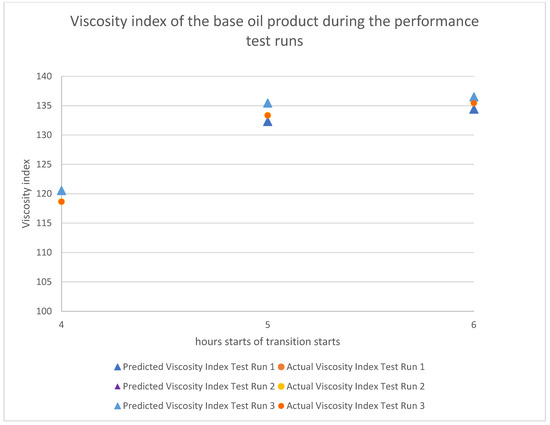
Figure 17.
Predicted and actual base oil product viscosity index during the performance test run.
5. Limitations and Assumptions
Several limitations are encountered in this study, which are amended through certain assumptions. Firstly, data from the lab are normally less frequent compared to data from equipment and transmitters. Therefore, it is assumed that the lab data, especially the feed properties, are constant until a new sample is taken. Secondly, in actual industry practice the amount of sampling and lab analysis done is normally reduced for time and cost optimization, therefore it is assumed that the data that had been used were sufficient enough to develop the model. Throughout the model development and implementation, the project team has been continuously communicating with the refinery team to obtain the best possible results. Finally, in actual operation some of the transmitters will have intermittent failures, causing historical data loss. In such cases, the operating condition values are calculated by linear interpolation.
6. Conclusions
The quality of feedstock used in base oil processing varies significantly depending on the source of the crude oil as well due to the fact that the refinery is fed with various blends of crude oil to meet the demand for the refining products. Due to cost optimization, only selected lab characterizations are performed, and the base oil processing plant is operated reactively based on the feedback of the lab analysis of the base oil product. This leads to loss in production for several hours because of the residence time as well as time required to perform the lab analysis. In this paper, a proactive method with the aim to minimize the production loss by utilizing machine learning algorithms has been carried out. Four machine learning algorithms, which are the Support Vector Regression (SVR), Decision Tree Regression (DTR), Random Forest Regression (RFR) and Extreme Gradient Boosting (XGBoost), have been studied and developed using plant historical data to predict the base oil product kinematic viscosity and viscosity index based on the feedstock qualities and the process operating conditions. The XGBoost model has shown the most optimal and consistent performance during validation and a 6.5 month plant testing periods. The benefit of the machine learning model is that it can be used to predict the product properties with the given feedstock properties and operating condition earlier than the residence time of the material moving through the operating units. The prediction model has been shown to be capable of providing the right operating conditions especially during the transitions between the production modes that allows earlier product realization compared to the reactive method. Subsequent deployment at our plant facility and product recovery analysis have shown that the prediction model has facilitated in reducing the production recovery period during product transition by 40%.
Author Contributions
Conceptualization, M.A.M.F. and A.A.R.; methodology, M.A.M.F.; software, M.A.M.F.; validation, A.A.R., M.S.R. and J.B.; formal analysis, M.A.M.F.; investigation, A.A.R.; resources, M.A.M.F.; data curation, M.A.M.F.; writing—original draft preparation, M.A.M.F.; writing—review and editing, M.A.M.F. and H.Z.; visualization, M.A.M.F.; supervision, H.Z.; project administration, J.B.; funding acquisition, J.B. All authors have read and agreed to the published version of the manuscript.
Funding
This research was funded by PETRONAS, grant number MRA grant number 015MD0-051.
Institutional Review Board Statement
Not applicable.
Informed Consent Statement
Not applicable.
Data Availability Statement
Proprietary.
Acknowledgments
The authors like to thank Universiti Teknologi PETRONAS and MRA grant number 015MD0-051 for the technical support and funding provided.
Conflicts of Interest
The authors declare no conflict of interest.
References
- Abbasi, M.; Farokhnia, A.; Bahreinimotlagh, M.; Roozbahani, R. A hybrid of Random Forest and Deep Auto-Encoder with support vector regression methods for accuracy improvement and uncertainty reduction of long-term streamflow prediction. J. Hydrol. 2020, 597, 125717. [Google Scholar] [CrossRef]
- Altgelt, K.H.; Boduszynski, M.M. Composition and Analysis of Heavy Petroleum Fractions; CRC Press: Boca Raton, FL, USA, 2016. [Google Scholar] [CrossRef]
- ASTM. Standard Practice for Calculating Viscosity Index from Kinematic Viscosity at 40 °C and 100 °C; ASTM International: West Conshohocken, PA, USA, 2010; pp. 1–6. [Google Scholar]
- ASTM. Standard Test Method for Kinematic Viscosity of Transparent and Opaque Liquids (the Calculation of Dynamic Viscosity); ASTM International: West Conshohocken, PA, USA, 2008; pp. 126–128. [Google Scholar] [CrossRef]
- Aubert, C.; Durand, R.; Geneste, P.; Moreau, C. Hydroprocessing of Dibenzothiophene, Phenothiazine, Phenozanthlin, Thianthrene, and Thioxanthene on a Sulfided NiO-MoO3/y-Al2O3. J. Catal. 1986, 97, 169–176. [Google Scholar] [CrossRef]
- Awad, M.; Khanna, R. Efficient Learning Machines; Apress Open: Berkeley, CA, USA, 2015. [Google Scholar]
- Breiman, L. Random Forests. Mach. Learn. 2001, 45, 5–32. [Google Scholar] [CrossRef] [Green Version]
- Chen, T.; Guestrin, C. XGBoost: A Scalable Tree Boosting System. In Proceedings of the 22nd ACM SIGKDD Conference on Knowledge Discovery and Data Mining, San Francisco, CA, USA, 16–17 August 2016; ACM: New York, NY, USA, 2016; pp. 785–794. [Google Scholar]
- Xgboost. Pip. 2021. Available online: https://pypi.org/project/xgboost/ (accessed on 13 January 2021).
- Chollet, F. Keras. 2015. Available online: https://keras.io (accessed on 13 May 2020).
- Cousineau, D.; Chartier, S. Outliers detection and treatment: A review. Int. J. Psychol. Res. 2010, 3, 59–68. [Google Scholar] [CrossRef]
- Drucker, H.; Surges, C.J.C.; Kaufman, L.; Smola, A.; Vapnik, V. Support vector regression machines. Adv. Neural Inf. Process. Syst. 1997, 1, 155–161. [Google Scholar]
- Fiedman, J. Greedy Function Approximation: A Gradient Boosting Machine. Ann. Stat. 2001, 1189–1232. [Google Scholar]
- Gabriel, T. Gradient Boosting and XGBoost. 1. 2018. Available online: https://medium.com/@gabrieltseng/gradient-boosting-and-xgboost-c306c1bcfaf5 (accessed on 20 May 2021).
- Glen, S. Decision Tree vs. Random Forest vs. Gradient Boosting Machines: Explained Simply. 2019. Available online: https://www.datasciencecentral.com/profiles/blogs/decision-tree-vs-random-forest-vs-boosted-trees-explained (accessed on 20 July 2020).
- Gumus, M.; Kiran, M.S. Crude oil price forecasting using XGBoost. In Proceedings of the 2017 International Conference on Computer Science and Engineering (UBMK), Antalya, Turkey, 5–8 October 2017; pp. 1100–1103. [Google Scholar] [CrossRef]
- Jiyuan, Z.; Qihong, F.; Xianmin, Z.; Chenlong, S.; Shuhua, W.; Kuankuan, W. A supervised Learning Approach for Accurate Modeling of CO2-Brine Interfacial Tension with Applicaiton in identifying the Optimum Sequestration Depth in Salin Aquifers. Energy Fuel 2020, 34, 7353–7362. [Google Scholar]
- Louppe, G. Understanding Random Forests: From Theory to Practice. Ph.D. Thesis, University of Liège, Liège, Belgium, 2015. [Google Scholar]
- Lynch, T.R. Process Chemistry of Lubricant Base Stocks, 1st ed.; CRC Press: Boca Raton, FL, USA, 2007. [Google Scholar]
- Machado, G.; Mendoza, M.R.; Corbellini, L.G. What variables are important in predicting bovine viral diarrhea virus? A random forest approach. Vet. Res. 2015, 46, 1–15. [Google Scholar] [CrossRef] [PubMed] [Green Version]
- Markovic, S.; Bryan, J.L.; Ishimtsev, V.; Turakhanov, A.; Rezaee, R.; Cheremisin, A.; Kantzas, A.; Koroteev, D.; Mehta, S.A. Improved Oil Viscosity Characterization by Low-Field NMR Using Feature Engineering and Supervised Learning Algorithms. Energy Fuels 2020, 34, 13799–13813. [Google Scholar] [CrossRef]
- Meng, M.; Zhong, R.; Wei, Z. Prediction of methane adsorption in shale: Classical models and machine learning based models. Fuel 2020, 278, 118358. [Google Scholar] [CrossRef]
- Mokhatab, S.; William, A.P. Chapter 15—Process Modeling in the Natural Gas Processing Industry. In Handbook of Natural Gas Transmission and Processing, 2nd ed.; Mokhatab, W.A.P.S., Ed.; Gulf Professional Publishing: Waltham, MA, USA, 2012; pp. 511–541. [Google Scholar]
- Moreau, C.; Aubert, C.; Durand, R.; Zmimita, N.; Geneste, P. Structure-Activity Relationships in Hydroprocessing of Aromatic and Heteroatomic Model Compounds Over Sulphided NiO-MoO3 y-Al2O3 and NiO-WO3 y-Al2O3 Catalysis: Chemical Evidence for the Existence of Two Types of Catalytic Sites. Catal. Today 1988, 4, 117–131. [Google Scholar] [CrossRef]
- De Myttenaere, A.; Golden, B.; Le Grand, B.; Rossi, F. Mean Absolute Percentage Error for Regression Models. Neurocomputing 2016, 192, 38–48. [Google Scholar] [CrossRef] [Green Version]
- Nag, N.K.; Sapre, A.V.; Broderick, D.H.; Gates, B.C. Hydrodesulfurization of Polycyclic Aromatics Catalyzed by Sulfided CoO-MoO3 y-Al2O3: The Relative Reactivities. J. Catal. 1979, 57, 509–512. [Google Scholar] [CrossRef]
- Pedregosa, F.; Varoquaux, G.; Gramfort, A.; Michel, V.; Thirion, B.; Grisel, O. Scikit-Learn: Machine Learning in Python. 2011, pp. 2825–2830. Available online: https://scikit-learn.org/ (accessed on 15 February 2020).
- Platt, J.C. Probabilistic outputs for support vector machines and comparisons to regularized likelihood methods. Adv. Large Margin Classif. 1999, 10, 61–74. [Google Scholar]
- Rudin, C. Support Vector Machines MIT 15.097 Course Notes. 2012, pp. 1–14. Available online: http://ocw.mit.edu/courses/sloan-school-of-management/15-097-prediction-machine-learning-and-statistics-spring-2012/lecture-notes/MIT15_097S12_lec12.pdf (accessed on 3 April 2021).
- Üstün, B.; Melssen, W.J.; Buydens, L.M.C. Visualisation and interpretation of Support Vector Regression models. Anal. Chim. Acta 2007, 595, 299–309. [Google Scholar] [CrossRef] [PubMed]
- Vapnik, V.N. Statistical Learning Theory; Wiley: New York, NY, USA, 1998. [Google Scholar]
- Wilkinson, L. Classification and Regression Trees. 1995. Available online: http://cda.psych.uiuc.edu/multivariate_fall_2012/systat_cart_manual.pdf (accessed on 16 January 2021).
- Zhang, J.; Feng, Q.; Wang, S.; Zhang, X. Estimation of CO2-Brine Interfacial Tension Using an Artificial Neural Network. J. Supercrit. Fluids 2016, 107, 31–37. [Google Scholar] [CrossRef]
- Zhong, R.; Johnson, R.; Chen, Z. Generating pseudo density log from drilling and logging-while-drilling data using extreme gradient boosting (XGBoost). Int. J. Coal Geol. 2020, 220, 103416. [Google Scholar] [CrossRef]
Publisher’s Note: MDPI stays neutral with regard to jurisdictional claims in published maps and institutional affiliations. |
© 2021 by the authors. Licensee MDPI, Basel, Switzerland. This article is an open access article distributed under the terms and conditions of the Creative Commons Attribution (CC BY) license (https://creativecommons.org/licenses/by/4.0/).