The Corona Phenomenon in Overhead Lines: Critical Overview of Most Common and Reliable Available Models

Abstract

Research on corona discharge, shared by physics, chemistry and electrical engineering, has not arrested yet. As a dissipative process, the development of corona increases the resistive losses of transmission lines and enhances the line capacitance locally. Introducing additional losses and propagation delay, along the line, non-linearity and non-uniformity of the line parameters; therefore, corona should not be neglected. The present work is meant to provide the reader with comprehensive information on the corona macroscopic phenomenology and development, referring to the most relevant contributions in the literature on this subject. The models proposed in the literature for the simulation of the corona development are reviewed in detail, and sensitivity curves are provided to highlight their dependence on the input parameters.

1. Introduction

Corona may be defined as a non-linear phenomenon involved in the initial phase of electrical discharges, resulting in the flow of electric energy from a conductor to the ionized medium [1]. It consists of self-contained localised discharges and of the proximity of electrode surfaces characterized by local high intensity electric fields, stressing the insulating strength of the surrounding dielectric medium [2]. The phenomenon was studied rigorously for the first time by Faraday in 1838 [3].

Some of the very first references to this phenomenon date back to 1838, when Michael Faraday noticed a “quiet phosphorescent continuous glow”, and stated that “that form of disruptive discharge which appears as a glow […] seems to depend on a quick and almost continuous charging of the air close to, and in contact with, the conductor” [3].

Early relevant and extensive studies on corona were performed by Peek in the first decades of the 20th century [4,5]; when applying a threshold voltage to a conductor, a “hissing noise” and a pale luminosity were observed in the proximity of its surface [6]. Indeed, the high frequency spectra typical of discharge processes result in the emission of audible noise and radio interference in the MHz range, research being oriented toward prediction and mitigation of these dissipative side effects [7].

Interaction between charged particles under the accelerating effect of an external electric field, turning into an avalanche phenomenon and, finally, into a process of local discharge by breakdown of the insulating medium, raised the interest of industries. The mechanism of recombination of ionized oxygen atoms, resulting from the discharge process, and oxygen molecules in the air is exploited for the production of ozone (O${}_3$) on a utility-scale through ozone generators operated by corona technology [8], which need to trigger efficient discharges in a controlled environment in order to optimize ozone production.

Therefore, since Peek’s early works on this topic, a relevant contribution, supported by experimental data, was represented by the book of Gary and Moreau [9], addressing also the computation of the localised losses caused by the corona discharge. Researchers further investigated the dependence of the inception electric field on environmental and atmospheric conditions [10], electric field distribution [11], polarity and steepness of the applied voltage waveform [12]. On the other side, some authors proposed techniques to account for the typical hysteretic relation between charge and voltage. The proposed models, which are reviewed in this work, are aimed at evaluating the effects of corona on surge propagation along transmission lines, and differ in the adopted approaches and in the simplifying assumptions made, and hence, in their range of applicability and complexity of implementation. Furthermore, the reviewed models have been frequently validated through comparison of results with specific experimental data, which are not sufficient to ensure their general validity. In fact, prior tuning of the parameters required by each model is fundamental when it comes to reproducing measured data.

The present review is organized as follows: some insights on side effects related to corona, i.e., audible noise, radio interference, and luminosity, are given in Section 2. In Section 3, the main physical mechanisms underlying corona inception and development are described, and reference is made to the hysteretic relation between charge and voltage; different expressions for the computation of the inception electric field $E_{\mathrm{inc}}$ are introduced as well. In Section 3.4, we provide insight on the role played by the irregularity factor m in the computation of $E_{\mathrm{inc}}$ for stranded conductors or bundles. In Section 4, corona models available in the literature are reviewed in detail and classified in physics-based models, empirical models, and models suitable to be included in any commercial transients programs for circuit analyses. Finally, conclusive comments may be found in Section 7.

2. Main Corona Effects

When dealing with power delivery by high voltage transmission lines in air, corona discharge may be responsible for additional losses when the line design and specific operation conditions lead to corona inception. In fact, if the high voltages applied to the conductors—guaranteeing the efficiency of energy transport at large distances—result in electric fields exceeding the insulating strength of the air in the proximity of the conductors, localised discharge processes may enhance per-unit length (p.u.l.) losses [13]. This effect, undesired in normal operation conditions, may turn beneficial when unpredictable overvoltages (e.g., traveling lightning surges) propagate along the line, threatening electrical devices essential for the service continuity; along with the attenuation of traveling waves peak value, a reduction in the surges’ propagation velocity may be observed, associated with the increased capacitive behavior of the line under corona conditions [14]. Section 4 is devoted to the detailed discussion of these latter aspects, while other non-negligible side effects associated with corona, i.e., luminosity, audible noise, and radio interference, are addressed in the following sections.

2.1. Luminosity

Laboratory measurements have shown characteristic patterns of the optical spectra in the proximity of test conductors under corona [15]; indeed, when the wavelength of corona emitted fields ranges between 380 nm and 780 nm, i.e., in the visible spectrum for the human eye, corona may be further detected by a visible violet luminosity [2]. Interestingly, corona glow, with a spectrum up to UV, in addition to representing an effective detection tool, also caught the attention of researchers on the impact of this phenomenon on wildlife [16].

2.2. Audible Noise

An additional side effect of corona discharge is related to the emission in the audible spectrum (approximately in the range 20 Hz–20 kHz). The total emitted noise, similar to a buzzing sound, may be considered the superposition of broadband and single-tone components; the former is associated to discharges localised in the proximity of the conductor surface, causing rapid variations in air pressure, due to intense local heating [7]; single-tone components, observed in the case of intense corona along a.c. lines at frequencies of twice the operation value, are associated with space charge movement under the effect of the alternating electric field [17].

2.3. Radio Interference

At higher frequencies, in the range between 0.01 MHz and 30 MHz, radio interference (RI) is a well-known disturbance phenomenon, which may be caused by corona development in proximity of HV d.c. and a.c. lines, affecting the quality of AM radio broadcasting [18]. The International Special Committee on Radio Interference (CISPR), involved in EMC issues and standardization, addresses this topic in detail in [19], with reference to RI due to overhead power lines. To assess the impact of corona on signal transmission at radio frequencies, three aspects are considered: frequency spectrum, lateral profile (i.e., attenuation of the field at ground level in the direction perpendicular to the source), and statistical distribution, to be evaluated following proper measurement procedures [18,20]. Indeed, different weather conditions, features of the conductors surface (e.g., dirt, irregularities, etc.) strongly affect RI levels, up to 20–30 dB [21], and may be taken into account through long-term surveys and statistical analysis. Several empirical and analytical approaches have been proposed in the literature to predict the impact of corona audible noise and RI on the surrounding environment [22] under variable atmospheric conditions, and guide overhead HV lines and substations design to limit emissions.

3. Corona Inception and Development

Corona is a self-sustained discharge process, developing in regions with high-intensity electric fields, which includes ionization of the surrounding dielectric medium, drift and diffusion of charged species, i.e., electrons, or charged atoms or molecules [23]. Microscopic or macroscopic approaches may be adopted to study and simulate this phenomenon.

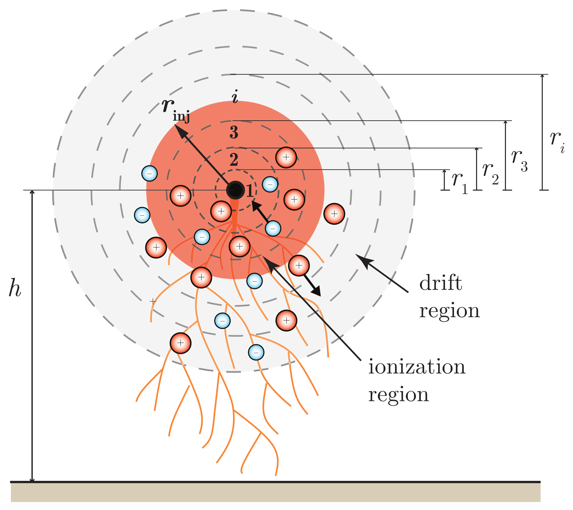
3.1. Microscopic Level

In order for the corona inception to happen, a ionization process needs to be started by the production of ions and electrons at an exponential rate, also denoted as an avalanche mechanism, which was first addressed by Townsend [24]. With reference to a cylindrical electrode in the air at atmospheric pressure, the main process involved in avalanches development is ionization of neutral molecules by the collision with primary electrons; indeed, these electrons may be available in low concentration in the atmosphere and accelerated by the external electric field, or may be detached from existing negative ions and accelerated until collision. A statistical time lag ${\tau }_{\mathrm{st}}$, in the range of $\mathsf{\mu }$s, is necessary for the formation of enough primary electrons to start the avalanche process. Experimental evidence showed ${\tau }_{\mathrm{st}}$ to depend on the availability of free electrons, and on the rate of rise of the applied voltage; lower mean values of ${\tau }_{\mathrm{st}}$ are associated with steeper voltage fronts [2]. Ionization by impact is generally modeled by Townsend’s coefficient $\alpha$, which accounts for the average number of ionizing collisions expected for a single electron along a 1 m path and depends on the air pressure and electric field distribution [25].

When all the primary electrons are involved in collisions, secondary electrons are necessary to act as “seeds” for the following avalanches. They may be produced by several mechanisms, e.g., photoionization for positive corona, which consists in the production of positive ions and electrons resulting from photon–molecule interactions [26], and secondary emission for negative corona, which corresponds to electrons emission by positive ions approaching the electrode surface and being successively neutralized [27].

Outside the ionization region, the only processes of interest are charge movement through drift (depending on the electric field and ion/electron mobility) and diffusion of charged species (linked to the gradient of the space charge density and ion/electron diffusivity), and subtraction of space charge through recombination and attachment. Furthermore, corona experimental evidences have shown different discharge modes with respect to a DC or AC applied voltage source.

DC, AC, Impulse Corona

Depending on the nature of the voltage source applied to the electrode under test, different corona modes develop; the work by Giao and Jordan [28] displays a detailed analysis on this topic, whose fundamental aspects are reported here:

• Negative DC corona: when a negative polarity voltage close to the inception value is applied, negative corona starts in the form of current pulses, known as “Trichel pulses”; the pulses’ frequency increases with the increasing value of the applied voltage. The intermittent nature of these localised discharges is related to the space charge, which contribute to weaken the electric field in the electrode proximity (holding back the pulses) and to subsequent space charge removal. Further increase in the voltage leads to a pulseless glow, which may turn into negative streamers of growing length if the voltage reaches values close to the insulation breakdown [13].
• Positive DC corona: from experimental data [29], the inception voltage for positive DC corona is slightly lower, compared to negative DC corona. According to [28], this is reasonably due to the electrons being accelerated in the direction of the increasing electric field, i.e., towards the anode, facilitating ionization processes. Mixed opinions may be found in the literature on this subject; for instance, in [13], corona discharge due to negative polarity applied voltages is stated to occur at lower field values, with respect to positive polarity (the difference being enhanced when sharp-shaped electrodes are considered). This is in accordance with experimental values found in [30], and with values for the critical corona onset gradient in [31]. However, it is shared opinion that experimental activities aimed at assessing the corona onset field are strongly dependent on atmospherical conditions, humidity, configuration and available free charges in the vicinity of the conductor under test. Fundamental steps in the study of positive DC corona are found in [32]. It first develops in the form of burst pulses; depending on the electrode radius, gap length and magnitude of the applied voltage, some onset streamers may be produced as well, reaching larger radial distances from the electrode and being choked off by negative ions in the gap. Increasing voltage and higher densities of negative space charge suppress the onset streamers in favor of a diffused glow in the proximity of the anode (Hermstein’s glow); streamers finally causing the insulation breakdown are observed at higher voltages, developing from the glow region [28].
• AC corona: when a sinusoidal voltage source triggers corona, combined modes typical of positive and negative DC corona may be observed. In particular, a critical distance can be introduced, depending on the voltage peak value and frequency, accounting for the path covered by the charge particles during the quarters of periods from the voltage peaks to zero crossings; if the critical distance is such that no residual space charge is left by the end of the half period (i.e., suitable time has passed for the ions to migrate toward the electrode of opposite polarity and being neutralized), corona modes in the positive and negative half cycles are expected to be equal to the DC modes with corresponding polarity. Otherwise, the residual space charge will influence the development of the corona modes during the subsequent half-cycle with opposite polarity [28].
• Impulse corona: with fast front voltages, corona mainly develops in the streamer mode, being the role played by the space charge limited by its slower dynamics [33].

3.2. Macroscopic Level

Ionization and interactions among charges at microscopic level provoke a non-linear and hysteretic relation between the total charge and the voltage at the electrode surface at macroscopic level, as sketched in Figure 1. When a monotonically increasing voltage is applied to a reference conductor, a proportionality factor, i.e., the conductor capacitance, governs the q-v relation until corona develops, in correspondence to the inception voltage $V_{\mathrm{inc}}$; a further voltage increase results in the space charge growing at a rate faster than linear, albeit delayed of time ${\tau }_{\mathrm{sp}}$ in the range between 25 $\mathsf{\mu }$s and 100 $\mathsf{\mu }$s in the hemisphere-plane gap configuration, depending on the gap length, and on the voltage rate of the rise and peak value [2,34] necessary for its formation [26]. Due to this delay time ${\tau }_{\mathrm{sp}}$, the peak value of the charge may be observed when the time derivative of the applied voltage has already reversed in sign; at later times, for decreasing values of voltage, the linearity of the q-v relation is restored. The last branch of the loop (D and E in Figure 1) shows a larger slope with respect to the one of branches C and D. At point E, the dynamic and the magnitude of the electric field produced by the applied source are no longer predominant, compared to the electric field produced by the space charge, which contributes to the mechanism of space charge subtraction, resulting in a value of the derivative $\mathrm{d}q/\mathrm{d}v$ larger than $C_{\mathrm{geo}}$ [35].

Numerous experimental activities [12,36], supported by theoretical considerations [2], have put in evidence that the electric field inception value $E_{\mathrm{inc}}$ depends on the steepness of the applied voltage. As a result, different formulae for the computation of $E_{\mathrm{inc}}$ have been proposed in the literature.

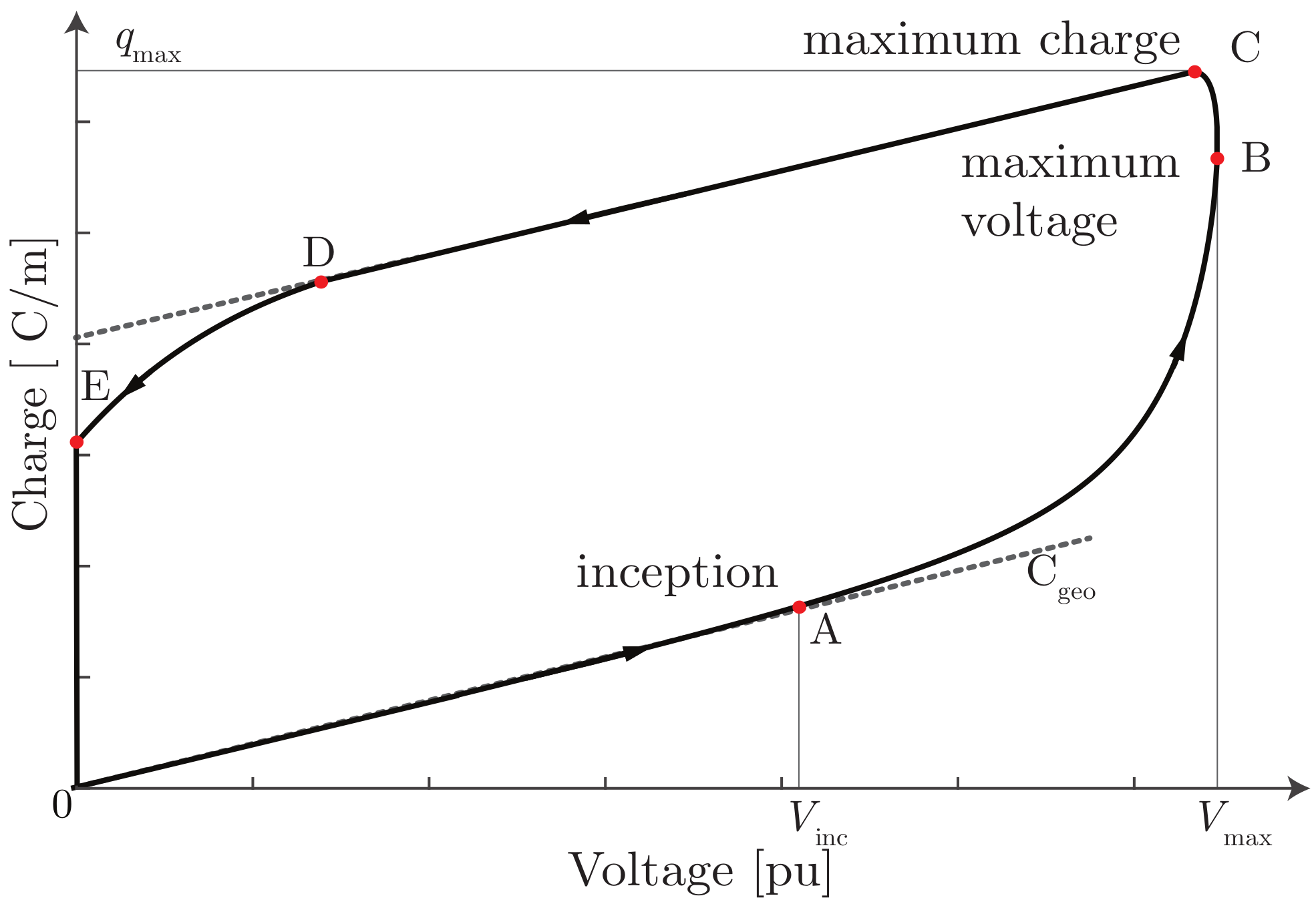
3.3. Inception Criterion

In this section, the approaches from Peek [5], Olsen and Yamazaki [11], and Mikropoulos et Zagkanas [37] are reviewed, their applicability is clarified, and the main ideas and considerations underlying the formulation are discussed. The majority of the approaches do not consider the influence of the steepness of the applied voltage on the value of the inception field, their validity being limited to DC or power frequency applications. Criteria accounting for this aspect, as well as for non-coaxial arrangements for the direct application to transmission lines (TLs) studies, are found to be lacking in the literature.

Since these criteria refer to solid conductors, a correcting factor, i.e., the irregularity factor, is often exploited to compute the inception voltage associated with stranded conductors and bundles. Its role is also discussed in this section.

3.3.1. Inception Field by Peek

Early experimental research activities by Peek [4,5,6] led to the well-known expression for the critical inception field $E_{\mathrm{inc}}$ of the insulating air, i.e., the value of the electric field at which visual effects of corona, such as luminosity of the air surrounding the conductor, may be first observed:

$$E_{\mathrm{inc}}=30·m\delta f_{\mathrm{p}}\left(1+\frac{K_{\mathrm{p}}}{\sqrt{\delta r_0}}\right)=E_0\left(1+\frac{K_{\mathrm{p}}}{\sqrt{\delta r_0}}\right),$$

(1)

where $K_{\mathrm{P}}=0.3$ in the original formulation by Peek. As expected, the inception field in (1), expressed in kV/cm, only depends on the conductor radius $r_0$, and not on any other geometrical feature of the configuration under test (which, on the contrary, affects the onset voltage); $\delta$ is the air density factor, and $f_{\mathrm{p}}$ is the polarity factor, which takes into account the effect of voltage polarity on $E_{\mathrm{inc}}$ since experimental evidence has shown that the inception electric field associated with positive corona may hold different values with respect to those related to negative corona (with reference to the coaxial configuration, [38]); m is a constant to take into account the irregularity of the conductor surface, distinguishing between perfectly smooth conductors and rough surfaces due to weather conditions and aging under operation. From the manipulation of (1), assuming $\delta =1$ and axial-symmetric configuration, Peek’s criterion may be alternatively interpreted as the value of the electric field at the conductor surface allowing to reach a field equal to $E_0$ at distance $\tilde{r}=r_0+0.301\sqrt{r_0}$ from the conductor axis, $E_0$ being independent from the configuration under analysis. Indeed, according to (1), the inception field holds higher values for conductors, presenting a smaller radius $r_0$, as the proposed formula, although expressed in terms of $r_0$, relies on a requirement for the electric field at $\tilde{r}$.

In the literature, many empirical expressions similar to (1) may be found, computing $E_{\mathrm{inc}}$ through the following general relation:

$$E_{\mathrm{inc}}=A\delta \left(1+\frac{B}{{\left(\delta r_0\right)}^C}\right),$$

(2)

where coefficients A, B, and C (ranging between 23–35, 0.15–1, and 0.3–0.5, respectively) hold different values for the different expressions proposed in the literature, which are classified in [39] for d.c. corona.

3.3.2. Inception Field by Olsen and Yamazaki

When dealing with the evaluation of corona inception field at power frequencies, the onset criterion by Olsen and Yamazaki [11] takes into account the predominant interactions among free charges in proximity of the conductor; in particular, differently from the approaches in Section 3.3.1, the proposed corona onset criterion is associated not only with the maximum electric field at $r_0$, but also with the electric field trend in the area surrounding the conductor surface, still not accounting for any steepness effect by the applied voltage. Two main phenomena are considered: charge formation through impact ionization, and space charge reduction through attachment. The former phenomenon is associated with Townsend’s first ionization coefficient $\alpha$, the latter with the attachment coefficient $\eta$. The inception criterion, derived from corona onset experimental data, is expressed by the following analytical condition:

$$\frac{K\left(r_0+{\delta }_0\right)}{K\left(r_0\right)}=\exp \left({\int }_{r_0}^{r_0+{\delta }_0}\left(\alpha -\eta \right)ds\right)\ge 3500.$$

(3)

In (3), $K\left(r\right)$ represents the number of free electrons at distance r from the conductor axis. Coefficients $\alpha =\alpha \left(p,E\right)$ and $\eta =\eta \left(p,E\right)$ have to be intended as functions of the air pressure p and of the instantaneous electric field $E\left(r\right)$, assumed radial; ${\delta }_0$ denotes the thickness of the corona layer, to be intended as the distance from the conductor surface at which free charges produced by impact ionization and those canceled by attachment are equal, i.e., the distance where the following condition is verified:

$$\alpha \left(p,E\left(r_0+{\delta }_0\right)\right)=\eta \left(p,E\left(r_0+{\delta }_0\right)\right).$$

(4)

Expressions for $\alpha$ and $\eta$ can be found in [40], and read as follows:

$$\alpha \left(p,E\right)=\left\{\begin{array}{cc}4.7786p{\mathrm{e}}^{-0.221\frac{p}{E}},\hfill & \mathrm{for}0.025\le \frac{E}{p}\le 0.060\hfill \\ 9.682p{\mathrm{e}}^{-0.2642\frac{p}{E}},\hfill & \mathrm{for}0.060<\frac{E}{p}<0.24\hfill \end{array}\right.$$

(5)

$$\eta \left(p,E\right)=0.01298p-0.541E+8.7\frac{E^2}{p},$$

(6)

where E is expressed in kV/cm and p in mmHg. Both the coefficients $\alpha$ and $\eta$ are computed considering that the space charge influence on the electric field is negligible before inception occurs. This assumption made, starting from the configuration under study, i.e., coaxial arrangement, or conductor above a perfect electric conductor (PEC) surface, and the conductor features (i.e., single conductor of radius $r_0$, or stranded conductor), the electric field $E\left(r\right)$ to be plugged into (5) and (6) may be found from the known applied voltage. Hence, relations (5) and (6), along with the trend of the electric field surrounding the conductor, have to be taken into account simultaneously to compute the inception value of $E_{\mathrm{inc}}$ through the solution of Equation (3).

3.3.3. Inception Field by Mikropoulos and Zagkanas

A modification to the general formula (2) for the inception electric field (in kV/cm) is proposed by Mikropoulos and Zagkanas in a coaxial arrangement [37]:

$$E_{\mathrm{inc}}=K_s·31.53\left(1+\frac{0.305}{\sqrt{r_0}}\right)$$

(7)

where

$$K_s=0.42·\mathrm{sign}\left({\left.\frac{\mathrm{d}v}{\mathrm{d}t}\right|}_{10/90}\right){\left|{\left.\frac{\mathrm{d}v}{\mathrm{d}t}\right|}_{10/90}\right|}^{0.345}$$

(8)

where the voltage time derivative at the right-hand side of (8) is the steepness of the applied voltage in kV/$\mathsf{\mu }$s, assuming its waveform to increase linearly between 10% and 90% of its peak value. In fact, experimental data from [37] are in good agreement with Peek’s inception field only in the case of slow-front voltage sources (up to 10 kV/$\mathsf{\mu }$s); when different impulse voltages are applied to a reference conductor, electric field onset values show a dependence on the impulse steepness, which is neglected in expressions based on Peek’s formula. Hence, the steepness correction factor (8) is introduced to take into account the increase in $E_{\mathrm{inc}}$ with steeper fronts of the applied voltage.

3.4. Role of the Irregularity Factor: Stranded Conductors and Bundles

In the current section, some more in-depth information will be given about the irregularity factor m, when dealing with stranded conductors and bundles.

This factor allows to evaluate the corona inception field of any conductor, starting from $V_{\mathrm{inc}}$ computed for a reference conductor with the same outer diameter and smooth cylindrical surface. Indeed, m may include also several physical or geometrical features of the conductor generating irregularity, i.e., grease, dirtiness or dust, and scratches. Several tests were conducted by Baker et al. [41], showing the influence of surface irregularities on corona development in heavy rain conditions, or for wet surface/foggy weather; differences were observed between new (as from manufacturer) and aged conductors, the former showing more pronounced corona activity with heavy rain [41]. This is attributed to the greased surface, which causes water to lay in droplets, enhancing locally the electric field. Aged conductors, instead, show hydrophilic behavior, letting the water flow toward their underside. Hence, factor m might take a different value, depending on the conductor aging process. Instead, the effect of the aging process of conductors operating in polluted areas, i.e., the increased roughness of their surface, is investigated in [42].

3.4.1. Stranded Conductors

When dealing with stranded conductors, the diameter of the external strands, and their arrangement affect the value of the inception voltage; it is usually taken into account through the stranding factor, defined as the ratio between $V_{\mathrm{inc}}$ computed for the stranded conductor, and $V_{\mathrm{inc}}$ of a smooth conductor sharing the same outer diameter [43].

Experimental data on the stranding factors with stranding ratios (i.e., ratio between the diameter of any external strand and the outer diameter of the conductor) in the range $0.05÷0.25$ and different conductors diameters were collected by Stone [43]. As expected, the found values converge to 1 for the smallest stranding ratios; for the growing stranding ratio, the stranding factor is found to decay faster when dealing with larger conductors, suggesting that the inception of corona may not be related only to the maximum value of the electric field on the surface of the strands.

Hence, Yamazaki and Olsen [11] elaborated the inset criterion, reviewed in Section 3.3.2, based on the electric field distribution in the proximity of the conductor.

This criterion justifies the values assumed by the stranding factor, i.e., the reduced $V_{\mathrm{inc}}$ at which the corona inception is observed; the stranded surface results in a different electric field distribution, and in the enhancement of its maximum value with respect to the case of a smooth conductor for a given voltage.

Even though we have referred to the potential, since it is often used in numerical codes as a threshold value for the simulation of the corona inception, the electric field distribution is the primary cause of corona. Bousiou et al. [38] showed the trend of the electric field magnitude at increasing distance from the conductor outer radius $r_0$, for different stranding ratios, showing that, for $r\to r_0$, the electric field for stranded conductors tends to a value approximately equal to 1.4 times $E_{\mathrm{inc}}$ for the corresponding smooth conductor, independently from the number of external strands; however, as expected, the trend of $E\left(r\right)$ approximates that of smooth conductors as the number of external strands increases. Furthermore, at equal applied voltage, the electric field holds higher values with a decreasing number of strands, also at larger distance from the conductor axis [44]; it is reasonable that the inception depends on the distribution of the electric field and not only on its maximum value; thus, lower values of $E_{\mathrm{inc}}$ found for higher stranding ratios [38] are justified.

When accounting for the stranding, misleading interpretation may occur about the role played by the surface regularity factor m in (1). In fact, only $V_{\mathrm{inc}}$, as a function of the stranding factor, effectively decreases, due to stranding. Hence, the value of $E_{\mathrm{inc}}$, with the irregularity factor m, corresponds to the inception field of an equivalent smooth conductor sharing the same inception voltage with the original stranded one, but $not$ the same inception field at the surface.

3.4.2. Bundles

The technical solution of bundle conductors, for high-voltage transmission applications, is well-known for increasing lines loadability and reducing the occurrence of corona; this latter effect has been largely investigated in the literature, especially with the increasing spread of EHV and UHV lines.

Peek formula (1) does not apply to bundle configurations; research has been conducted to establish a suitable corona inception criterion. Waiving the approximation of uniform radial distribution of the electric field, it is necessary to refer to the maximum value $E_{max}$ attained by the electric field in the bundle proximity, which can be computed through the charge simulation method [45], or approximately for the coaxial configuration [46] and for bundles over a conductive plane [47] through the general formula as follows:

$$\begin{array}{}\mathrm{(9a)}& E_{\max }=E_{\mathrm{av}}\left[1+\left(n-1\right)\frac{r_0}{r_{\mathrm{b}}}\right]\hfill \mathrm{(9b)}& E_{\mathrm{av}}=\frac{1}{n{r}_0}{e}_{\mathrm{av}}\left(r_{\mathrm{eq}},v,d\right),\hfill \end{array}$$

where n is the number of subconductors of radii $r_0$ of the bundle; $r_{\mathrm{b}}$ is the bundle radius; v is the voltage applied to the subconductors of the bundle; d denotes the radius of the external conductive cylinder in the coaxial configuration, or the height of the bundle over the conductive plane; and $r_{\mathrm{eq}}={\left(n{r}_0{r}^{n-1}\right)}^{1/n}$ is the equivalent radius of the bundle [47].

Indeed, the exact solution of the electrostatic problem of charged cylinders over a conductive plane, also accounting for proximity effects, was solved through conformal mapping in [48].

Data presented by Maruvada et al. in [36] show a slight increase in the corona inception field for bundles with respect to single conductors; indeed, in the former case, charged ions and electrons might need an increased electric field to properly start an avalanche, due to the asymmetric radial distribution. Nevertheless, the authors of [46] observed that $V_{\mathrm{inc}}$ for bundle configuration may be estimated satisfactorily by the applied voltage, causing $E_{max}$ to be equal to the inception field of any of the subconductors, as if it was alone on the ground.

The influence of the number of subconductors and bundle radius was assessed in [46]. In particular, while increasing the number of subconductors always results in a reduced maximum electric field, and hence, in a higher inception voltage, the dependence on the bundles radius is more complex. For a fixed number of subconductors, an optimum bundle radius can be identified, which maximizes the inception voltage (associated with the configuration generating the weakest $E_{max}$).

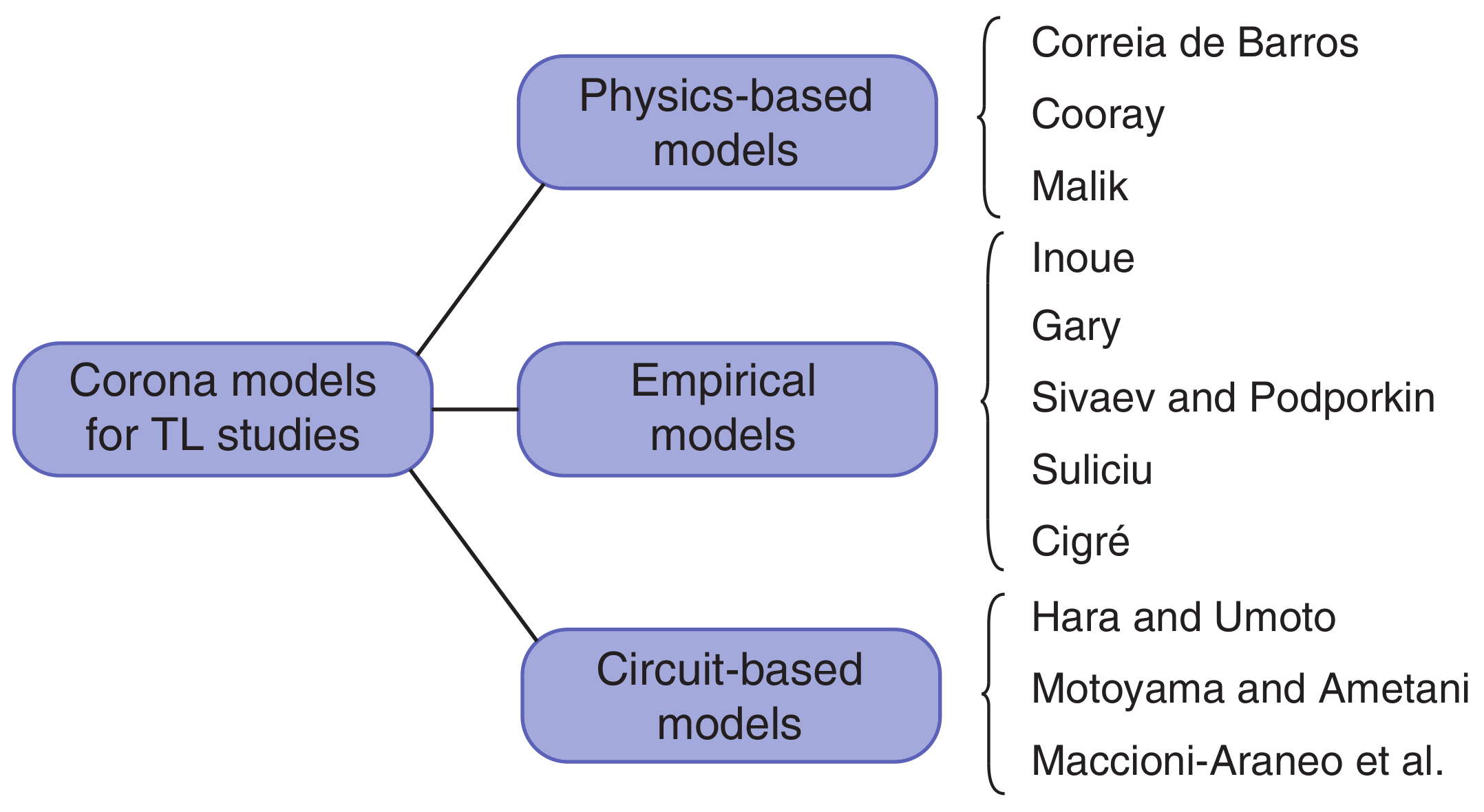
4. Models for Corona Simulation

In the literature, several models are available for the simulation of the corona phenomenon, in order to reproduce the multi-valued hysteretic relation between the charge and the voltage. The most relevant models included here were classified as in

Table 1. Main models for corona effect simulation.

	Model	Ref.	Model Features	Related
Physics-based models	Correia de Barros	[35,52,53,54]	Multi-layer space discretization, solution of drift equations	[55]
	Malik et al.	[56]	One-layer model with time dependent radius	[57,58]
	Cooray	[59]	One-layer model with time dependent radius	[60]
Empirical models	Inoue	[61]	Expression of the corona capacitance	-
	Gary et al.	[62]	Expression of the total charge	-
	Podporkin and Sivaev	[63]	Expression of the total charge	-
	Suliciu et al.	[64]	Expression of the corona over-current	[65]
	CIGRÉ	[66]	Expression of the corona dynamic capacitance	[67]
Circuit models	Hara and Umoto	[68]	Voltage-dependent shunt capacitor and resistor	[69]
	Motoyama and Ametani	[70]	Shunt capacitor and resistor, piece-wise constant functions of the voltage	-
	Maccioni, Araneo et al.	[71]	Voltage-dependent current generator and shunt resistor	-

, according to the different approaches adopted for their formulation. It should be noted that the following models are the preferred choice when the effect of corona discharge needs to be considered in TL studies with respect to multi-species discharge models. In fact, despite being more accurate and adherent to the physical reality, the latter models require larger computation times, usually by means of the finite element method (FEM) with a suitable iterative solver for the solution of non-linear charge transport equations. The diagram in Figure 2 shows, at a glance, the models here reviewed.

We refer to the first subset as “physics-based” models. These models use a simplified description of the physical mechanisms underlying the corona phenomenon, which would require a coupled electro-fluid dynamic plasma model to be fully determined [49,50]. Complexity arising is the main drawback of such detailed models, which conflict with the aim of formulating simple tools suitable for engineering purposes. Nonetheless, the main advantage of their application consists in their general applicability, through non-linear relations accounting for all the key physical aspects from a macroscopic point of view. In these models, corona losses derive directly from the area described by the q-v hysteretic curve and hence, no additional conductance is introduced.

Starting from measured q-v curves in known configurations, “empirical” models attempt to define $q^{\prime }$ or $C^{\prime }$ (p.u.l. quantities) as a function of the applied voltage in order to approximate the measured data. The most remarkable advantage is the easiness of their implementation; as a downside, they all require a careful choice of the values of a set of input parameters in order to obtain q-v curves close to those resulting from measurements.

Finally, availability of transient-programs (e.g., ATP/EMTP, PSCAD) has fostered the development of “circuit-based” corona models to be easily implemented in conjunction with widely tested models of multiconductor TLs and other equipment. Circuit-oriented models introduce shunt circuital elements to reproduce the propagation effects of corona phenomenon, i.e., attenuation and time delay. The additional lumped components may be generally expressed as the product of some p.u.l. voltage-dependent electrical parameters (i.e., $C^{\prime }$, $G^{\prime }$) and the spacing $\mathsf{\Delta }\ell$ adopted for the insertion of these equivalent additional shunt circuits. Their circuit structure reveals an advantage for the implementation in commercial transients programs, through simple construction of equivalent circuits to be plugged to the line under study. As a drawback, these models compute attenuation and delay due to corona only at chosen voltage nodes, simulating a phenomenon which is actually distributed as a lumped equivalent one.

We note that both the empirical and the circuit-based models may lead to the definition/computation of a voltage-dependent, i.e., time-varying, capacitance; strictly speaking, if the conductor capacitance is assumed to be non-constant, the associated p.u.l. capacitive current $i_{\mathrm{c}}^{\prime }$ should be computed as follows:

$$i_{\mathrm{c}}^{\prime }\left(t\right)=\frac{\mathrm{d}{q}^{\prime }\left(v\left(t\right)\right)}{\mathrm{d}t}=\frac{\mathrm{d}{q}^{\prime }\left(v\left(t\right)\right)}{\mathrm{d}v}\frac{\mathrm{d}v\left(t\right)}{\mathrm{d}t}=C_{\mathrm{dyn}}^{\prime }\frac{\mathrm{d}v\left(t\right)}{\mathrm{d}t}.$$

(10)

In Equation (10), $C_{\mathrm{dyn}}^{\prime }$ is known as the p.u.l. dynamic capacitance of the conductor and is defined as the p.u.l. charge derivative over the voltage [13]. In the absence of corona, $C_{\mathrm{dyn}}^{\prime }$ is constant and equal to the conductor geometric capacitance. The dynamic capacitance approach is frequently used in the literature to account for the effect of distributed corona on propagation along high-voltage transmission lines, deriving the expression of $C_{\mathrm{dyn}}^{\prime }$ from one of the available corona models. However, the general validity of this method is questionable, especially if the adopted corona model assumes a delay between the charge and voltage. In fact, when dealing with transmission line models, the assumption of quasi-transverse electromagnetic propagation implies that static-like expressions for the fields are valid in the transverse plane with respect to the direction of propagation; hence, the p.u.l. line capacitance should account for the static, i.e., instantaneous, relation between p.u.l. charge and voltage. Including the delayed dependence of the charge over the voltage in $C_{\mathrm{dyn}}^{\prime }$ would be in contrast with the assumptions underlying the transmission line theory, leading to erroneous results. Alternative approaches with distributed voltage-controlled current generators may be also employed [51].

4.1. FEM Models

Although marginal to the present review, it is appropriate to briefly revise the different electro-hydrodynamic models [72] proposed for simulating corona discharge, which are usually solved by means of the FEM [73,74]. The models are based on the classical engineering approach, which replaces the microscopic point of view with a continuum modeling. They lead to a system of fully coupled nonlinear partial differential equations that can be conveniently crafted to account for the specific transport properties and constitutive relations of the corona discharge processes. The simplest and most idealized model is the single-species approach, which considers only one species of ionic charges, whose density is n [$1/{\mathrm{m}}^3$], moving in the electric field with a constant mobility $\mu$. The electrostatic potential $\phi =-\nabla \mathbf{e}$, where $\mathbf{e}$ is the electric field, and the transport current of the charges n are governed by the following system of equations, comprising the Poisson’s equation and the continuity equation under the so-called drift-diffusion approximation:

$$\begin{array}{}\mathrm{(11a)}& {\nabla }^2\phi =-\frac{qn}{{ϵ}_0}\hfill \mathrm{(11b)}& \nabla \left(\mu \mathbf{e}n+D\nabla n\right)=U,\hfill \end{array}$$

where D is the diffusion coefficient (usually the diffusion is neglected) and $U=G-R$ is the net difference between the generation G and the recombination R rates for the charge carriers (q is the absolute value of the electron charge). More realistically, the two-species model [75] assumes interactions among positive p and negative n ions, and the three-species [76,77] model assumes also the electron attachment to neutral molecules m. In the latter case, the equations read as follows:

$$\begin{array}{}\mathrm{(12a)}& {\nabla }^2\phi =-\frac{q\left(p-n-m\right)}{{ϵ}_0}\hfill \mathrm{(12b)}& \nabla \left({\mu }_p\mathbf{e}p+D_p\nabla p+\mathbf{w}\right)=+U_p\hfill \mathrm{(12c)}& \nabla \left({\mu }_n\mathbf{e}n+D_n\nabla n-\mathbf{w}\right)=-U_n\hfill \mathrm{(12d)}& \nabla \left({\mu }_m\mathbf{e}m+D_m\nabla m-\mathbf{w}\right)=-U_m.\hfill \end{array}$$

Approaches including several species (seven and more) have been proposed in the literature [78]. Additionally, in [75] the effect of the wind velocity $\mathbf{w}$ has been observed to be of the same magnitude of the drift term.

Often, these approaches reduce ionization phenomena, localised in a limited layer close to the conductor surface [38], to simplified boundary conditions ensured by a suitable space charge distribution. For instance, while values of the electrodes voltages are assumed to be known (Dirichlet’s conditions), additional space charge may be computed and injected in the surrounding area in order for the electric field at the conductor surface to hold a constant value equal to $E_{\mathrm{inc}}$ for the entire corona development. This frequently adopted hypothesis is also known as Kaptzov’s assumption [79].

Since the potential influences the space charge density and vice versa, the system of differential equations is non-linear, and algorithms exploited for the simulation of corona rely on iterative solvers to compute the sought solutions. The system of differential equations is usually solved by means of the FEM [80] under DC and AC steady states [75,80] or transient conditions [81,82]. Well-known multi-physics commercial software is available on the market for this purpose. Some assumptions are commonly made as follows: the potential on the electrodes surface is known (Dirichlet-type condition); the electric field on the surface of the conductor experiencing corona is approximately constant to its known onset value, in accordance with Kaptzov’s assumption (Neumann-type condition); diffusion is neglected; the ionization area is neglected due to its limited thickness [73,74,75,76,77,78,79,80,81,82,83]; and the surface of the coronating conductor is considered the only source of new space charge.

Referring the interested reader to the appropriate literature [74], FEM is briefly summarized by four fundamental steps: discretizing the computational domain into a specific number of sub-regions called elements; deriving matrix equations for each element approximating the physical unknowns with scalar (most often polynomials) and/or vector basis functions over each element; assembling the element equations into a single matrix (usually of sparse nature) and, finally, solving the obtained system of equations with direct or iterative (parallel) solvers. If the system of equations is non-linear, Newton–Raphson-like methods are used. FEM on triangular and tetrahedral meshes is attractive for several reasons: it exhibits second order accuracy for the diffusion equation and allows a high degree of geometrical flexibility with a relatively small number of spatial unknowns. Yet, attention is needed on possible spurious solutions, which arise in the diffusion problem and derive from the geometrical scale and parameter differences. Hence, stabilization schemes are mandatory.

4.2. Physics-Based Models

4.2.1. Correia de Barros’ Model

An accurate analysis of the corona effect was proposed by Correia de Barros, originally on a single cylindrical conductor [53], and later extended to multiconductor systems [52]. Further details may be found in some earlier works, such as [54].

The model assumes that a time delay $\tau$ exists between the time $t_{\mathrm{inc}}$ at which the critical inception field $E_{\mathrm{inc}}$ is reached and the time at which the discharge is visibly triggered in the vicinity of the conductor surface. This time delay is composed of two different time lags, i.e., $\tau ={\tau }_{\mathrm{st}}+{\tau }_{\mathrm{sp}}$. The first term ${\tau }_{\mathrm{st}}$ is the statistical time necessary for the formation of seed electrons by detachment (the concentration of free electrons in a standard atmospheric condition, related to the electronegativity of oxygen in the air, would be too low to start an avalanche); the second term ${\tau }_{\mathrm{sp}}$ is the critical time required for the formation of the space charge. The former ${\tau }_{\mathrm{st}}$ depends on the gap size (i.e., on the conductor height), the pre-existing amount of available charged particles and the magnitude of the overvoltage with respect to $V_{\mathrm{inc}}$[26]; lower values of ${\tau }_{\mathrm{st}}$ were observed for larger applied voltages, tending toward a minimum value of about $0.25$ $\mathsf{\mu }$s [84].

The dynamics of formation and radial spread of the space charge around the conductor is modeled by considering a growing radius $r_{\mathrm{inj}}\left(t\right)$ of the injection layer, as well as an exponential growth of the generated space-charge density. The key parameter $r_{\mathrm{inj}}\left(t\right)$ permits here, as in other models, to separate two distinct phenomenological regions, i.e., the injection discharge region (also denoted as the glow region or ionization region) nearby the emitter conductor, where there is a source term for charge production caused by electronic impact and attachment, and the drift region away from it, where charge concentrations are low and charges are mainly electro-convected by the ruling electric field. The space surrounding the conductor is subdivided in M cylindrical layers with radial thickness $s_i$ and outer boundary equal to $r_i$, with $i=1,2\dots M$ as depicted in Figure 3. The configuration is studied through an equivalent coaxial one, in which the conductor holds the same capacitance $C_{\mathrm{geo}}^{\prime }$; hence, $r_M=r_0\exp \left(2\pi {ϵ}_0/C_{\mathrm{geo}}^{\prime }\right)=2h$ [35]. Assuming a constant streamers average velocity $v_{\mathrm{st}}$[85], the instantaneous radius $r_{\mathrm{inj}}\left(t\right)$ is given at any time $t>t_{\mathrm{inc}}+\tau$ by the following:

$$r_{\mathrm{inj}}\left(t\right)=\min \left\{r_{\mathrm{s}},r_0+v_{\mathrm{st}}\left[t-\left(t_{\mathrm{inc}}+\tau \right)\right]\right\},$$

(13)

where $r_{\mathrm{s}}$ is the outer limit for the injection area. The larger is $r_{\mathrm{s}}$; the wider is the resulting q-v loop; and the higher is the energy dissipated per cycle. From experimental evidences on transients events, the discharge area associated with negative polarity corona shows minor extension and typically displays a narrower loop [62]; this can be taken into account through the adoption of a lower value of $r_{\mathrm{s}}$ under negative surges.

The algorithm consists of two main steps.

In the first step, we evaluate the electric field $e_0\left(t\right)$ at $r_0$, employing the currently applied voltage $v\left(t\right)$ and the space charge of the previous time step. Applying the electrostatics Green’s reciprocity theorem [86], under the assumptions of linearity and ground permittivity much greater than that of the medium surrounding the conductor, the following relations hold:

$$e_0\left(t\right)=\frac{2\pi {ϵ}_0}{r_{0}ln\left(\frac{2h}{r_0}\right)}v\left(t\right)+\frac{1}{2\pi {ϵ}_0{r}_0}{q}_{\mathrm{ind}}^{\prime }\left(t\right)$$

(14)

where

$$q_{\mathrm{ind}}^{\prime }\left(t\right)=q_{\mathrm{e}}\frac{C_{\mathrm{geo}}^{\prime }}{{ϵ}_0}\sum _{i=1}^M{k}_i\left[p_i\left(t\right)-n_i\left(t\right)\right]-q_{\mathrm{sp}}^{\prime }\left(t\right)$$

(15)

and

$$k_i={\int }_{r_{i-1}}^{r_i}rln\left(\frac{r}{r_0}\right)\mathrm{d}r\mathrm{with}i=1,2\dots M,$$

(16)

where $q_{\mathrm{e}}=1602\times {10}^{-19}$ C is the elementary electron charge in absolute value and $q_{\mathrm{ind}}^{\prime }\left(t\right)$ is the p.u.l. charge induced in the conductor by the total space-charge $q_{\mathrm{sp}}^{\prime }\left(t\right)$; $k_i$ is a geometric coefficient with the dimensions of an area. In (15), $p_i$ and $n_i$ are the volumetric densities of positive and negative charged particles in the i-th layer (expressed in $1/{\mathrm{m}}^3$). As discussed in detail in [87], the surface electric field $e_0\left(t\right)$ is found to remain constant during discharge and close to the onset field strength $E_{\mathrm{inc}}$: this is known as Kaptzov’s assumption [79], widely used in simulations to obtain quantitative estimates of the glow corona with moderate computational effort; however, it is strictly valid for a non-stationary corona only when the background electric field changes slowly [88].

Depending on the polarity of the electric field $e_0$, when $\mid e_0\left(t\right)\mid >E_{\mathrm{inc}}$, the ionization phenomenon is simulated through the injection of a new generated p.u.l. space charge of the same polarity, whose volumetric density $\mathrm{d}\rho \left(t\right)$ (charged particles injected per cubic meter) is assumed to be uniform in the injection area $r_0<r<r_{\mathrm{inj}}\left(t\right)$ and given by the following:

$$\mathrm{d}\rho \left(t\right)=\frac{2\pi {ϵ}_0{r}_0\left[E_{\mathrm{inc}}-e_0\left(t\right)\right]}{q_{\mathrm{e}}\left[\frac{C_{\mathrm{geo}}^{\prime }}{{ϵ}_0}{k}_{\mathrm{inj}}\left(t\right)-S_{\mathrm{inj}}\left(t\right)\right]}\left(1-{\mathrm{e}}^{-\frac{\mathsf{\Delta }t}{{\tau }_0}}\right),$$

(17)

where ${\tau }_0$ in the exponential factor accounts for the dynamics of space charge injection. In (17), $S_{\mathrm{inj}}\left(t\right)=\pi \left[r_{\mathrm{inj}}^2\left(t\right)-r_0^2\right]$ is the injection area and $k_{\mathrm{inj}}\left(t\right)$ corresponds to the integral in (16) performed from $r_0$ to $r_{\mathrm{inj}}\left(t\right)$.

The electric field $e_i\left(t\right)$ at the separation surfaces between the M layers is found recursively from $e_{i-1}\left(t\right)$ as the following:

$$r_i{e}_i\left(t\right)=r_{i-1}{e}_{i-1}\left(t\right)+s_i{\overline{r}}_i\left[p_i\left(t\right)-n_i\left(t\right)\right]\frac{q_{\mathrm{e}}}{{ϵ}_0},$$

(18)

where $s_i$ and ${\overline{r}}_i=\frac{r_i+r_{i-1}}{2}$ are the thickness and the average radius of the i-th layer, respectively.

In the second step of the algorithm, the space-charge densities $p_i\left(t\right)$ and $n_i\left(t\right)$ are computed from the electric fields of the previous step through the solution of the following system of $2M$ non-linear differential drift equations (the time dependence is dropped for clarity):

$$\begin{array}{cc}& \frac{\mathrm{d}{p}_i}{\mathrm{d}t}+{\mu }_{\mathrm{p}}\frac{\left(r_i{e}_i{p}_{\alpha }-r_{i-1}{e}_{i-1}{p}_{\beta }\right)}{s_i{\overline{r}}_i}+R{p}_i{n}_i=0\hfill \\ & \frac{\mathrm{d}{n}_i}{\mathrm{d}t}+{\mu }_{\mathrm{n}}\frac{\left(r_i{e}_i{n}_{\alpha }-r_{i-1}{e}_{i-1}{n}_{\beta }\right)}{s_i{\overline{r}}_i}+R{p}_i{n}_i=0,\hfill \end{array}$$

(19)

with $i=1,2,\dots M$. These relations assume a constant mobility ${\mu }_{\mathrm{p}}$ and ${\mu }_{\mathrm{n}}$ of the positive and negative charges, respectively, as well as their recombination through a constant recombination coefficient R. Typical values for ${\mu }_{\mathrm{p}}$, ${\mu }_{\mathrm{n}}$, and R are reported in

Table 2. Values of the input parameters required by Correia de Barros’ model.

Parameter	Value
$r_{\mathrm{s}}$	$\left(10÷30\right)r_0$
$v_{\mathrm{st}}$	$0.3÷1.1\times {10}^6\frac{\mathrm{m}}{\mathrm{s}}$
${\tau }_{\mathrm{st}}$	$0.25÷0.7\mathsf{\mu }\mathrm{s}$
${\tau }_0$	$\sim 0.5\mathsf{\mu }\mathrm{s}$
${\mu }_{\mathrm{p}}$	$1.5\times {10}^{-4}\frac{{\mathrm{m}}^2}{\mathrm{V}\mathrm{s}}$
${\mu }_{\mathrm{n}}$	$1.8\times {10}^{-4}\frac{{\mathrm{m}}^2}{\mathrm{V}\mathrm{s}}$
R	$1.5\times {10}^{-12}\frac{{\mathrm{m}}^3}{\mathrm{s}}$

. In (19), $\alpha =i$ and $\beta =i-1$ under positive electric field $e_i$, whereas $\alpha =i+1$ and $\beta =i$ under negative electric field $e_i$. Additionally, Dirichlet boundary conditions are assumed, i.e., $p_0=p_{M+1}=n_0=n_{M+1}=0$. Once the space-charge densities $p_i\left(t\right)$ and $n_i\left(t\right)$ are known, the total space-charge $q_{\mathrm{sp}}^{\prime }\left(t\right)$ in (15) is computed as the following:

$$q_{\mathrm{sp}}^{\prime }\left(t\right)=\pi q_{\mathrm{e}}\sum _{i=1}^M\left[p_i\left(t\right)-n_i\left(t\right)\right]\left(r_i^2-r_{i-1}^2\right).$$

(20)

Finally, the total p.u.l. charge $q^{\prime }\left(t\right)$ needed for plotting the q-v hysteretic loop is computed as $q^{\prime }\left(t\right)=C_{\mathrm{geo}}^{\prime }v\left(t\right)+q_{\mathrm{ind}}^{\prime }\left(t\right)+q_{\mathrm{sp}}^{\prime }\left(t\right)$. From the numerical derivative $\mathrm{d}{q}^{\prime }/\mathrm{d}v$, the dynamic capacitance $C_{\mathrm{dyn}}^{\prime }$ is computed.

The main parameters required for the implementation of the model are synthesized in Table 2; the range of variability given for ${\tau }_{\mathrm{s}}$, $v_{\mathrm{st}}$, and $r_{\mathrm{s}}$ allows to select these parameters to fit the experimental data.

In Figure 4, the trend of the space-charge density ${\rho }_{\mathrm{sp}}$ is shown, when a voltage source is applied to a conductor of radius $r_0=1.32$ $\mathrm{cm}$ at height $h=7.5$ $\mathrm{m}$ over a perfectly conducting ground. The waveform of the voltage source is given by the following expression:

$$v\left(t\right)=\frac{V_{\max }}{\eta }\left(e^{-t/T_2}-e^{-t/T_1}\right),$$

(21)

where $V_{\max }=2V_{\mathrm{inc}}$, $V_{\mathrm{inc}}=263.25$ kV, $\eta \approx 0.78$, $T_1=167$ $\mathsf{\mu }\mathrm{s}$ and $T_2=2648$ $\mathsf{\mu }\mathrm{s}$, time to peak $T_{\mathrm{p}}=493$ $\mathsf{\mu }\mathrm{s}$, rise time (between 10% and 90% of the voltage peak value) $T_{\mathrm{r}}=250$ $\mathsf{\mu }\mathrm{s}$, and time to half value $T_{\mathrm{h}}=2500$ $\mathsf{\mu }\mathrm{s}$. It should be noted that the parameters $T_1$ and $T_2$ in (21) differ from the time to peak and the time to half value of the resulting waveform; hence, values of $T_1$ and $T_2$ were chosen to compute results in Figure 4 and Figure 5 corresponding to a standard 250/2500 $\mathsf{\mu }$s switching impulse.

4.2.2. Malik’s Model

In this model [56], as long as the voltage $v\left(t\right)$ is greater than $V_{\mathrm{inc}}$, the dynamic behavior of $C_{\mathrm{dyn}}^{\prime }$ is simulated through an apparent increase in the conductor radius $r_0$, which is replaced by the radius $r_{\mathrm{c}}\left(t\right)\ge r_0$. This latter corresponds to the external boundary of the whole space-charge around the conductor and it must not be confused with $r_{\mathrm{inj}}$ of the previous model, defining only the ionization area.

The model is developed for a single conductor above a conducting ground plane, at height h, and assumes a time delay $\tau$ (ranging between 0.1 $\mathsf{\mu }$s and 0.5 $\mathsf{\mu }$s) in the formation of corona charge with respect to the instantaneous value of the voltage applied to the conductor. The time-dependent p.u.l. charge $q^{\prime }\left(t\right)$ is given by the following:

$$q^{\prime }\left(t+\tau \right)=2\pi {ϵ}_0\alpha E_{\mathrm{inc}}{r}_{\mathrm{c}}\left(t\right)\frac{2h-r_{\mathrm{c}}\left(t\right)}{2h}+C_{\mathrm{geo}}^{\prime }\left[v\left(t+\tau \right)-v\left(t\right)\right],$$

(22)

where the radius $r_{\mathrm{c}}\left(t\right)$ in the presence of corona can be determined by solving the following non-linear equation at each time instant t:

$$r_{\mathrm{c}}\left(t\right)\left\{1+\frac{2h-r_{\mathrm{c}}\left(t\right)}{2h}ln\left[\frac{2h-r_{\mathrm{c}}\left(t\right)}{r_{\mathrm{c}}\left(t\right)}\right]\right\}=r_0+\frac{v\left(t\right)}{\alpha E_{\mathrm{inc}}}.$$

(23)

In (22) and (23), $\alpha <1$ is a multiplicative factor taking into account the reduction in the electric field in the corona area after the inception. The main assumption of the model is to consider the electric field inside the corona sheath ($r_0\le r\le r_{\mathrm{c}}$) constant and equal to $\alpha E_{\mathrm{inc}}$; consequently, the surface electric field $e_0\left(t\right)$ (oppositely to the Kaptzov’s assumption) undergoes an abrupt discontinuity when the corona discharge starts, which can result in a discontinuity in the q-v relation. Comparison with (23) shows that the parameter $\alpha$ introduces a step discontinuity between $r_0$ and $r_{\mathrm{c}}\left(t\right)$ at $t_{\mathrm{inc}}$, where the lower is $\alpha$, the larger is the step discontinuity, and the wider is the resulting corona hysteretic loop. Along with $\tau$, this is the main parameter to be tuned for optimal fitting of measured results (

Table 3. Typical values of the input parameters required by Malik’s model.

Parameter	Value
$\alpha$	$0.5÷0.9$
$\tau$	$0.1÷0.5\mathsf{\mu }\mathrm{s}$

).

From (22), the dynamic capacitance $C_{\mathrm{dyn}}^{\prime }$ is computed as $\mathrm{d}q/\mathrm{d}v$; when the maximum charge is reached and the voltage $v\left(t\right)$ decreases, the dynamic capacitance is considered constant and equal to the geometric value $C_{\mathrm{geo}}^{\prime }$.

4.2.3. Cooray’s Model

The theory formulated by Cooray [59] is based on a coaxial geometry. Herein, the original formulation is extended to the practical configuration of a cylindrical conductor over a PEC plane in order to obtain expressions suitable for comparison with other models, but still assuming a radially symmetric electric field.

Cooray describes the physics of the corona phenomenon, identifying four different stages. In the first stage, the voltage $v\left(t\right)$ applied to the conductor increases progressively; hence, a proportional relation is assumed between $q^{\prime }\left(t\right)$ and $v\left(t\right)$, with $C_{\mathrm{geo}}^{\prime }$ being the proportionality coefficient. As the voltage reaches the inception threshold $V_{\mathrm{inc}}$, the discharge starts as well as the second stage of the model. For a positive (negative) voltage surge, a positive (negative) spatial charge progressively settles around the conductor; this phenomenon is taken into account through a time-dependent increasing radius $r_{\mathrm{c}}\left(t\right)$. The model is based on some relevant assumptions on the physical development of the discharge phenomenon. Denoting with $r_{\mathrm{c}}\left(t\right)$ the external radius of the corona charge distribution, the corresponding electric field $e\left(t,r_{\mathrm{c}}\right)$ is forced to the value $E_{\mathrm{c}}$, which depends on the atmospheric conditions, the conductor characteristics, and the applied voltage polarity. A time-dependent expression is adopted for the electric field at the conductor surface $e_0\left(t\right)$: it decays exponentially from its inception value $E_{\mathrm{inc}}$ to $E_{\mathrm{c}}$, which is assumed to be the minimum field value to guarantee streamers propagation. The expression reads as follows:

$$e_0\left(t\right)=E_{\mathrm{c}}+\left(E_{\mathrm{inc}}-E_{\mathrm{c}}\right){\mathrm{e}}^{-\frac{t-t_{\mathrm{inc}}}{{\tau }_{\mathrm{d}}}}.$$

(24)

In (24), ${\tau }_{\mathrm{d}}$ is the time constant defining the electric field decay, and $t_{\mathrm{inc}}$ denotes the corona inception time. The distribution of the corona space-charge $q_{{\mathrm{sp}}_{+}}^{\prime }$ (without loss of generality, we refer hereafter to positive corona) is assumed to be dependent on the inverse of the radial distance r from the conductor central axis (i.e., of the type ${\rho }_{{\mathrm{sp}}_{+}}{r}^{-1}$).

It is worth noting that, unlike previous models, any time delay in the spatial charge formation is neglected. Based on these assumptions, the following relations can be derived from trivial electrostatics considerations, given $h\gg r_0$ and angular symmetry:

$$q^{\prime }\left(t\right)=q_0^{\prime }\left(t\right)+q_{{\mathrm{sp}}_{+}}^{\prime }\left(t\right)$$

(25)

where the total charge $q^{\prime }\left(t\right)$ is the sum of the charge on the conductor surface $q_0^{\prime }\left(t\right)$ and the corona spatial charge $q_{{\mathrm{sp}}_{+}}^{\prime }\left(t\right)$:

$$\begin{array}{}\mathrm{(26a)}& e_{\mathrm{c}}\left(t\right)& =E_{\mathrm{c}}=\frac{q_0^{\prime }\left(t\right)+q_{{\mathrm{sp}}_{+}}^{\prime }\left(t\right)}{2\pi {ϵ}_0{r}_{\mathrm{c}}\left(t\right)}\hfill \mathrm{(26b)}& e_0\left(t\right)& =\frac{q_0^{\prime }\left(t\right)}{2\pi {ϵ}_0{r}_0},\hfill \end{array}$$

with

$$q_{{\mathrm{sp}}_{+}}^{\prime }\left(t\right)={\int }_{r_0}^{r_{\mathrm{c}}}\frac{{\rho }_{{\mathrm{sp}}_{+}}\left(t\right)}{r}2\pi rdr=2\pi {\rho }_{{\mathrm{sp}}_{+}}\left(t\right)\left[r_{\mathrm{c}}\left(t\right)-r_0\right].$$

(27)

where $2h\gg r_0,r_c\left(t\right)$ (as in the case of transmission lines conductors), and ${\rho }_{{\mathrm{sp}}_{+}}\left(t\right)r^{-1}$ represents the radial distribution assumed for the p.u.l. space charge density in $\mathrm{C}/{\mathrm{m}}^3$.

From (26) and (27), we readily obtain the following:

$${\rho }_{{\mathrm{sp}}_{+}}\left(t\right)=\frac{{ϵ}_0\left[r_{\mathrm{c}}\left(t\right)e_{\mathrm{c}}\left(t\right)-r_0{e}_0\left(t\right)\right]}{r_{\mathrm{c}}\left(t\right)-r_0}.$$

(28)

Considering both the conductor and its perfect image located at depth h below the ground surface, the instantaneous voltage is given by the following:

$$\begin{array}{cc}v\left(t\right)=\frac{q_0^{\prime }}{2\pi {ϵ}_0}ln\left(\frac{2h}{r_0}\right)+\frac{{\rho }_{{\mathrm{sp}}_{+}}}{{ϵ}_0}\left(r_{\mathrm{c}}-r_0\right)ln\left(\frac{2h}{r_{\mathrm{c}}}\right)+& \\ & +\frac{{\rho }_{{\mathrm{sp}}_{+}}}{{ϵ}_0}\left(r_{\mathrm{c}}-r_0\right)-\frac{{\rho }_{{\mathrm{sp}}_{+}}}{{ϵ}_0}{r}_{0}ln\left(\frac{r_{\mathrm{c}}}{r_0}\right)\end{array}$$

(29)

where the time-dependence of $r_{\mathrm{c}}\left(t\right)$ is dropped for conciseness. Inserting (28) into (29), the non-linear Equation (29) can be solved by an iterative method in the unknown $r_{\mathrm{c}}\left(t\right)$; then, the total charge $q^{\prime }\left(t\right)$ is obtained by (25) and (26).

After the inception, the ionized area is supposed to expand as long as the sign of the voltage derivative is positive. The third stage of the model begins when the maximum voltage is reached and the voltage derivative changes sign. The model assumes that the corona sheath radius and the charge density are fixed to their maximum values $r_{\mathrm{c}}^M$ and ${\rho }_{{\mathrm{sp}}_{+}}^M$, respectively, due to the slow mobility of the space charges. The voltage decrease is associated with an initial progressive reduction and a subsequent change in the sign of $q_0^{\prime }\left(t\right)$, until $e_0\left(t\right)=E_{\mathrm{ib}}$, i.e., the electric field causing the inception of back-corona and the development of negative space-charges.

The back-corona phenomenon is the fourth stage of the model. A second ionizing process begins in the radial direction from $r_0$, neutralizing progressively the previously settled positive charge and setting new negative space-charge $q_{{\mathrm{sp}}_{-}}^{\prime }\left(t\right)$. This new negative charge is assumed to be distributed in the area between $r_0$ and an increasing radius $r_{\mathrm{cb}}\left(t\right)$, with the same distribution as in (27). The electric field is assumed constant and equal to $E_{\mathrm{ib}}$ in the back-corona area, i.e., $r_0\le r\le r_{\mathrm{cb}}\left(t\right)$. Hence, the negative charge density can be readily obtained as ${\rho }_{{\mathrm{sp}}_{-}}={ϵ}_0{E}_{\mathrm{ib}}$. Finally, the voltage of the conductor may be expressed as follows:

$$\begin{array}{cc}v\left(t\right)=& \frac{q_0^{\prime }}{2\pi {ϵ}_0}ln\left(\frac{2h}{r_0}\right)+\frac{{\rho }_{{\mathrm{sp}}_{-}}}{{ϵ}_0}\left(r_{\mathrm{cb}}-r_0\right)ln\left(\frac{2h}{r_{\mathrm{cb}}}\right)+\hfill \\ & +\frac{{\rho }_{{\mathrm{sp}}_{-}}}{{ϵ}_0}\left[\left(r_{\mathrm{cb}}-r_0\right)-r_{0}ln\left(\frac{r_{\mathrm{cb}}}{r_0}\right)\right]+\hfill \\ & +\frac{{\rho }_{{\mathrm{sp}}_{+}}^M}{{ϵ}_0}\left(r_{{\mathrm{c}}_M}-r_{\mathrm{cb}}\right)ln\left(\frac{2h}{r_{{\mathrm{c}}_M}}\right)+\hfill \\ & +\frac{{\rho }_{{\mathrm{sp}}_{+}}^M}{{ϵ}_0}\left[\left(r_{{\mathrm{c}}_M}-r_{\mathrm{cb}}\right)-r_{\mathrm{cb}}ln\left(\frac{r_{{\mathrm{c}}_M}}{r_{\mathrm{cb}}}\right)\right].\hfill \end{array}$$

(30)

Equation (30) can be solved to find $r_{\mathrm{cb}}\left(t\right)$; once the radius is known, the total charge is computed as $q^{\prime }\left(t\right)=q_0^{\prime }\left(t\right)+q_{{\mathrm{sp}}_{+}}^{\prime }\left(t\right)+q_{{\mathrm{sp}}_{-}}^{\prime }\left(t\right)$. Values of the input parameters required by Cooray’s model are summarised in

Table 4. Values of the input parameters required by Cooray’s model.

Parameter	Value
$E_{\mathrm{c}}$	<$E_{\mathrm{inc}}$
${\tau }_{\mathrm{d}}$	$0.5\mathsf{\mu }\mathrm{s}$
$E_{\mathrm{ib}}$	−

.

A last remark concerns the transition between the first and the second stage. Let us focus exactly on the corona inception at time $t_{\mathrm{inc}}$; if we assume a continuous function $r_{\mathrm{c}}\left(t\right)$ at time $t_{\mathrm{inc}}$, i.e., $r_{\mathrm{c}}\left(t\right)\to r_0$ for $t\to t_{\mathrm{inc}}$, from (26), we may write the following:

$$q_{{\mathrm{sp}}_{+}}^{\prime }=2\pi {ϵ}_0\left(E_{\mathrm{c}}{r}_{\mathrm{c}}-E_{\mathrm{inc}}{r}_0\right)\to 2\pi {ϵ}_0{r}_0\left(E_{\mathrm{c}}-E_{\mathrm{inc}}\right)\ne 0.$$

(31)

Therefore, we should conclude that a non-zero negative space-charge would exist in an ionized corona of infinitesimal thickness. This limit demonstrates how the model produces a step discontinuity between $r_0$ and $r_{\mathrm{c}}\left(t\right)$ when the corona discharge begins, as in Malik’s model.

4.3. Empirical Models

4.3.1. Inoue’s Model

The expression proposed for the dynamic capacitance [61] is the following:

$$C_{\mathrm{dyn}}^{\prime }\left(v\right)=C_{\mathrm{geo}}^{\prime }+\alpha \kappa \frac{{\left[v\left(t\right)-V_{\mathrm{inc}}\right]}^{\alpha -1}}{v\left(t\right)},$$

(32)

with the ratio ${\left[v\left(t\right)-V_{\mathrm{inc}}\right]}^{{\alpha }_1-1}/v\left(t\right)$, considered to be dimensionless, and the following:

$$\kappa ={\sigma }_{\kappa }\sqrt{\frac{r_0}{2h}}.$$

(33)

In (32), $\alpha$ ranges in the interval $2÷2.1$, and in (33), the value of ${\sigma }_{\kappa }$ is in the interval $100÷450$ pF/m. Both the values have to be optimized to fit the experimental data; to this aim, the branch of the measured q-v loop ranging between $V_{\mathrm{inc}}$ and the maximum voltage value $V_{\max }$ may be fitted through two curves with different values of $\kappa$ and $\alpha$ for $v\left(t\right)\in \left[V_{\mathrm{inc}},v_x\right]$ and $v\left(t\right)\in \left[v_x,V_{\max }\right]$, respectively [61].

The model does not make any distinction between the cases of positive and negative corona discharge. The capacitance $C_{\mathrm{dyn}}^{\prime }\left(t\right)$ is continuous with $C_{\mathrm{geo}}^{\prime }$ at the inception instant, when $v\left(t\right)=V_{\mathrm{inc}}$; no discontinuity due to the formation of the space charge is predicted.

4.3.2. Gary’s Model

According to the model presented by Gary [62], the p.u.l. charge after the corona inception and for $\mathrm{d}v/\mathrm{d}t>0$ is given by the following:

$$q^{\prime }\left(t\right)=C_{\mathrm{geo}}^{\prime }{V}_{\mathrm{inc}}{\left[\frac{v\left(t\right)}{V_{\mathrm{inc}}}\right]}^B,$$

(34)

and the dynamic capacitance of a single conductor under corona can be computed as follows:

$$C_{\mathrm{dyn}}^{\prime }\left(v\right)=C_{\mathrm{geo}}^{\prime }B{\left[\frac{v\left(t\right)}{V_{\mathrm{inc}}}\right]}^{B-1},$$

(35)

where the coefficient B is given by the following experimental formula, which distinguishes the cases of impulses of different polarities:

$$B=\left\{\begin{array}{cc}2.924r_0^{0.153}\hfill & \mathrm{positive} \mathrm{polarity}\hfill \\ 1.121+6.8r_0\hfill & \mathrm{negative} \mathrm{polarity}.\hfill \end{array}\right.$$

(36)

The model predicts a step discontinuity between $C_{\mathrm{dyn}}^{\prime }\left(t\right)$ and $C_{\mathrm{geo}}^{\prime }$ at the inception of corona discharge ($C_{\mathrm{dyn}}^{\prime }\left(t\right)\to B{C}_{\mathrm{geo}}^{\prime }$ for $v\left(t\right)\to V_{\mathrm{inc}}$), which depends on the parameter B in (36), i.e., on the surge polarity and the conductor radius $r_0$.

4.3.3. Podporkin and Sivaev’s Model

Sivaev and Podporkin originally proposed in [63] an expression for the p.u.l. charge $q^{\prime }\left(t\right)$ under corona as follows:

$$q^{\prime }\left(t\right)=C_{\mathrm{geo}}^{\prime }{V}_{\mathrm{inc}}{\left[\frac{v\left(t\right)}{V_{\mathrm{inc}}}\right]}^{\left({\kappa }_1+\frac{v\left(t\right)}{V_{\mathrm{inc}}}a{h}^{-{\kappa }_2}\right)}.$$

(37)

From the definition given in (10) for the dynamic capacitance, $C_{\mathrm{dyn}}^{\prime }$ is computed as follows:

$$\begin{array}{cc}{C}_{\mathrm{dyn}}^{\prime }\left(v\right)=h^{-{\kappa }_2}\frac{C_{\mathrm{geo}}^{\prime }}{V_{\mathrm{inc}}}{\left[\frac{v\left(t\right)}{V_{\mathrm{inc}}}\right]}^{\left[{\kappa }_1-1+\frac{a{h}^{-{\kappa }_2}v\left(t\right)}{V_{\mathrm{inc}}}\right]}& \\ & ·\left\{{\kappa }_1{h}^{{\kappa }_2}{V}_{\mathrm{inc}}+av\left(t\right)\left\{1+ln\left[\frac{v\left(t\right)}{V_{\mathrm{inc}}}\right]\right\}\right\},\end{array}$$

(38)

where ${\kappa }_1=1.17$, ${\kappa }_2=0.87$, and a is equal to 0.08 and 0.036 for positive and negative impulses, respectively.

The expression in (38) is valid for a single conductor, while a modified expression suitable for bundled conductors can be found in [63]. At the inception voltage, the method predicts a discontinuity in the transition from geometric to dynamic capacitance: in fact, $C_{\mathrm{dyn}}^{\prime }\left(t\right)\to {\kappa }_1{C}_{\mathrm{geo}}^{\prime }+a{C}_{\mathrm{geo}}^{\prime }{h}^{-{\kappa }_2}$ as $v\left(t\right)\to V_{\mathrm{inc}}$.

4.3.4. Suliciu’s Model

The corona phenomenon is simulated assuming that the current $i_{\mathrm{c}}^{\prime }$ drained to ground by any elemental transverse section in A/m, defined in (10), may be expressed as the sum of two contributes [64]:

$$i_{\mathrm{c}}^{\prime }\left(t\right)=i_{\mathrm{sp}}^{\prime }\left(t\right)+C_{\mathrm{geo}}^{\prime }\frac{\mathrm{d}v\left(t\right)}{\mathrm{d}t}.$$

(39)

The p.u.l. current $i_{\mathrm{sp}}^{\prime }$, which corresponds to the time derivative of the space charge only, can be computed as follows:

$$i_{\mathrm{sp}}^{\prime }\left(t\right)=\frac{\mathrm{d}{q}_{\mathrm{sp}}^{\prime }}{\mathrm{d}t}=\left\{\begin{array}{cc}0,\hfill & g_2\left(t\right)<0\hfill \\ g_2\left(t\right),\hfill & g_1\left(t\right)\le 0\le g_2\left(t\right)\hfill \\ g_1\left(t\right)+g_2\left(t\right),\hfill & g_1\left(t\right)>0\hfill \end{array}\right.$$

(40)

where

$$g_j\left(t\right)=K_j\left[\left(C_j^{\prime }-C_{\mathrm{geo}}^{\prime }\right)\left[v\left(t\right)-{\tilde{v}}_j\right]-q_{\mathrm{sp}}^{\prime }\left(t\right)\right]\mathrm{with}j=1,2,$$

(41)

and $C_2^{\prime }>C_1^{\prime }>C_{\mathrm{geo}}^{\prime }$, $K_1>0$ and $K_2>0$; a common choice for ${\tilde{v}}_1>0$ and ${\tilde{v}}_2>0$ is ${\tilde{v}}_1={\tilde{v}}_2=V_{\mathrm{inc}}$. Parameters $C_2^{\prime }$, $C_1^{\prime }$ are on the order of $C_{\mathrm{geo}}^{\prime }$ in $\mathrm{pF}/\mathrm{m}$, while $K_1$ and $K_2$ range between less than 1 $\mathrm{kHz}$ and 5 $\mathrm{MHz}$; however, the values of these parameters should be adapted in order to properly fit measured data.

Integrating (40) over time to obtain $q_{\mathrm{sp}}^{\prime }\left(t\right)$, the total charge may be computed through the following relation:

$$q^{\prime }\left(t\right)=q_{\mathrm{sp}}^{\prime }\left(t\right)+C_{\mathrm{geo}}^{\prime }v\left(t\right).$$

(42)

Finally, the dynamic capacitance $C_{\mathrm{dyn}}^{\prime }$ can be found by performing the numeric derivative of the p.u.l. charge in (42) with respect to the applied voltage $v\left(t\right)$. Huang et al. extended the original model in order to take into account an applied oscillating voltage source [65].

4.3.5. CIGRÉ Model

An alternative approach for corona modeling may be found in [66] in which a linear charge–voltage relation is assumed at voltages lower than $V_{\mathrm{inc}}$, and for the descending branch of the q-v loop (i.e., for dv/d$t<0$), while the following expression is considered for the total charge during corona development:

$$q^{\prime }\left(t\right)=\left[C_{\mathrm{geo}}^{\prime }+C_{\mathrm{I}}^{\prime }+K\left(v\left(t\right)-V_{\mathrm{inc}}\right)\right]v\left(t\right).$$

(43)

In (43), K is a constant to be determined from the fitting of experimental data, or graphically as a function of the conductor diameter [66]; $C_{\mathrm{I}}^{\prime }$ may be intended as a step discontinuity assumed for the capacitance at the corona inception (to be derived from fitting of measured data); in fact, for $v\left(t\right)\to V_{\mathrm{inc}}$, the right-hand side of (43) reduces to the product $\left[C_{\mathrm{geo}}^{\prime }+C_{\mathrm{I}}^{\prime }\right]v\left(t\right)$. However, the value of $C_{\mathrm{I}}^{\prime }$ should not exceed 1 pF/m [66].

From the definition given for the dynamic capacitance, $C_{\mathrm{dyn}}^{\prime }$ can be derived as follows:

$$C_{\mathrm{dyn}}^{\prime }\left(t\right)=C_{\mathrm{geo}}^{\prime }+C_{\mathrm{I}}^{\prime }-K_{\mathrm{I}}+2Kv\left(t\right),$$

(44)

with $K_{\mathrm{I}}=K{V}_{\mathrm{inc}}$.

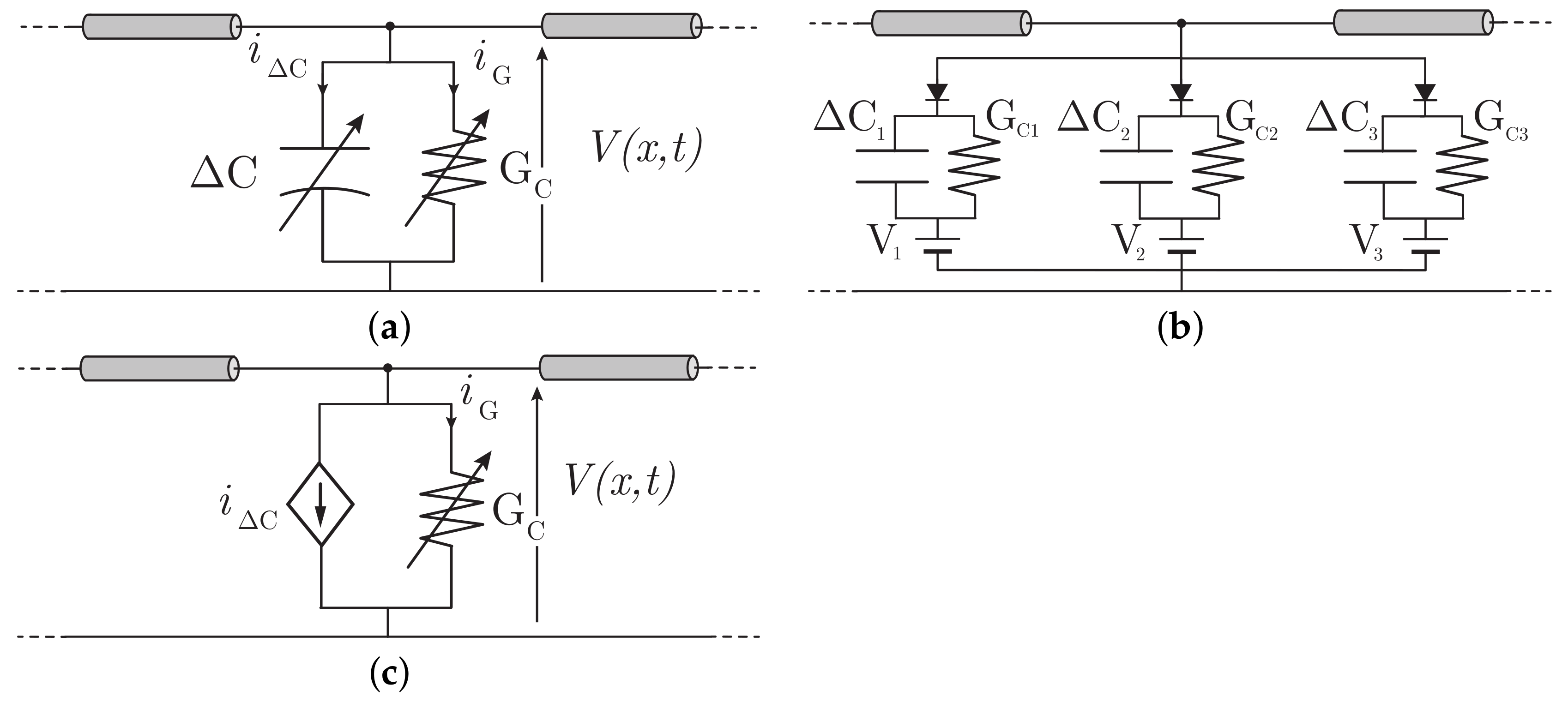
4.4. Circuit-Based Models

4.4.1. Hara and Umoto’s Model

Several models are based on the assumption that the p.u.l. corona losses $p^{\prime }$ can be computed through the following quadratic frequency-dependent relation originally proposed by Peek, and expressed in W/m [4]:

$$p^{\prime }\left(t\right)=\frac{\kappa }{\delta }\sqrt{\frac{r_0}{2h}}f{\left[v\left(t\right)-V_{\mathrm{inc}}\right]}^2,$$

(45)

where f is the frequency in Hz, $v\left(t\right)$ and $V_{\mathrm{inc}}$ are in V, $\delta$ is the air relative density, and $\kappa$ is a corona loss constant, expressed in s/($\mathsf{\Omega }$m), found from the analysis of experimental data.

Starting from (45), Hara and Umoto proposed to include the effect of corona in a finite-difference time-domain (FDTD) updating scheme by connecting in parallel two lumped non-linear voltage-dependent components along the line when the electric field $e_0\left(t\right)$ reaches the inception value $E_{\mathrm{inc}}$. The equivalent circuit is represented in Figure 6a; additional lumped shunt branches include the capacitance $\mathsf{\Delta }C$, modeling corona space-charge effect, and a conductance $G_{\mathrm{C}}$, accounting for additional corona losses. The expression for the currents drained by the branches, $i_{\mathsf{\Delta }C}$ and $i_{\mathrm{G}}$ respectively, were originally proposed in [68], and then recalled by Lee [69]:

$$\begin{array}{}\mathrm{(46a)}& i_{\mathsf{\Delta }C}=\mathsf{\Delta }C\frac{\mathrm{d}v\left(t\right)}{\mathrm{d}t}=2{\kappa }_{\mathrm{C}}\left[1-\frac{V_{\mathrm{inc}}}{v\left(t\right)}\right]\frac{\mathrm{d}v\left(t\right)}{\mathrm{d}t}\mathsf{\Delta }\ell \hfill \mathrm{(46b)}& i_{\mathrm{G}}=G_{\mathrm{C}}v\left(t\right)={\kappa }_{\mathrm{G}}{\left[1-\frac{V_{\mathrm{inc}}}{v\left(t\right)}\right]}^{2}v\left(t\right)\mathsf{\Delta }\ell ,\hfill \end{array}$$

with

$$\begin{array}{}\mathrm{(47a)}& \mathsf{\Delta }C=2{\kappa }_{\mathrm{C}}\left[1-\frac{V_{\mathrm{inc}}}{v\left(t\right)}\right]\mathsf{\Delta }\ell \hfill \mathrm{(47b)}& G_{\mathrm{C}}={\kappa }_{\mathrm{G}}{\left[1-\frac{V_{\mathrm{inc}}}{v\left(t\right)}\right]}^2\mathsf{\Delta }\ell .\hfill \end{array}$$

The factors ${\kappa }_{\mathrm{C}}$ and ${\kappa }_{\mathrm{G}}$ may be expressed as follows:

$${\kappa }_{\mathrm{C},\mathrm{G}}={\sigma }_{\mathrm{C},\mathrm{G}}\sqrt{\frac{r}{2h}}·{10}^{-11}$$

(48)

where ${\sigma }_{\mathrm{C}}$ is approximately in the range $15÷35$$\mathrm{F}/\mathrm{m}$, and ${\sigma }_{\mathrm{G}}$ (corona loss constant) is in the interval $5\times {10}^6÷20\times {10}^6$ $\mathrm{S}/\mathrm{m}$, depending on the configuration under study.

For sufficient accuracy, the distance between voltage nodes equipped with additional lumped corona branches should be less than $\mathsf{\Delta }\ell =70$ $\mathrm{m}$; indeed, a further increment in $\mathsf{\Delta }\ell$ would result in noticeable deviation from the benchmark experimental data [69].

4.4.2. Motoyama and Ametani’s Model

In order to avoid the non-linear components present in Hara and Umoto’s model, Motoyama and Ametani [70] proposed a further development. The expressions given in (47) for the lumped equivalent capacitance and conductance are replaced by three-levels piece-wise constant functions of the voltage $v\left(t\right)$, which are valid for $\mathrm{d}v/\mathrm{d}t>0$:

$$\mathsf{\Delta }C\left(v\right)=\left\{\begin{array}{cc}\mathsf{\Delta }{C}_1,\hfill & V_{\mathrm{inc}}\le v<2V_{\mathrm{inc}}\hfill \\ \mathsf{\Delta }{C}_1+\mathsf{\Delta }{C}_2,\hfill & 2V_{\mathrm{inc}}\le v<3V_{\mathrm{inc}}\hfill \\ \mathsf{\Delta }{C}_1+\mathsf{\Delta }{C}_2+\mathsf{\Delta }{C}_3,\hfill & v\ge 3V_{\mathrm{inc}},\hfill \end{array}\right.$$

(49)

and

$$G_{\mathrm{C}}\left(v\right)=\left\{\begin{array}{cc}{G}_{\mathrm{C}1},\hfill & V_{\mathrm{inc}}\le v<2V_{\mathrm{inc}}\hfill \\ G_{\mathrm{C}1}+G_{\mathrm{C}2},\hfill & 2V_{\mathrm{inc}}\le v<3V_{\mathrm{inc}}\hfill \\ G_{\mathrm{C}1}+G_{\mathrm{C}2}+G_{\mathrm{C}3},\hfill & v\ge 3V_{\mathrm{inc}},\hfill \end{array}\right.$$

(50)

where

$$\begin{array}{}\mathrm{(51a)}& \mathsf{\Delta }{C}_k=2{\kappa }_{\mathrm{C}}\left(1-\frac{V_{\mathrm{inc}}}{V_{\mathrm{inc}}+V_k}\right)\mathsf{\Delta }\ell \hfill \mathrm{(51b)}& G_{\mathrm{C}k}={\kappa }_{\mathrm{G}}{\left(1-\frac{V_{\mathrm{inc}}}{V_{\mathrm{inc}}+V_k}\right)}^2\mathsf{\Delta }\ell \hfill \end{array}$$

with $V_k=k{V}_{\mathrm{inc}}$, $k=$1, 2, 3.

The parameters ${\kappa }_{\mathrm{C}}$ and ${\kappa }_{\mathrm{G}}$ are given by expressions (48), in which ${\sigma }_{\mathrm{C}}$ ranges approximately between $2÷33$ F/m, and ${\sigma }_{\mathrm{G}}$ is in the interval $0.5\times {10}^6÷13\times {10}^6$ S/m. The proposed model may be easily embedded in any transients program, plugging the equivalent circuit in Figure 6b to selected voltage nodes; the model is claimed to be more practical with respect to Lee’s model: it should allow to plug lumped circuits for corona at larger intervals, even just at the poles for $\mathsf{\Delta }\ell$ in the range $350÷450$ m, still holding accuracy [70].

4.4.3. Maccioni-Araneo et al. Model

The model refers to a single conductor, and introduces a couple of lumped additional shunt branches [71] as shown in Figure 6c: the first branch consists in the voltage-controlled current generator $i_{\mathsf{\Delta }\mathrm{C}}\left(t\right)$ simulating the increment in the capacitive current; the second branch is represented by a non-linear conductance $G_{\mathsf{\Delta }\mathrm{C}}\left(t\right)$, accounting for corona losses. As the voltage $v\left(t\right)$ reaches $V_{\mathrm{inc}}$, the voltage-controlled current generator is turned on, fictitiously reproducing the increase in capacitance $\mathsf{\Delta }C\left(t\right)$ due to corona. As the voltage starts to decrease, it is turned off so that $\mathsf{\Delta }C\left(t\right)=0$ on the descending branch of the q-v curve, and the conductor charge depends linearly on the voltage through $C_{\mathrm{geo}}^{\prime }\mathsf{\Delta }\ell$.

Following the theory of the physics-based models, when $\mathrm{d}v/\mathrm{d}t>0$, $\mathsf{\Delta }C\left(t\right)$ is computed as the following:

$$\mathsf{\Delta }C\left(t\right)=2\pi {\epsilon }_0\left[\frac{1}{ln\frac{2h}{r_{\mathrm{c}}\left(t\right)}}-\frac{1}{ln\frac{2h}{r_0}}\right]\mathsf{\Delta }\ell ,$$

(52)

where the time dependent radius $r_{\mathrm{c}}\left(t\right)$ is computed through the following non-linear equation:

$$v\left(t\right)=r_{\mathrm{c}}\left(t\right)E_{\mathrm{inc}}ln\left[\frac{2h}{r_{\mathrm{c}}\left(t\right)}\right].$$

(53)

The current generator $i_{\mathsf{\Delta }\mathrm{C}}\left(t\right)=\mathrm{d}\left[\mathsf{\Delta }C\left(t\right)v\left(t\right)\right]/\mathrm{d}t$ is given by the following:

$$i_{\mathsf{\Delta }\mathrm{C}}\left(t\right)=\left\{\begin{array}{cc}0,\hfill & v\left(t\right)<V_{\mathrm{inc}}\mathrm{or}\mathrm{d}v/\mathrm{d}t<0\hfill \\ v\left(t\right)\frac{\mathrm{d}\mathsf{\Delta }C\left(t\right)}{\mathrm{d}t}+\mathsf{\Delta }C\left(t\right)\frac{\mathrm{d}v\left(t\right)}{\mathrm{d}t},\hfill & v\left(t\right)\ge V_{\mathrm{inc}}\mathrm{and}\mathrm{d}v/\mathrm{d}t>0\hfill \end{array}\right.$$

(54)

Equations (52)–(54) can be easily inserted into any FDTD scheme.

The value of the lumped equivalent conductance $G_{\mathrm{C}}\left(v\right)$ is computed according to (47b) [69] for $v\left(t\right)\ge V_{\mathrm{inc}}$ and $\mathrm{d}v/\mathrm{d}t>0$. Once the voltage applied to the conductor has reached its maximum value $V_{\max }$ and begins to decrease, the conductance $G_{\mathrm{C}}$ is kept connected to the line, according to [89]; however, the value of $G_{\mathrm{C}}$ is no longer voltage-dependent, but is assumed to be constant and equal to the value attained by (47b) when the corona radius has reached its maximum value $r=r_{max}$.

With reference to (53), the main simplifying hypothesis adopted by this model consists in assuming the corona sheath to be conductive enough so that the voltage drop across the ionized area may be disregarded; hence, the potential $v\left(t\right)$ is intended to be measured at the outer surface of the space-charge region, $\mathit{not}$ at $r_0$ on the conductor surface.

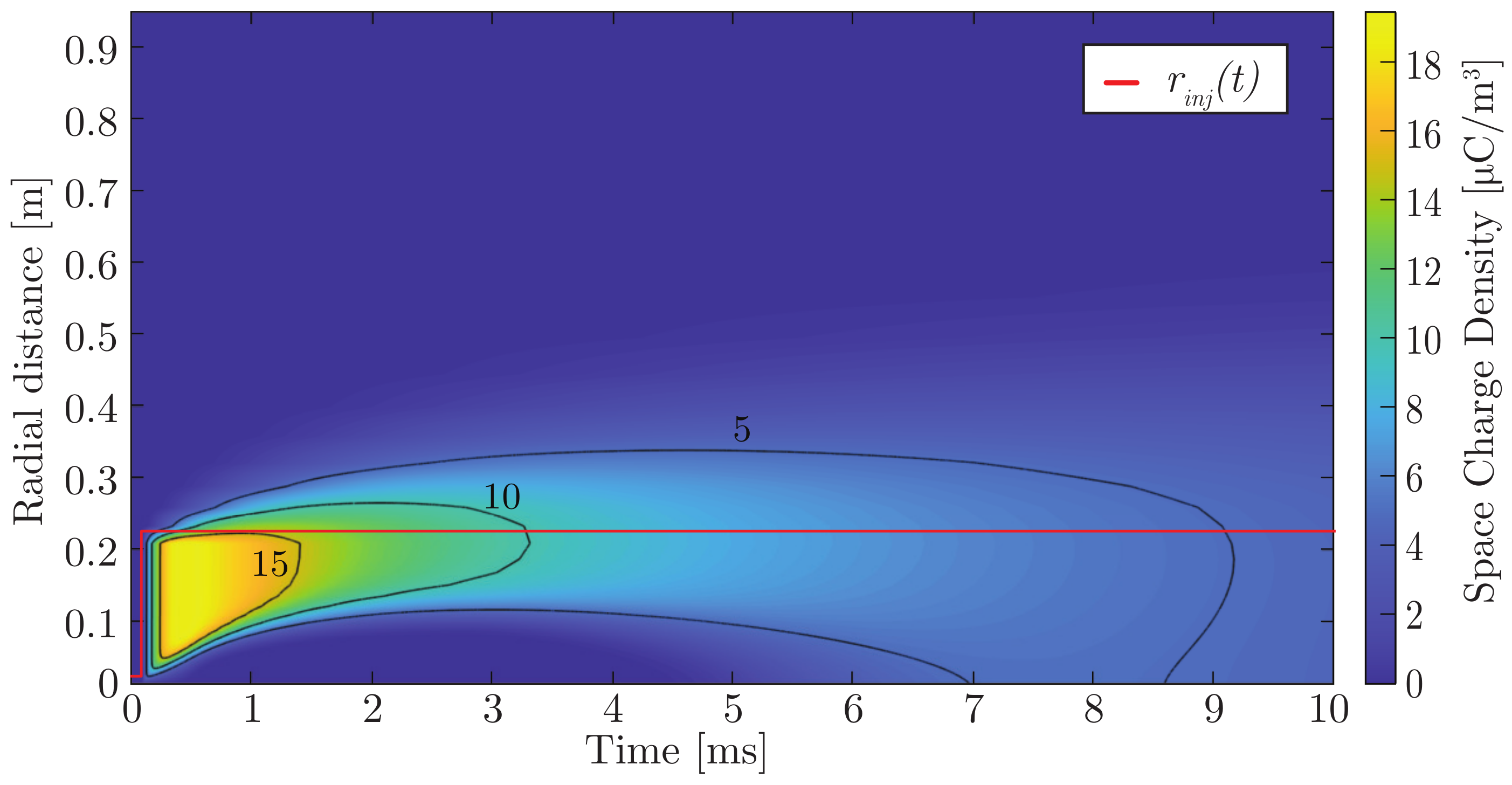
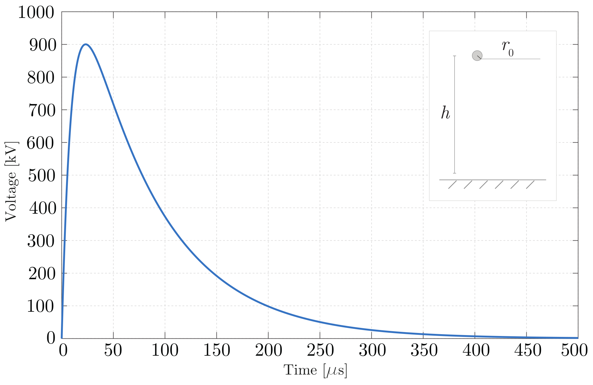
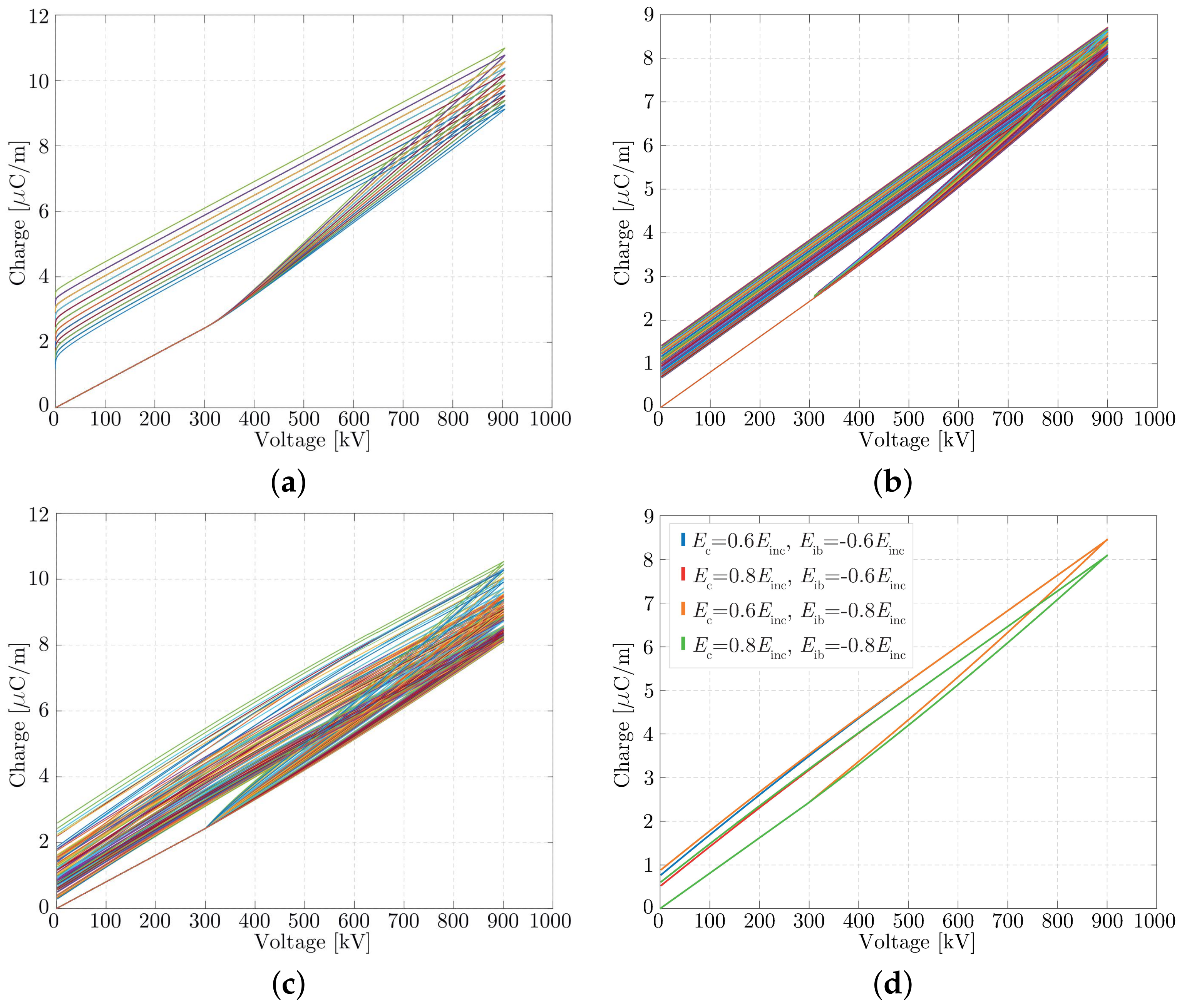
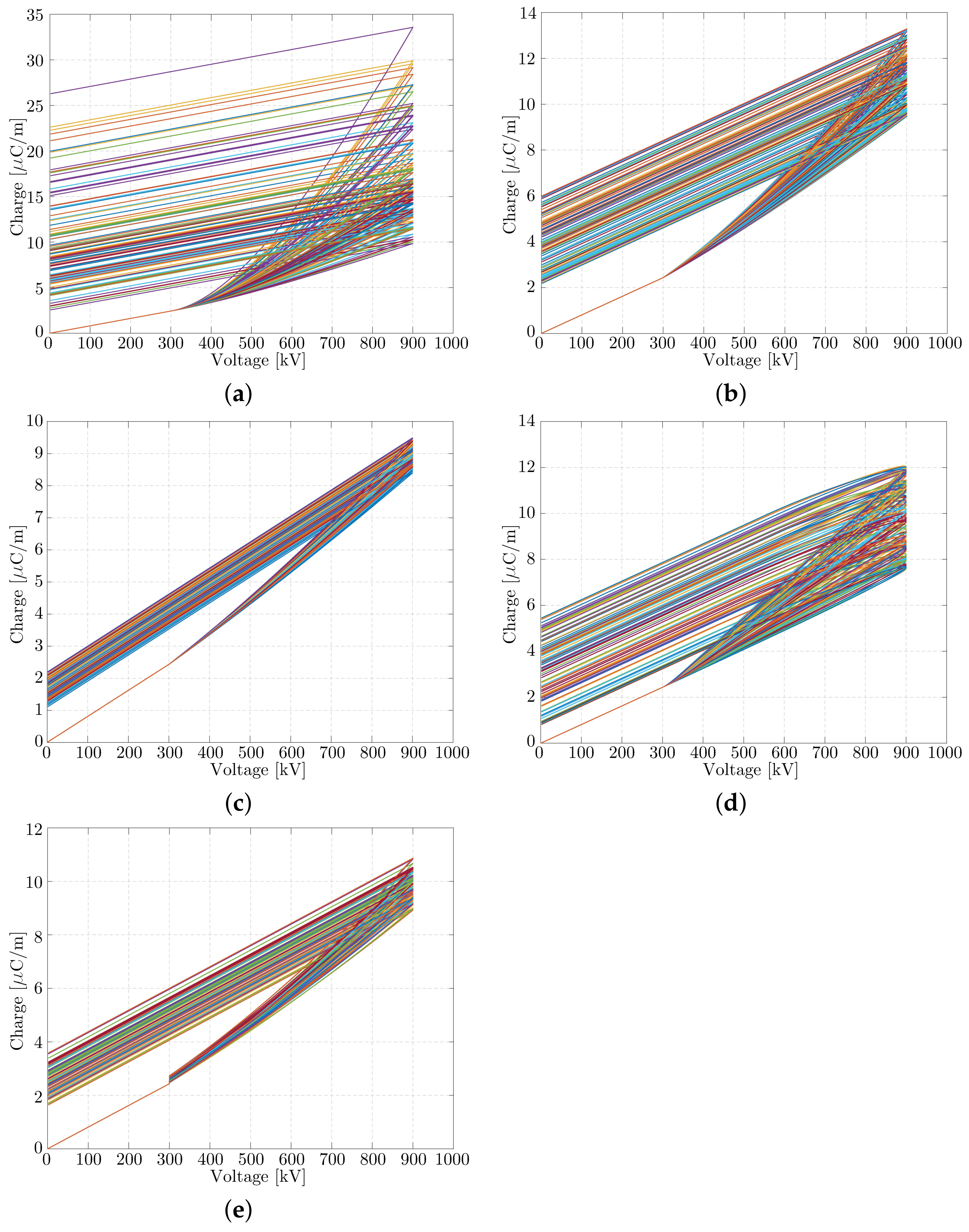
5. Results: Comparison of the Models Responses to the Variability of Input Parameters

Table 5. Comparison of the models.

	Number of Input Parameters	Input Parameters	Applied Voltage Waveform
Correia de Barros	4	$r_{\mathrm{s}}$, $v_{\mathrm{st}}$, ${\tau }_{\mathrm{st}}$, ${\tau }_0$	Impulse and AC steady-state voltage
Malik et al.	2	$\alpha$, $\tau$	Impulse voltage
Cooray et al.	3	$E_{\mathrm{c}}$, $E_{\mathrm{ib}}$, ${\tau }_{\mathrm{d}}$	Impulse voltage
Inoue	2	$\alpha$, ${\sigma }_{\kappa }$	Impulse voltage
Gary et al.	1	B	Impulse voltage
Podporkin and Sivaev	3	${\kappa }_1$, ${\kappa }_2$, a	Impulse voltage
Suliciu et al.	4	$C_1^{\prime }$, $C_2^{\prime }$, $K_1$, $K_2$	Impulse voltage
CIGRÉ	2	K, $C_{\mathrm{I}}^{\prime }$	Impulse voltage
Hara and Umoto	2	${\sigma }_{\mathrm{C}}$, ${\sigma }_{\mathrm{G}}$	Impulse voltage
Motoyama and Ametani	2	${\sigma }_{\mathrm{C}}$, ${\sigma }_{\mathrm{G}}$	Impulse voltage
Maccioni, Araneo et al.	1	${\sigma }_{\mathrm{G}}$	Impulse voltage

is provided to compare the models reviewed here in terms of the number of required input parameters, and applicability with respect to the voltage source applied to the conductor under test. As to their validity with respect to the voltage source, all the models should be exploited when a unipolar waveform is applied to the conductor, except for the model by Correia de Barros, which is suitable for studies involving any voltage waveform, both impulsive and AC steady-state (due to the modeling of the drift of negative and positive charges). In this section, curves are provided to address the influence of the parameters required by each model on the shape of the final q-v curves. The reference voltage impulse displayed in Figure 7 is applied to a reference conductor (whose characteristics are summarized in

Table 6. Parameters of the reference configuration in the inset of Figure 7.

h	7.5 m
$r_0$	1.57 cm
$V_{\mathrm{inc}}$	300 kV

):

$$v\left(t\right)=\frac{V_{\max }}{\eta }\left[exp\left(\frac{-t}{{\tau }_2}\right)-exp\left(\frac{-t}{{\tau }_1}\right)\right],$$

(55)

where ${\tau }_1=10$ $\mathsf{\mu }$s, ${\tau }_2=75$ $\mathsf{\mu }$s, and $\eta =0.636$ is the amplitude correction factor. To this aim, the voltage maximum value is chosen to be equal to $V_{\max }=3V_{\mathrm{inc}}$, $V_{\mathrm{inc}}$ for the reference conductor being computed, according to Peek’s formula (1) since the validity of the formula proposed by Mikropoulos and Zagkanas [37] is limited to coaxial configurations, and the criterion proposed by Olsen and Yamazaki applies to power frequencies.

In the following sections, we address the variability of the hysteretic q-v loops computed by the different approaches with respect to the input parameters required by the models. In particular, for a model depending on $n_p$ input parameters, an $n_p$-dimensional finite region of space is defined, where the $n_p$ parameters may vary in well-defined ranges of admissible values; q-v curves are displayed corresponding to one hundred points of this space, i.e., to one hundred different combinations of the input parameters, the values of which are randomly extracted from a uniform distribution in their variability range.

5.1. Sensitivity Curves for Physics-Based Models

The hysteretic curves given by the physics-based models are displayed in Figure 8.

Figure 8a shows q-v loops computed by Correia de Barros’ model in Section 4.2.1. The input parameters range in the following intervals (derived from data found in the literature): $r_{\mathrm{s}}\in \left[10·r_0,30·r_0\right]$, $v_{\mathrm{st}}\in \left[0.3\times {10}^6,1.1\times {10}^6\right]$, ${\tau }_{\mathrm{st}}\in \left[0.5,0.7\right]$ $\mathsf{\mu }$s, ${\tau }_0=0.5$ $\mathsf{\mu }$s.

The results of Malik’s model are in Figure 8b. The input parameters required by the model, i.e., $\tau$ and $\alpha$, range between $0.1÷0.5$$\mathsf{\mu }$s and $0.5÷0.9$, respectively. The model does not show significant dependence on the input parameters; their impact may be noticed at the inception. In fact, the different time delays $\tau$ result in slight variations in the location of the discontinuity in the q-v loops at the inception. Furthermore, lower values of $\alpha$ result in a faster growth of the equivalent external radius; hence, the slope of the rising branch in Figure 8b is more pronounced, enlarging the total loop area. Charge-voltage curves computed by Cooray’s model are shown in Figure 8c. The variability ranges assumed for the input parameters are: $E_{\mathrm{c}}\in \left[0.2·E_{\mathrm{inc}},0.8·E_{\mathrm{inc}}\right]$, $E_{\mathrm{ib}}\in \left[-0.8·E_{\mathrm{inc}},-0.2·E_{\mathrm{inc}}\right]$, ${\tau }_{\mathrm{d}}=0.5$ $\mathsf{\mu }$s. The slope of the ascending branch of the loops, after the inception, is related to $E_{\mathrm{c}}$: values of $E_{\mathrm{c}}$ closer to (much smaller than) $E_{\mathrm{inc}}$ result in a slow (fast) growth of the charge with respect to the voltage. If the electric field on the conductor surface reaches the value $E_{\mathrm{ib}}$ at the voltage tail, the charge decay will be faster, with lower values of residual p.u.l. charge. In fact, the descending branch will deviate from the expected linear decay with slope equal to $C_{\mathrm{geo}}^{\prime }$ (see Figure 8d).

As to the shape of the hysteretic curves, the models result in different shapes; with reference to Malik’s model, the loops are tight and of definite shape, predicting the maximum p.u.l. charge values to be lower with respect to results by Cooray and Correia de Barros, which, on the contrary, are in good agreement.

Comparison of the descending branches of the curves reveals some differences. The constant value of the p.u.l. capacitance assumed by Malik, equal to $C_{\mathrm{geo}}^{\prime }$, results in the constant slope of the corresponding branch. Instead, Cooray’s curves show more pronounced slopes for $\mathrm{d}v/\mathrm{d}t<0$, due to the progressive accumulation of negative p.u.l. charge on the conductor surface, and to the subsequent inception of back corona (depending on the value of $E_{\mathrm{ib}}$).

Correia de Barros’ results are computed for a larger time-window, up to 1 ms, in order to properly show the curvature of the descending branches for $v\left(t\right)\to 0$. If the other models present a residual p.u.l. charge caused by the applied voltage amplitude and time derivative approaching zero, $q^{\prime }\left(t\right)$ vanishes in Figure 8a for $v\left(t\right)\to 0$ and $t\to \infty$, due to the gradual drift of residual charged particles surrounding the conductor.

5.2. Sensitivity Curves for Empirical Models

Figure 9 collects the responses to the applied voltage source computed by means of the empirical models in Section 4.3. Sensitivity studies are conducted by choosing some variability ranges for the parameters required by the models (which should be set by fitting experimental data), from analogy with values adopted in previous applications in the literature (if available), or arbitrarily.

Inoue’s model gives rise to the widest range of variability of the output curves; hence, its predictive capability is questionable, and comparison with measured data is essential for the suitable tuning of the input parameters and computation of reliable results. The curves in Figure 9a are obtained for $\alpha \in \left[2,2.1\right]$ and ${\sigma }_{\kappa }\in \left[100,450\right]$ pF/m (similar values are adopted in [61] for the first branch of the q-v loop after the inception). The product ${\sigma }_{\kappa }·\alpha$ determines the slope of the non-linear sections.

Gary’s approach requires the choice of the parameter B to fit experimental data (see Equation (36) for original values by Gary). In order to address the model dependence on B, curves in Figure 9b were computed with $B\in 1.23÷1.55$, i.e., in the range defined by values in Equation (36), chosen as limiting values of the interval. Wider loops correspond to larger values of B.

Figure 9c presents the curves computed through the approach by Sivaev and Podporkin. Since ${\kappa }_1=1.17$ and ${\kappa }_2=0.87$ should be of practical use for $0.5<r_0<3$ cm and $10<h<30$ m [63], here, we adopt limited (arbitrary and heuristic) ranges of variability to account for the different height of the conductor $h=7.5\mathrm{m}<10$ m): ${\kappa }_1\in \left[1.1,1.2\right]$, ${\kappa }_2\in \left[0.8,0.9\right]$, while a is in the interval $0.036÷0.08$.

As for Suliciu’s model, the following set of input parameters was chosen: $C_1^{\prime }\in \left[C_{\mathrm{geo}}^{\prime },2C_{\mathrm{geo}}^{\prime }\right]$, $C_2^{\prime }\in \left[C_{\mathrm{geo}}^{\prime },4C_{\mathrm{geo}}^{\prime }\right]$ ensuring $C_2^{\prime }>C_1^{\prime }$, $K_1\in \left[0.5,5\right]$ MHz, and $K_2\in \left[0.5,5\right]$ kHz. The output curves show a characteristic shape; in particular, the maximum p.u.l. charge value may not correspond to the maximum applied voltage. This is due to the fact that the capacitive current derived toward the ground depends not only on the voltage time-derivative, but also on the voltage instantaneous value (Equation (41)).

Sensitivity curves computed by the Cigré model with respect to $C_{\mathrm{I}}^{\prime }$, K are shown in Figure 9e. Considering the values of K in [66] corresponding to the diameter of the reference conductor, q-v loops are displayed for $K\in \left[2.5\times {10}^{-6},5\times {10}^{-6}\right]$ pF/(V·m), while the value of $C_{\mathrm{I}}^{\prime }<1$ pF/m [66] is chosen between 0.1÷1 pF/m. Growing values of $C_{\mathrm{I}}^{\prime }$ introduce harsher step-like discontinuities at the inception voltage, i.e., for $v\approx 300$ kV; instead, larger values of K enhance the rate of rise of the non-linear branch of the curves.

5.3. Sensitivity Curves for Circuit-Based Models

In Section 4.4.1 and Section 4.4.2, the parameter denoted with ${\sigma }_{\mathrm{C}}$ is responsible for variation of the capacitance computed by the corresponding models. In Figure 10b,c, we present the curves computed by the models of Hara–Umoto and Motoyama–Ametani, respectively, with ${\sigma }_{\mathrm{C}}$ ranging in the interval $15÷35$ F/m (from values adopted in [69], in good agreement with [70]). Both models are strongly dependent on the input parameter, as may be deduced by the noticeable variability in the displayed curves. Greater values of ${\sigma }_{\mathrm{C}}$ correspond to larger q-v loops.

The hysteretic curves in Figure 10b are wider than the curves in Figure 10a. This is due to the simplified approach proposed by Motoyama and Ametani (see Section 4.4.2). In fact, for the voltage intervals $V_{\mathrm{inc}}\le v\left(t\right)<2V_{\mathrm{inc}}$ and $2V_{\mathrm{inc}}\le v\left(t\right)<3V_{\mathrm{inc}}$, the piece-wise constant capacitance defined by Motoyama and Ametani exceeds the values computed by Hara and Umoto’s approach.

The single parameter required by the model of Maccioni–Araneo et al. is ${\sigma }_{\mathrm{G}}$, which defines the conductance accounting for the corona losses in its equivalent circuit representation. Instead, the capacitive current, denoted with $i_{\mathsf{\Delta }\mathrm{C}}$ in Section 4.4.3, only depends on the geometrical features of the configuration under study and on the conductor voltage. Hence, the total charge corresponding to the applied voltage (which is derived by integrating the additional corona capacitive current $i_{\mathsf{\Delta }\mathrm{C}}$ with respect to time and accounting for the instantaneous electrostatic charge) is displayed in Figure 10c (the independence of any input parameters results in a single q-v loop).

6. Discussion

The available methods for the computation of the corona onset voltage for DC and AC applications show good agreement with the measured values [90] and produce results with differences up to 4% [91], which are acceptable for the estimation of conductors’ surface voltage gradients. Inception voltages computed using Peek’s equation agree well, provided that an appropriate value of the irregularity factor m is included [92]. Despite its simplicity, Peek’s equation, which is largely used for engineering purpose, strongly depends on the correct choice of m, and this choice is not trivial since m varies significantly [38] with the conductors geometry, surface state, and weather conditions. Hence, it is necessary to derive a suitable value from past experience and/or available measurements.

Moving to stranded conductors—being that the electrical field at the tip of each strand is about 14% higher than the field on the surface of a smooth cylindrical conductor of the same diameter [91]—and bundles, the situation is even less trivial. Usually, engineers refer to an equivalent conductor, which approximates the bundle [93]. However, the surface electric field of the equivalent is lower than that of the bundle, so further corrections are needed when calculating the onset voltage. Despite the large literature, difficulties to correctly quantify the corona onset voltage still arise in these cases.

Successively, we have discussed and compared the reviewed models in terms of their advantageous and disadvantageous characteristics. A practical overview on the considerations to be made when choosing a specific model for implementation is presented in

Table 7. Features of the reviewed models.

	Advantages	Disadvantages
Correia de Barros	· Accurate physical modelling of the phenomenon; · Drift of the charges is simulated.	· Structured coding is necessary; · Requires longer computation times; · Several input parameters are required.
Malik	· Simple implementation.	· Predicts narrow q-v curves; · Limited versatility when fitting experimental data.
Cooray	· Simple implementation; · Implementation of back corona in the descending branch of q-v loops.	· Predicts an instantaneous q-v relation (unlike other physics-based models).
Inoue	· Simple implementation; · Versatility when fitting experimental data.	· Strong dependence on the input parameters: questionable predicting capability; · No distinction between positive and negative corona.
Gary et al.	· Simple implementation · Distinction between positive and negative corona.	· Predicts the discontinuity of the dynamic capacitance at the corona inception.
Podporkin and Sivaev	· Simple implementation.	· Predicts a step discontinuity of the dynamic capacitance at the corona inception.
Suliciu	· Allows to model q-v loops presenting non-simultaneous maximum values of charge and voltage.	· Several input parameters are required.
CIGRÉ	· Simple implementation.	· Predicts the discontinuity of the dynamic capacitance at the corona inception.
Hara and Umoto	· Trivial implementation in programs for electro-magnetic transient studies.	· Less accurate representation of corona as a distributedphenomenon.
Motoyama and Ametani	· Trivial implementation; · Limited computational burden.	· Excessive simplification of the non-linear phenomenon, through constant-valued additional $\mathsf{\Delta }C$; · Less accurate representation of corona as a distributed phenomenon.
Maccioni, Araneo et al.	· Simple implementation in programs for electro-magnetic transient studies.	· Computed q-v curves have fixed shape: they cannot be adjusted to better match measured data; · Less accurate representation of corona as a distributed phenomenon.

. Only Correia de Barros’ approach models the drift of the charged particles. Hence, it allows to consider the dynamic of the p.u.l. charge approaching zero for large simulation times and decaying values of the applied voltage, at the cost of a heavier computational burden. On the contrary, Malik and Cooray’s models, being based on a macroscopic approximation of the physical phenomenon, are easier to implement. In particular, since the shape of the q-v loops computed through Malik’s model is narrower and hardly dependent on the input parameters (see Figure 8b), the model may not be suitable to fit differently shaped measured q-v curves.

Only Inoue’s model does not predict discontinuities in the p.u.l. capacitance value at corona inception; with reference to Suliciu’s approach, a discontinuity may be introduced depending on the values attributed to ${\tilde{v}}_j$ ($j=1,2$). The introduction of a harsh discontinuity of the p.u.l. dynamic capacitance (i.e., an abrupt change in the propagation velocity of traveling waves) requires careful implementation in FDTD approaches in order to avoid numerical instability [51].

Finally, the implementation of circuit-based models requires a compromise to be made between the simplicity of plugging a limited number of shunt branches to the TL under study and the accuracy in modeling the corona effect as a non-lumped phenomenon.

7. Conclusions

This paper reviews and summarizes the main phenomena involved with corona discharge: microscopic and macroscopic dynamics, electric field distribution at the inception. Special attention is devoted to the influence of corona discharge on the p.u.l. parameters of overhead transmission lines, referring to the additional power losses and the enhanced capacitive behavior, which are addressed in the second part of the paper. This point is addressed through a comprehensive and critical review of a wide selection of models available in the literature for the simulation of the relation between p.u.l. charge and voltage.

With respect to a chosen voltage source applied to a reference conductor, the corona models are implemented to compute the charge–voltage hysteretic loops and evaluate the models’ sensitivity to variations in the required set of input parameters.

Most of the models display a remarkable dependence on the input parameters, which may be properly adjusted in order to reproduce charge–voltage measured loops. However, due to this tunability feature, the models are suitable for reproducing experimental data rather than for predictive studies of the electrical behavior of transmission lines.

Further updates in research are necessary to study approaches of general applicability with limited dependence on additional parameters, which may be exploited to assess the influence of corona discharge on propagation phenomena along transmission lines regardless the availability of pre-existing measured values of charge and voltage in the analyzed configurations.

References

1. Laplante, P.A. Electrical Engineering Dictionary; CRC Press LLC: Boca Raton, FL, USA, 2000. [Google Scholar]
2. Gallimberti, I. The mechanism of the long spark formation. J. Phys. Colloq. 1979, 40, C7-193. [Google Scholar]
3. Faraday, M. VIII. Experimental Researches in Electricity—Thirteenth Series; Philosophical Transactions of the Royal Society of London: London, UK, 1838; pp. 125–168. [Google Scholar]
4. Peek, F.W. The law of corona and the dielectric strength of air. Proc. Am. Inst. Electr. Eng. 1911, 30, 1485–1561. [Google Scholar]
5. Peek, F.W. The law of corona and dielectric strength of air—II. Proc. Am. Inst. Electr. Eng. 1912, 31, 1085–1126. [Google Scholar] [CrossRef]
6. Peek, F.W. Dielectric Phenomena in High Voltage Engineering; McGraw-Hill Book Company, Incorporated: London, UK, 1920. [Google Scholar]
7. Rizk, F.A.; Trinh, G.N. High Voltage Engineering; CRC Press: Boca Raton, FL, USA, 2018. [Google Scholar]
8. Goldman, M.; Goldman, A.; Sigmond, R. The corona discharge, its properties and specific uses. Pure Appl. Chem. 1985, 57, 1353–1362. [Google Scholar] [CrossRef] [Green Version]
9. Gary, C.; Moreau, M. L’Effet de Couronne en Tension Alternative; Collection de la Direction des Etudes et Recherches d’Electricité de France: Paris, France, 1976. [Google Scholar]
10. Riba, J.R.; Larzelere, W.; Rickmann, J. Voltage correction factors for air-insulated transmission lines operating in high-altitude regions to limit corona activity: A review. Energies 2018, 11, 1908. [Google Scholar] [CrossRef] [Green Version]
11. Yamazaki, K.; Olsen, R.G. Application of a corona onset criterion to calculation of corona onset voltage of stranded conductors. IEEE Trans. Dielectr. Electr. Insul. 2004, 11, 674–680. [Google Scholar]
12. Bousiou, E.I.; Mikropoulos, P.N.; Zagkanas, V.N. Experimental Investigation of the Overvoltage Steepness Effects on Corona Inception Characteristics. In The International Symposium on High Voltage Engineering; Springer: Cham, Switzerland, 2019; pp. 1413–1422. [Google Scholar]
13. Lings, R. EPRI AC Transmission Line Reference Book: 200 KV and Above, 3rd ed.; Electric Power Research Institute: Palo Alto, CA, USA, 2005. [Google Scholar]
14. Wagner, C.F.; Lloyd, B.L. Effects of corona on traveling waves. Electr. Eng. 1955, 74, 1071. [Google Scholar] [CrossRef]
15. Krzewiński, S.; Frącz, P.; Urbaniec, I.; Turba, T. Comparative analysis of optical signals emitted by corona on a laboratory model of transmission lines made of various materials. J. Spectrosc. 2017, 2017, 8423797. [Google Scholar]
16. Tyler, N.J.; Stokkan, K.A.; Hogg, C.R.; Nellemann, C.; Vistnes, A.I. Cryptic impact: Visual detection of corona light and avoidance of power lines by reindeer. Wildl. Soc. Bull. 2016, 40, 50–58. [Google Scholar] [CrossRef] [Green Version]
17. Engel, Z.; Wszołek, T. Audible noise of transmission lines caused by the corona effect: Analysis, modelling, prediction. Appl. Acoust. 1996, 47, 149–163. [Google Scholar] [CrossRef]
18. IEEE Std 430-2017. IEEE Standard Procedures for the Measurement of Radio Noise from Overhead Power Lines and Substations; Revision of IEEE Std 430-1986; IEEE Standards Association: Piscataway, NJ, USA, 2017; pp. 1–34. [Google Scholar]
19. IEC. CISPR TR 18-1 Radio Interference Characteristics of Overhead Power Lines and High-Voltage Equipment—Part 1: Description of Phenomena; IEC: Geneva, Switzerland, 2017. [Google Scholar]
20. CIGRE. Guide for Measurement of Radio Frequency Interference from HV and MV Substations; CIGRE Technical Brochure 391; CIGRE: Paris, France, 2009. [Google Scholar]
21. Liu, Z. Ultra-High Voltage AC/DC Grids; Academic Press: Cambridge, MA, USA, 2014. [Google Scholar]
22. Donini, A.; Spezie, R.; Cortina, R.; Piana, E.A.; Turri, R. Accurate prediction of the corona noise produced by overhead transmission lines. In Proceedings of the AEIT International Annual Conference, Capri, Italy, 5–7 October 2016; pp. 1–6. [Google Scholar]
23. Adamiak, K.; Atrazhev, V.; Atten, P. Corona discharge in the hyperbolic point-plane configuration: Direct ionization criterion versus an approximate formulations. IEEE Trans. Dielectr. Electr. Insul. 2005, 12, 1015–1024. [Google Scholar] [CrossRef]
24. Townsend, J.S. Electricity in gases; Clarendon Press: New York, NY, USA, 1915. [Google Scholar]
25. Georghiou, G.E.; Papadakis, A.; Morrow, R.; Metaxas, A. Numerical modelling of atmospheric pressure gas discharges leading to plasma production. J. Phys. Appl. Phys. 2005, 38, R303. [Google Scholar] [CrossRef]
26. Wadhwa, C. High Voltage Engineering; New Age International: New Delhi, India, 2006. [Google Scholar]
27. Raizer, Y.P.; Allen, J.E. Gas Discharge Physics; Springer: Berlin, Germany, 1997; Volume 2. [Google Scholar]
28. Giao, T.N.; Jordan, J.B. Modes of corona discharges in air. IEEE Trans. Power App. Syst. 1968, 5, 1207–1215. [Google Scholar] [CrossRef]
29. Bousiou, E.I.; Mikropoulos, P.N.; Zagkanas, V.N. Experimental investigation of negative DC corona on conductor bundles: A comparison with positive corona. In Proceedings of the 2017 52nd International Universities Power Engineering Conference (UPEC), Heraklion, Greece, 28–31 August 2017; pp. 1–5. [Google Scholar]
30. Mikropoulos, P.; Zagkanas, V.; Koustoulidis, T. Experimental investigation of DC corona on stranded conductors under variable air density. In Proceedings of the 2012 47th International Universities Power Engineering Conference (UPEC), Uxbridge, UK, 4–7 September 2012; pp. 1–6. [Google Scholar]
31. CIGRE. Addendum to Doc. 20: Interferences Produced by Corona Effect of Electric Systems; CIGRE: Paris, France, 1966. [Google Scholar]
32. Loeb, L.B. Electrical Coronas, Their Basic Physical Mechanisms; University of California Press: Berkeley, CA, USA, 1965. [Google Scholar]
33. Abdel-Salam, M. High-Voltage Engineering: Theory and Practice, Revised and Expanded; CRC Press: Boca Raton, FL, USA, 2018. [Google Scholar]
34. Baldo, G.; Gallimberti, I.; Garcia, H.; Hutzler, B.; Jouaire, J.; Simon, M. Breakdown phenomena of long gaps under switching impulse conditions influence of distance and voltage level. IEEE Trans. Power App. Syst. 1975, 94, 1131–1140. [Google Scholar] [CrossRef]
35. Correia de Barros, M.T. Efeito Coroa em Linhas de Transporte de Energia. Ph.D. Thesis, IST-Tecnical University of Lisbon, Lisbon, Portugal, 1985. [Google Scholar]
36. Maruvada, P.S.; Menemenlis, H.; Malewski, R. Corona characteristics of conductor bundles under impulse voltages. IEEE Trans. Power App. Syst. 1977, 96, 102–115. [Google Scholar] [CrossRef]
37. Mikropoulos, P.N.; Zagkanas, V.N. Impulse corona inception in the coaxial cylindrical electrode arrangement in air: Effects of the steepness of the applied voltage. In Proceedings of the 18th International Symposium on High Voltage Engineering, Seoul, Korea, 25–30 August 2013. [Google Scholar]
38. Bousiou, E.I.; Mikropoulos, P.N.; Zagkanas, V.N. Corona inception field of typical overhead line conductors under variable atmospheric conditions. Electr. Power Syst. Res. 2020, 178, 106032. [Google Scholar] [CrossRef]
39. Mikropoulos, P.N.; Zagkanas, V.N. Threshold inception conditions for positive DC corona in the coaxial cylindrical electrode arrangement under variable atmospheric conditions. IEEE Trans. Dielectr. Electr. Insul. 2015, 22, 278–286. [Google Scholar] [CrossRef]
40. Maruvada, P.S.; Janischewskyj, W. DC corona on smooth conductors in air. Steady-state analysis of the ionisation layer. Proc. Inst. Electr. Eng. 1969, 116, 161–166. [Google Scholar]
41. Baker, A.; Comber, M.; Ottosen, K. Investigation of the corona performance of conductor bundles for 800-kV transmission. IEEE Trans. Power App. Syst. 1975, 94, 1117–1130. [Google Scholar] [CrossRef]
42. Zhang, X.; Zhang, Y. Experimental investigation and modeling of corona characteristics under lightning impulses. J. Electrost. 2017, 90, 85–90. [Google Scholar] [CrossRef]
43. Stone, L.N. EHV single and twin bundle conductors-influence of conductor diameter and strand diameter on radio influence voltage and corona initiation voltage. Trans. Am. Inst. Electr. Eng. Part III Power Appar. Syst. 1959, 78, 1434–1438. [Google Scholar] [CrossRef]
44. El-Bahy, M.M.; Abouelsaad, M.; Abdel-Gawad, N.; Badawi, M.; El-Bahy, M.M.; Abouelsaad, M.; Abdel-Gawad, N.; Badawi, M. Onset voltage of negative corona on stranded conductors. J. Phys. D Appl. Phys. 2007, 40, 3094. [Google Scholar] [CrossRef]
45. Abou-Seada, M.S. Digital Computer Calculation of Corona Thresholds in Nonuniform Fields. Ph.D. Thesis, Iowa State University, Ames, IA, USA, 1970. [Google Scholar]
46. Bousiou, E.I.; Mikropoulos, P.N.; Zagkanas, V.N. Experimental investigation of positive DC corona on conductor bundles. In Proceedings of the 2016 51st International Universities Power Engineering Conference (UPEC), Coimbra, Portugal, 6–9 September 2016; pp. 1–5. [Google Scholar]
47. Maruvada, P.S. A survey of methods for calculating transmission line conductor surface voltage gradients. IEEE Trans. Power App. Syst. 1979, 6, 1996–2014. [Google Scholar]
48. Alessandrini, V.; Fanchiotti, H.; Canal, C.G.; Vucetich, H. Exact solution of electrostatic problem for a system of parallel cylindrical conductors. J. Appl. Phys. 1974, 45, 3649–3661. [Google Scholar] [CrossRef]
49. Durbin, P.A.; Turyn, L. Analysis of the positive DC corona between coaxial cylinders. J. Phys. Appl. Phys. 1987, 20, 1490–1495. [Google Scholar] [CrossRef]
50. Monrolin, N.; Praud, O.; Plouraboué, F. Revisiting the positive DC corona discharge theory: Beyond Peek’s and Townsend’s law. Phys. Plasmas 2018, 25, 063503. [Google Scholar] [CrossRef] [Green Version]
51. Stracqualursi, E.; Araneo, R.; Andreotti, A. The Impact of Different Corona Models on FD Algorithms for the Solution of Multiconductor Transmission Lines Equations. High Volt. 2021, 1–14. [Google Scholar] [CrossRef]
52. Correia de Barros, M.T. Identification of the capacitance coefficients of multiphase transmission lines exhibiting corona under transient conditions. IEEE Trans. Power Del. 1995, 10, 1642–1648. [Google Scholar] [CrossRef]
53. De Jesus, C.; Correia de Barros, M.T. Modelling of corona dynamics for surge propagation studies. IEEE Trans. Power Del. 1994, 9, 1564–1569. [Google Scholar] [CrossRef]
54. Correia de Barros, M.T.; De Jesus, C. Wide bandwidth modeling of corona on high voltage transmission lines. Annu. Rep. Conf. Electr. Insul. Dielectr. Phenom. 1993, 1, 846. [Google Scholar]
55. Huang, K.; Zhang, X.; Xiao, X. Modelling of the corona characteristics under damped oscillation impulses. IET Gener. Transm. Distrib. 2016, 10, 1648–1653. [Google Scholar] [CrossRef]
56. Li, X.R.; Malik, O.P.; Zhao, Z.D. A Practical Mathematical Model of Corona for Calculation of Transients on Transmission Lines. IEEE Power Eng. Rev. 1989, 9, 75. [Google Scholar] [CrossRef]
57. Ganesan, L.; Thomas, M.J. Studies on the influence of corona on overvoltage surges. Electr. Power Syst. Res. 2000, 53, 97–103. [Google Scholar] [CrossRef]
58. Anane, Z.; Bayadi, A.; Huang, K. Distortion phenomena on transmission lines using corona modeling ATP/EMTP. IEEE Trans. Dielectr. Electr. Insul. 2018, 25, 383–389. [Google Scholar] [CrossRef]
59. Cooray, V. Charge and voltage characteristics of corona discharges in a coaxial geometry. IEEE Trans. Dielectr. Electr. Insul. 2000, 7, 734–743. [Google Scholar] [CrossRef]
60. Evans, J.L.; Thomas, D.W.; Greedy, S. Modeling the influence of corona discharge on High-Voltage surges propagating along Transmission-Lines using TLM. In Proceedings of the 2015 IEEE International Symposium on Electromagnetic Compatibility (EMC), Dresden, Germany, 16–22 August 2015; pp. 981–986. [Google Scholar]
61. Inoue, A. Propagation analysis of overvoltage surges with corona based upon charge versus voltage curve. IEEE Trans. Power App. Syst. 1985, 3, 655–662. [Google Scholar] [CrossRef]
62. Gary, C.; Dragan, G.; Langu, I. Impulse corona discharge energy around the conductors. In Proceedings of the IEEE Industry Applications Society Annual Meeting, Seattle, WA, USA, 7–12 October 1990; Volume 1, pp. 922–924. [Google Scholar]
63. Podporkin, G.V.; Sivaev, A.D. Lightning impulse corona characteristics of conductors and bundles. IEEE Trans. Power Del. 1997, 12, 1842–1847. [Google Scholar] [CrossRef]
64. Mihailescu-Suliciu, M.; Suliciu, I. A Rate Type Constitutive Equation for the Description of the Corona Effect. IEEE Trans. Power App. Syst. 1981, PAS-100, 3681–3685. [Google Scholar] [CrossRef]
65. Huang, K.; Zhang, X.; Tao, S. Electromagnetic Transient Analysis of Overhead Lines Including Corona and Frequency-Dependence Effects Under Damped Oscillation Surges. IEEE Trans. Power Del. 2018, 33, 2198–2206. [Google Scholar] [CrossRef]
66. CIGRE. Guide to Procedures for Estimating the Lightning Performance of Transmission Lines; CIGRE SC33. 10; CIGRE: Paris, France, 1991. [Google Scholar]
67. Imece, A.F.; Durbak, D.W.; Elahi, H. Modeling guidelines for fast front transients. IEEE Trans. Power Del. 1996, 11, 493–506. [Google Scholar]
68. Umoto, J.; Hara, T. Numerical analysis of surge propagation on single-conductor systems considering corona losses. Electr. Eng. Japan 1969, 89, 21–728. [Google Scholar]
69. Lee, K.C. Non-Linear Corona Models in an Electromagnetic Transients Program (EMTP). IEEE Trans. Power App. Syst. 1983, PAS-102, 2936–2942. [Google Scholar] [CrossRef]
70. Motoyama, H.; Ametani, A. Development of a linear model for corona wave deformation and its effects on lightning surges. Electr. Eng. Japan 1987, 107, 98–106. [Google Scholar] [CrossRef]
71. Araneo, R.; Maccioni, M.; Lauria, S.; Geri, A.; Gatta, F.M.; Celozzi, S. Comparison of corona models for computing the surge propagation in multiconductor power lines. In Proceedings of the 2016 IEEE 16th International Conference on Environment and Electrical Engineering (EEEIC), Florence, Italy, 7–10 June 2016; pp. 1–6. [Google Scholar]
72. Guan, Y.; Vaddi, R.S.; Aliseda, A.; Novosselov, I. Analytical model of electro-hydrodynamic flow in corona discharge. Phys. Plasmas 2018, 25, 083507. [Google Scholar] [CrossRef]
73. Janischewskyj, W.; Gela, G. Finite element solution for electric fields of coronating DC transmission lines. IEEE Trans. Power App. Syst. 1979, 3, 1000–1012. [Google Scholar] [CrossRef]
74. Jin, J.M. The Finite Element Method in Electromagnetics; Wiley-IEEE Press: Hoboken, NJ, USA, 2014. [Google Scholar]
75. Lu, T.; Feng, H.; Cui, X.; Zhao, Z.; Li, L. Analysis of the ionized field under HVDC transmission lines in the presence of wind based on upstream finite element method. IEEE Trans. Magn. 2010, 46, 2939–2942. [Google Scholar] [CrossRef]
76. Johnson, T.; Jakobsson, S.; Wettervik, B.; Andersson, B.; Mark, A.; Edelvik, F. A finite volume method for electrostatic three species negative corona discharge simulations with application to externally charged powder bells. J. Electrost. 2015, 74, 27–36. [Google Scholar] [CrossRef]
77. Liu, L. Physics of Electrical Discharge Transitions in Air. Ph.D. Thesis, KTH Royal Institute of Technology, Stockholm, Sweden, 2017. [Google Scholar]
78. Zhao, L.; Adamiak, K. EHD flow produced by electric corona discharge in gases: From fundamental studies to applications (a review). Part. Sci. Technol. 2016, 34, 63–71. [Google Scholar] [CrossRef]
79. Kaptzov, N.A. Elektrische Vorgänge in Gasen und im Vakuum, 2nd ed.; Hochschulbucher für Physik, Deutscher Verl. der Wissenschaften: Berlin, Germany, 1955. [Google Scholar]
80. Riba, J.R.; Morosini, A.; Capelli, F. Comparative study of AC and positive and negative DC visual corona for sphere-plane gaps in atmospheric air. Energies 2018, 11, 2671. [Google Scholar] [CrossRef] [Green Version]
81. Sattari, P.; Castle, G.S.P.; Adamiak, K. FEM-FCT-Based Dynamic Simulation of Corona Discharge in Point-Plane Configuration. IEEE Trans. Ind. Appl. 2010, 46, 1699–1706. [Google Scholar] [CrossRef]
82. Xiao, F.; Zhang, B. Transient Overvoltage on HVDC Overhead Transmission Lines With Background DC Space Charges and Impulse Corona. IEEE Trans. Power Del. 2021, 36, 2921–2928. [Google Scholar] [CrossRef]
83. Adamiak, K. Adaptive approach to finite element modelling of corona fields. IEEE Trans. Ind. Appl. 1994, 30, 387–393. [Google Scholar] [CrossRef]
84. Waters, R.; Jones, R. The impulse breakdown voltage and time-lag characteristics of long gaps in air I. The positive discharge. Philos. Trans. R. Soc. Lond. Ser. A Math. Phys. Sci. 1964, 256, 185–212. [Google Scholar]
85. Nijdam, S.; Teunissen, J.; Ebert, U. The physics of streamer discharge phenomena. Plasma Sources Sci. Technol. 2020, 29, 103001. [Google Scholar] [CrossRef]
86. Smythe, W.R. Static and Dynamic Electricity; McGraw-Hill: New York, NY, USA, 1950. [Google Scholar]
87. Morrow, R. The theory of positive glow corona. J. Phys. Appl. Phys. 1997, 30, 3099–3114. [Google Scholar] [CrossRef]
88. Guo, X.; Zhang, Q. Effects of geometrical parameters of two height-unequal adjacent objects on corona discharges from their tips during a thunderstorm. Atmos. Res. 2017, 190, 113–120. [Google Scholar] [CrossRef]
89. Gallagher, T.J.; Dudurych, I.M. Model of corona for an EMTP study of surge propagation along HV transmission lines. IEE Proc. C 2004, 151, 61–66. [Google Scholar] [CrossRef]
90. Chen, L.; MacAlpine, J.M.K.; Bian, X.; Wang, L.; Guan, Z. Comparison of methods for determining corona inception voltages of transmission line conductors. J. Electrost. 2013, 71, 269–275. [Google Scholar] [CrossRef]
91. Carsimamovic, A.; Mujezinovic, A.; Carsimamovic, S.; Bajramovic, Z.; Kosarac, M.; Stankovic, K. Analyzing of AC Corona Discharge Parameters of Atmospheric Air. Procedia Comput. Sci. 2016, 83, 766–773. [Google Scholar] [CrossRef] [Green Version]
92. Xu, M.; Tan, Z.; Li, K. Modified Peek formula for calculating positive DC Corona inception electric field under variable humidity. IEEE Trans. Dielectr. Electr. Insul. 2012, 19, 1377–1382. [Google Scholar] [CrossRef]
93. Leman, J.T.; Olsen, R.G. Bulk FDTD Simulation of Distributed Corona Effects and Overvoltage Profiles for HSIL Transmission Line Design. Energies 2020, 13, 2474. [Google Scholar] [CrossRef]
Figure 1. Representation of the main branches of the typical hysteretic relation between p.u.l. charge and applied voltage with corona inception.
Energies 14 06612 g001
Figure 2. Corona models for TL studies.
Energies 14 06612 g002
Figure 3. Discretization of the space surrounding the conductor in coaxial cylindrical layers. The radius r inj of the ionization (or injection) area is shown.
Energies 14 06612 g003
Figure 4. Correia de Barros’ model: space charge density ρ sp distribution at increasing distance from the conductor axis, as a function of time t and radial distance r. The applied voltage has a double exponential waveform (rise time 250 μ s, time-to-half value 2500 μ s) with peak value V max = 2 V inc . The trend of r inj is shown in red.
Energies 14 06612 g004
Figure 5. Correia de Barros’ model: trend of the electric field on the conductor surface E 0 (blue line) and of the total p.u.l. charge q (red line) as a function of time under the same simulation conditions in Figure 4.
Energies 14 06612 g005
Figure 6. Corona circuit models. (a) Hara and Umoto, (b) Motoyama and Ametani, (c) Maccioni-Araneo et al.
Energies 14 06612 g006
Figure 7. Reference voltage applied to the conductor in the configuration displayed in the inset.
Energies 14 06612 g007
Figure 8. Charge-voltage loops displaying the sensitivity of physics-based models to the variation of the input parameters. (a) Correia de Barros, (b) Malik, (c) Cooray, (d) Cooray (detail).
Energies 14 06612 g008
Figure 9. Charge-voltage loops displaying the sensitivity of empirical models to the variation of the input parameters. (a) Inoue, (b) Gary, (c) Sivaev and Podporkin, (d) Suliciu, (e) Cigré.
Energies 14 06612 g009
Figure 10. Charge–voltage loops displaying the sensitivity of circuit-based models to the variation of the input parameters. (a) Hara and Humoto, (b) Motoyama and Ametani, (c) Maccioni-Araneo et al.
Energies 14 06612 g010