Intelligent Permanent Magnet Motor-Based Servo Drive System Used for Automated Tuning of Piano

Abstract

This paper presents an intelligent permanent magnet synchronous motor-based servo drive system used in automated piano tuning applications. The permanent magnet synchronous motor-based drives are able to improve the accuracy of the piano tuning process in comparison with the traditional direct-current motor-based and step motor-based servo drives. To explain the techniques, firstly, the structure and principles of the automated piano tuning devices with a surface-mounted permanent magnet synchronous motor-based drive system integrated are introduced, illustrating that it is feasible to implement the proposed piano tuning strategy. Secondly, the piano tuning devices have two functions: low-speed rotation and position holding. To ensure that the surface-mounted permanent magnet synchronous motor can rotate stably over the low-speed range with strong anti-interference capacity, a double closed-loop speed-regulation-based control scheme is employed. And to ensure high position control performance, a fuzzy-adaptive triple closed-loop position-regulation-based control scheme is employed. It terms of the control schemes, it deserves to be mentioned that main contributions include, firstly, the parameters of the proportional integral controllers in the double closed-loop speed-regulation structure is tuned relying on both stability and bandwidth analyses. Then, a fuzzy-adaptive proportional integral controller is specially-designed for the triple closed-loop position-regulation to adapt to the piano tuning applications. Simulation is conducted on a 20 rpm three-phase permanent magnet synchronous motor servo drive-based piano tuning system to validate the proposed piano tuning method and to verify the proposed control techniques.

1. Introduction

The piano is one of the most popular musical instruments, attracting an increasing number of users at present [1]. To play heart-warming tunes by using a piano, the pitch of each string needs to be appropriate, making piano tuning important for both piano hobbyists and professional pianists. However, it is well-known that tuning a piano is complicated because there are over two hundred strings to be tuned and professional temperament knowledge is required [2]. Concerning this issue, piano tuning has been studied for over three hundred years, since the birth of the piano, with a variety of tuning techniques developed, which can be divided into three main categories: manual tuning, semi-automated tuning and automated tuning [3,4,5,6].

As for manual tuning, professional tuners who have good musical ears, knowledge about musical theories and mechanical capabilities are qualified for this job [3]. By controlling the tension of the strings with a tuning hammer, the pitch of each string is adjusted to the desired levels. In the process of tuning, the ears, brain and hands of the tuners serve for sound detection, pitch judgment and mechanical operation, respectively. As for the judging rules of intonations, they are the experience and knowledge collected by the tuners. Undoubtedly, the manual tuning method is totally human-dependent, but this does not mean that it is simple for every piano user to master the skills. In terms of the semi-automated tuning strategies, external electronic devices are employed to aid the piano tuners’ aural and analytical tasks [4]. The commonly used aided devices include KORG Chromatic Tuner CA-30, KORG Digital Tuner DT-3 and Peterson Virtual Strobe Tuner VS-1, etc. Usually, these aids can directly detect the pitch generated by each string and tell the tuners how flat or sharp a particular string is. Then, hand-operated tuning hammers such as an impact wrench are used to turn the pins connected with the piano strings [7,8,9]. When it comes to the automated tuning methods, they become more advanced because the tuning process can be free of manual mechanical operations. Specifically, in comparison with the semi-automated tuning approaches, electronic devices are also needed for sound detection and pitch analysis, but after that, they will generate control signals to actuate a motorized system to turn the pins, tightening or loosening the strings automatically [5,6]. The features of the three tuning techniques are compared in

Table 1. Comparative features of manual tuning, semi-automated tuning and automated tuning methods.

Tuning Methods	Features
	Advantages	Disadvantages
Manual tuning	Simple mechanism Long history No need for users to worry	Time and patience consuming Totally tuner-dependent
Semi-automated tuning	Accurate sound detection Fast analysis and tuning Low requirement for tuners	Partially tuner-dependent High-accuracy detection devices
Automated tuning	Accurate and fast tuning No requirement for tuners High-tech products	Complicated tuning devices

. From the table, it can be concluded that firstly, the manual tuning is only applicable to the situations when there is an available professional technician, leading to the fact that the piano users cannot adjust the pitch at any time they wish. Secondly, with the help of the aided devices, it becomes easier for the users to grasp the piano tuning procedures. However, training about mechanical operations is still required. Thirdly, by using the automated tuning systems, a piano can be easily tuned by any user whenever and wherever they wish, and no training is required. Consequently, from the perspective of convenience, the automated tuning shows a greater competitiveness than the other two tuning strategies, thereby deserving in-depth investigation.

Many scholars have carried out research into the automated piano tuning systems, which, however, are mainly focused on mechanisms, sound processing, system design and control algorithms, etc. In detail, [10] shows that a piano can be tuned by minimizing the Shannon entropy of the preprocessed Fourier spectra. This mechanism contributes to a precise stretch curve and pitch fluctuation adjustment. In the literature [11], a novel sound synthesis method based on numerical simulation is discussed to achieve the harmonic relations of different strings. In [12,13,14], the structure and components of different automated tuning products are introduced. Simultaneously, the cheerful market prospect of these kinds of products is analyzed at length. A novel reinforcement learning control strategy that relies on the prior knowledge of the relationship between impact setting and pitch change is proposed in [8]. Undoubtedly, these studies have significantly promoted the application of automated tuning techniques. However, it must be mentioned that there are still many technical issues to be solved before the technology becomes mature. For example, in the tuning process, the previous motorized actuation systems used for pin turning cannot satisfy all the functional requirements which include: (1) that the actuation system should rotate slowly to turn the pin when the pitch is not correct, and (2) that the shaft of the system should be maintained at a certain position without deviations when the pitch reaches the desired level. In [12,13,14], direct-current motor and step motor-based servo drive systems are adopted for actuation, respectively. Although they can satisfy the first requirement above, it is difficult to control their shafts to stand still at one particular position accurately because rotor position sensors are usually not employed in these systems for closed-loop position control [15,16,17,18]. In this case, over-adjustment is inclined to occur inevitably, regardless of the forward and reverse operations, leading to ineradicable position deviations. Even though the deviations might be small, they can influence the accuracy of the tuning process. Consequently, it is valuable to further improve the servo drive systems in the automated piano tuning systems.

Compared to the direct-current motors and step motors, permanent magnet synchronous motors require the rotor position to achieve high-performance control [19,20,21,22,23,24]. Besides, permanent magnet synchronous motors have the superior advantages of high-power density, high-torque density and low-torque/speed ripples, etc. [25,26,27,28,29,30], making them significant alternatives for constituting servo drive systems used for automated piano tuning. However, few scholars have studied the strategies to effectively design this kind of drive system, which can effectively satisfy the piano-tuning requirements.

This paper proposes an intelligent surface-mounted permanent magnet synchronous motor-based servo drive system with high position resolution to tune the piano automatically. Firstly, the structure and principles of the tuning devices are presented, addressing the feasibility and practical values of the technique. Secondly, in order to ensure that the motor can rotate stably (low ripples) at a low speed when the tension of the strings needs to be adjusted, a double closed-loop speed-regulation-based control scheme is adopted. In this process, the parameters of proportional integral controllers integrated into the system are tuned by using an amplitude-frequency analysis method, endowing the system with a low bandwidth. Thirdly, when the pitch of the string becomes correct, a triple closed-loop position-regulation-based scheme with a fuzzy-adaptive proportional integral controller integrated is switched to intelligently. The fuzzy controller can adaptively adjust the system bandwidth to the performance requirements in different stages, which is another important sign of the intelligence of the system. Finally, a simulation is carried out to validate the proposed techniques. The main novelties of this research can be summarized as follows:

(1) A surface-mounted permanent magnet synchronous motor-based actuator is used to tune the piano automatically. By using multiple closed-loop control, the tuning process is expected to become more precise.

(2) An amplitude-frequency method is adopted to design the proportional integral controllers (providing parameter design criteria by the use of bandwidth analysis), ensuring that the drive system can work stably over the low-speed range. It must be mentioned that bandwidth analysis is seldom focused on in the process of parameter design previously.

(3) A Fuzzy-adaptive proportional integral controller is employed for controlling the motor position to be maintained at the desired level, of which fuzzy rules and membership functions are specially designed to adapt to the piano tuning circumstances.

The structure of the rest of this paper is as follows. Section 2 illustrates the structure and principles of the proposed piano tuning devices and the surface-mounted permanent magnet synchronous motor-based servo drive system. In Section 3, the current proportional integral controllers and speed proportional integral controllers are designed based on stability and bandwidth analysis. Section 4 introduces the structure and design methods of the fuzzy-adaptive proportional integral controller. In Section 5, the simulation results are shown to verify the proposed strategies. Section 6 contains the conclusion.

2. Piano Tuning Device and Its Servo Drive System

This section, firstly, introduces the structure and working principles of the proposed permanent magnet synchronous motor drive-based tuning devices. Then, the surface-mounted permanent magnet synchronous motor-based servo drive system with particular features (suitable for the tuning devices) is presented.

2.1. Structure and Principles of the Proposed Tuning Devices

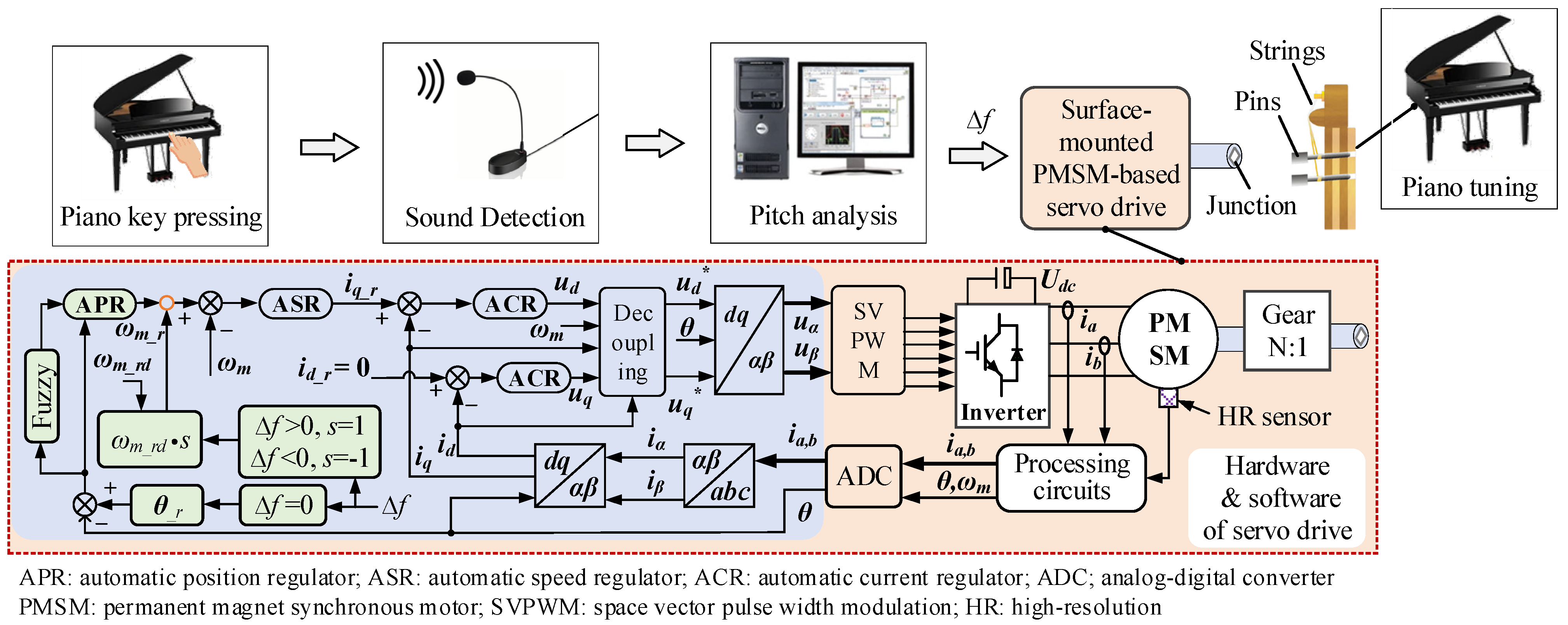
The structure of the proposed piano tuning devices is shown in Figure 1, which are mainly composed of a sound detection device, a pitch analysis device, surface-mounted permanent magnet synchronous motor-based actuators and the components of the piano. The sound detection device is a microphone, collecting the sounds generated by each string. The sound detection device is connected with a computer, on which a sound analysis software is installed, and they constitute the pitch analysis device. When the sound is input into the computer, the fundamental frequency of the signal (representing the tension of the string) can be extracted by using fast Fourier transform algorithms, which can be used to judge the intonation [8,31,32]. Then, the detected frequency is compared with the standard value, which is stored in the computer. It must be mentioned that the standard fundamental frequencies of all strings can be provided by the piano manufacturers, and the users can enter them into the analysis software manually. After pitch analysis, the error (∆f) between the detected frequency and the standard frequency is treated as the control signal of the surface-mounted permanent magnet synchronous motor-based drive, determining whether the double closed-loop speed-regulation algorithm or the triple closed-loop position-regulation algorithm should be used to control the electric motors. The motor shaft is connected with gears, reducing the output speed and increasing the output torque of the actuator. Finally, a junction at the end of the shaft of the output gear, which matches the head of the pins, can turn the pins so as to change the tension of the strings.

When using the proposed devices to tune a piano automatically, the implementation procedures are as follows (see Figure 2):

Step 1: The user plays one note, and the corresponding string generates sounds which are a mixture of sinusoidal tones at different fundamental frequencies.

Step 2: The sound detection device collects the sounds and transmits the signals into the pitch analysis device.

Step 3: The pitch analysis device extracts the fundamental frequencies of the sounds and compares them with the pre-input standard frequencies.

Step 4: The frequency errors ∆f are used to control the surface-mounted permanent magnet synchronous motor-based servo drive system. The goal of this step is as follows: If ∆f is not zero, turn the pins of the piano to reduce the errors. If ∆f reaches zero, the pins exactly maintain at the position. The logic of how to use ∆f to actuate the drive system will be detailed in Section 2.2.

Step 5: The tuning process is repeated until the pitch of the string is in tune, which can be represented by the frequency error displayed on the pitch analysis device.

2.2. Surface-Mounted Permanent Magnet Synchronous Motor-Based Servo Drive System

As shown in Figure 1, the servo drive system is composed of hardware and software of the surface-mounted permanent magnet synchronous motor drive, and gear. This part mainly illustrates them and the design methods with reference to the aforementioned functional requirements (low-speed rotation and position holding). In addition, considering that the surface-mounted permanent magnet synchronous motor drive is the core of the servo system, of which control parameters are required to be tuned in practice, the mathematical model of it is established, laying the ground for further analysis in Section 2 and Section 3.

a) Hardware

The hardware of the surface-mounted permanent magnet synchronous motor drive contains four main parts (see Figure 1), including a direct-current source that supplies power and voltage to the system, an inverter that converts direct current power into alternating current power, a motor that converts the electrical energy to the mechanical one, and the signal processing components (analog circuits and digital signal processor, etc.) As for the gear, it is part of the hardware of the servo system as well, connecting with the motor shaft (with gear ratio of N:1) and provides a junction to match with the pins of the piano. In order to satisfy the functions of low-speed rotation and position holding, the following points need to be noted at the design stage.

On the one hand, firstly, [12] illustrates that the maximum output rotating speed of the gear is 2.4°/s (0.042 rad/s). However, the literature also clarifies that although this speed can ensure a relatively high precision, it is still possible that large tuning errors can be generated. This represents in a lower pin-turning speed, which should be considered in an automated piano tuning system. Hence, as for a surface-mounted permanent magnet synchronous motor-based tuning device, which can operate stably in low-speed conditions, the operating speed can be designed as half of the maximum value, that is, 1.2°/s (0.021 rad/s). Secondly, in order to employ a gear with a moderate gear ratio, which is with high precision [33], the rated speed ω_{m_rd} of the surface-mounted permanent magnet synchronous motor can be designed as 2.1 rad/s (20 rpm), at which many surface-mounted permanent magnet synchronous motor servo motors can work stably without significant ripples. Thirdly, since the motor speed and the output speed of the tuning device are determined, the gear ratio r can be selected:

$$r=\frac{N}{1}=\frac{20}{0.2}=\frac{100}{1}$$

(1)

In practice, the gear box DKM 8GBK100BH is a good choice for speed reduction in the servo drive system.

On the other hand, to take full advantage of the position holding function of a surface-mounted permanent magnet synchronous motor drive, it is necessary to install a position sensor with high resolution in the motor. In this aspect, resolvers and encoders are competitive sensor alternatives [34]. However, compared with the encoders, considering that the resolvers have the advantages of high stability and high adaptability, it is more suitable for the piano tuning application. Practically, a resolver and a 16-bit resolution tracking resolver-to-digital (R/D) converter AD2S1210 can be used to constitute the system [25]. In this case, the resolution res (minimum position changing step in mechanical position) of the sensor can be calculated as:

$$res=\frac{{360}^{\circ }}{p_r(2^{16}-1)}$$

(2)

where p_r is the number of pole pairs of the resolver. Based on (2), it is obvious that when p_r = 1, res is 0.0055°. And if p_r rises, the minimum resolvable position will get smaller (higher resolution). It must be mentioned that because the rotor speed is calculated based on the position information, the resolver with high resolution contributes to lower speed detection ripples as well, helping to exert the aforementioned function of low-speed rotation.

b) Software

As shown in Figure 1, two different control schemes are incorporated, which are selected by the frequency error ∆f. Specifically, after ∆f is detected, the sign of its value is judged. When ∆f is non-zero, the double closed-loop speed-regulation scheme with good low-speed control performance [34] is adopted, and when ∆f is zero, the triple closed-loop position-regulation scheme with a marked position control performance [35] is adopted for control.

The implementations of the double closed-loop speed-regulation strategy are as follows:

Step 1: Speed reference calculation: If ∆f > 0, s₁ = 1, but if ∆f < 0, s₁ = −1. Then, the reference speed ω_{m_r} is calculated as:

$${\omega }_{m\_r}={\omega }_{m\_rd}{s}_1$$

(3)

Based on (3), when ∆f is positive, the motor rotates positively. Otherwise, it reverses. These show that the corresponding string of the piano is tightened or loosened, respectively.

Step 2: State measurement and coordinate transformation: The phase currents i_a, i_b, rotor position θ and rotating speed ω_m are measured by using sensors. Then, the currents are transformed to the direct-quadrature (d,q)-axis currents i_d, i_q by using i_a, i_b and θ [34], with intermediate variables (α,β-axis currents) i_α, i_β.

Step 3: Speed regulation and current reference generation: The error between ω_{m_r} and ω_m passes through an automatic speed regulator, generating q-axis current reference i_{q_r}. Then, considering that for a surface-mounted permanent magnet synchronous motor, the largest torque will be generated under the fixed current when the d-axis current remains at zero, the d-axis current reference i_{d_r} is set as 0 in this research (see Figure 1).

Step 4: Current regulation: The errors between i_{q_r} and i_q, and between i_{d_r} and i_d pass through two automatic current regulators, respectively.

Step 5: Space vector pulse width modulation signal generation: The outputs of the two automatic current regulators are adopted to generate control signals based on the space vector pulse width modulation theories [34].

Step 6: Actuation: The space vector pulse width modulation signals are applied to the inverter and motor.

The implementations of the triple closed-loop position-regulation strategy are as follows:

Step 1: Position reference determination: When the frequency error ∆f is zero, the instantaneous rotor position θ_{_r} is recorded, and it is set as the position reference. In this case, the rotor position is expected to be controlled to maintain at θ_{_r}.

Step 2: Position regulation and speed reference calculation: The error between θ_{_r} and θ passes through an automatic position regulator whose parameters need to be tuned using a fuzzy controller. The output of the automatic position regulator is treated as the speed reference ω_{m_r}.

Step 3~Step 7 are consistent with Step 2~Step 6 in the above implementation procedures of the double closed-loop speed-regulation scheme.

From the above analysis, the main difference between the two control techniques is that their control objectives are different. Besides, the purpose of the double closed-loop speed-regulation strategy is to adjust the pitch of the string to approaching the standard value, while the triple closed-loop position-regulation is able to eliminate the overshoot caused by the double closed-loop speed-regulation so as to achieve accurate tuning. Finally, it must be mentioned that in terms of the speed regulation and current regulation parts, they share the identical control algorithms.

c) Modeling of Surface-Mounted Permanent Magnet Synchronous Motor drive

The models of the main components (motor, inverter and proportional integral controller) of the surface-mounted drive, which are needed for parameter tuning in this paper, are established in this part.

Firstly, assuming that the iron saturation and hysteresis loss are assumed negligible [36], the mathematical model describing the electrical and mechanical dynamics of a surface-mounted permanent magnet synchronous motor in the d, q rotating frame is:

$$\frac{\mathrm{d}{i}_d}{\mathrm{d}t}=-\frac{R_s}{L_s}{i}_d+p{\omega }_m{i}_q+\frac{{u_d}^{*}}{L_s}$$

(4)

$$\frac{\mathrm{d}{i}_q}{\mathrm{d}t}=-p{\omega }_m{i}_d-\frac{R_s}{L_s}{i}_q+\frac{{u_q}^{*}}{L_s}-\frac{{\Psi }_f}{L_s}p{\omega }_m$$

(5)

$$\frac{\mathrm{d}{\omega }_m}{\mathrm{d}t}=\frac{1}{J}(\underset{T_e}{\underbrace{1.5p_m{\Psi }_f{i}_q}}-T_l-B{\omega }_m)$$

(6)

where u_d*, u_q* are the dq-axis control voltages without considering decoupling (see Figure 1). The stator winding resistance is R_s. Ψ_f is the rotor flux. L_s is the stator inductance of the motor. T_l is the load torque, and T_e is the electromagnetic torque. Then, p_m represents the number of pole pairs of the motor. J is the inertia of the rotor and B is the friction coefficient. From (4) and (5), it can be seen that a coupling effect exists, which will degrade the control performance. Therefore, in real applications, a feedback decoupling method is usually adopted to solve the problem, as shown in Figure 3.

After decoupling, the electrical model of the machine can be reconstructed as:

$$\frac{\mathrm{d}{i}_d}{\mathrm{d}t}=-\frac{R_s}{L_s}{i}_d+\frac{u_d}{L_s}$$

(7)

$$\frac{\mathrm{d}{i}_q}{\mathrm{d}t}=-\frac{R_s}{L_s}{i}_q+\frac{u_q}{L_s}$$

(8)

where u_d, u_q are the dq-axis control voltages with decoupling considered. Furthermore, applying the Laplace Transformation to (6)–(8), the motor model (taking the q-axis properties as an example) in the s-domain can be depicted in Figure 4, where T_l can be regarded as an external disturbance.

Secondly, ignoring the delay effects of the dead zone and switch delay, the inverter can be described by a first-order model:

$$G_{inv}(s)=\frac{k_{inv}}{s·T_s+1}$$

(9)

where k_inv is the magnification of the inverter, and it is 1 when the space vector pulse width modulation strategy is adopted. T_s is the switching period.

Thirdly, as for the automatic speed regulator, automatic current regulators and automatic position regulator (proportional integral controllers), the transfer functions of them are:

$$G_{ASR}(s)=k_{s\_p}+\frac{k_{s\_i}}{s},G_{ACR}(s)=k_{c\_p}+\frac{k_{c\_i}}{s},G_{APR}(s)=k_{p\_p}+\frac{k_{p\_i}}{s}$$

(10)

where k_{s_p}, k_{c_p} and k_{p_p} are the scaling factors, and k_{s_i}, k_{c_i} and k_{p_i} are the scaling and integral factors of the automatic speed regulator, automatic current regulators and automatic position regulator, respectively.

3. Proportional Integral Controller Design for Double Closed-Loop Speed-Regulation Scheme

As shown in Figure 1, one automatic speed regulator and two automatic current regulators are incorporated into the double closed-loop speed-regulation control scheme. The parameters of them are closely related to the speed performance. Specifically, if parameters of the controllers endow the surface-mounted permanent magnet synchronous motor drive with a large bandwidth, although the system response speed is high, the external disturbances are more inclined to bring about speed ripples. Undoubtedly, this reduces the accuracy of the pin-turning process. However, as illustrated in Section 2, when the motor needs to rotate, its speed should stabilize at a constant value. In this case, a fast response is unnecessary, leading to the fact that a large bandwidth is not required. Instead, to increase speed stability and piano-tuning accuracy, the parameters of the proportional integral controllers are supposed to be tuned, endowing the system with a low bandwidth. Overall, this part introduces a parameter tuning design method based on amplitude-frequency analysis, which includes two sequential stages: (1) current-loop analysis, and (2) speed-loop analysis.

3.1. Current-Loop Analysis

Considering that the parameters of the d-axis and q-axis automatic current regulators can be set as the same values for the surface-mounted permanent magnet synchronous motor drives in practice, as long as the parameters of the q-axis controller are tuned, the parameters of the d-axis one can be determined simultaneously. For the sake of intuitiveness, the control diagram of the q-axis current loop is illustrated in Figure 5. The open-loop transfer function G_ot(s) and the closed-loop transfer function G_ct(s) can be described as in (11) and (12), respectively. When designing the proportional integral controllers used in the piano-tuning applications, the main tasks include: stability analysis and bandwidth analysis, which can only rely on the closed-loop transfer function.

$$G_{ot}(s)=G_{ACR}(s)·G_{inv}(s)·G_e(s)=\frac{k_{c\_p}s+k_{c\_i}}{L_s{T}_s{s}^3+(R_s{T}_s+L_s)s^2+R_{s}s}$$

(11)

$$G_{ct}(s)=\frac{G_{ot}(s)}{1+G_{ot}(s)}=\frac{k_{c\_p}s+k_{c\_i}}{L_s{T}_s{s}^3+(R_s{T}_s+L_s)s^2+(R_s+k_{c\_p})s+k_{c\_i}}$$

(12)

a) Stability analysis

Based on (12), the characteristic equation D_c(s) of the system can be written as:

$$D_c(s)=L_s{T}_s{s}^3+(R_s{T}_s+L_s)s^2+(R_s+k_{c\_p})s+k_{c\_i}$$

(13)

Then, in order to use the Routh’s stability criterion to analyze the stability of the system,

Table 2. Routh table of current control loop.

s3	Ls·Ts	Rs + kc_p
s2	RsTs + Ls	kc_i
s1	$\frac{(R_s{T}_s+L_s)(R_s+k_{c\_p})-L_s{T}_s{k}_{c\_i}}{R_s{T}_s+L_s}$	0
s0	kc_i	0

shows the Routh table of the current control loop. To make the current control loop stable, the following equations require must be satisfied:

$$\{\begin{array}{l}{L}_s{T}_s>0\\ R_s{T}_s+L_q>0\\ \frac{(R_s{T}_s+Ls)(R_s+k_{c\_p})-L_s{T}_s{k}_{c\_i}}{R_s{T}_s+L_s}>0\\ k_{c\_i}>0\end{array}\to \{\begin{array}{l}{k}_{c\_p}>\frac{L_s{T}_s{k}_{c\_i}}{R_s{T}_s+L_s}-R_s\\ k_{c\_i}>0\end{array}$$

(14)

Obviously, from the current control loop, it can be seen that the system stability is related to the parameters of the drive system, such as the machine inductance, resistance and sampling period. What can be directly derived from (14) is that, firstly, the integral factor of the automatic current regulator should be positive, and secondly, that it is more complicated to illustrate the range of the scaling factor. For the sake of intuitiveness, a surface-mounted permanent magnet synchronous motor whose parameters are given in

Table 3. Parameters of Surface-Mounted Permanent Magnet Synchronous Motor.

Parameters	Value	Unit
Stator inductance Ls	3	mH
Stator resistance Rs	0.08	Ω
Number of motor pole pairs pm	3	-
Number of resolver pole pairs pr	3	-
inertia of the rotor J	0.0003	kg·m2
Direct-current-bus voltage Udc	48	V
Rated speed ωm_rd	2.1	rad/s

is taken as an example to present the relationship of the scaling factor versus k_{c_i} and T_s (see Figure 6). In Figure 6, to make the system stable, k_{c_p} should be over the critical plane and k_{c_i} must be larger than zero. Besides, it can be noted that, on the one hand, when the integral factor (or the switching period) is fixed, the larger the switching period (or the integral factor) is, the larger k_{c_p} should be. On the other hand, the range of k_{c_p} is large. In other words, k_{c_p} can be set as a very small value, where even k_{c_i} stands at a relatively high position.

b) Bandwidth analysis

The bandwidth of a system can be reflected by the amplitude-frequency characteristics. Based on the automatic control theories, the bandwidth of the system is defined as the frequency range between zero and the upper limit at which the magnification decreases to 70.7% of the magnitude when the frequency is zero [37]. Theoretically, the smaller the bandwidth is, the stronger the anti-interference capacity of a system becomes. On the contrary, if a system has a large bandwidth, although the response speed grows, the disturbances are more inclined to be introduced. To ensure a high piano-tuning accuracy, the bandwidth of the system needs to be limited.

As for (12), the amplitude-frequency characteristic can be obtained as follows:

$$G_{ct}(j\omega )=\frac{k_{c\_p}j\omega +k_{c\_i}}{-L_s{T}_{s}j{\omega }^3-(R_s{T}_s+L_s){\omega }^2+(R_s+k_{c\_p})j\omega +k_{c\_i}}$$

(15)

Then, the magnitude of G_ct when ω = 0 can be calculated as:

$$M_c(0)=|G_{ct}(j\omega ){|}_{\omega =0}=1$$

(16)

where M_c(0) represents the magnitude of G_ct when ω = 0. Hence, based on the definition of the bandwidth, the bandwidth of the current loop can be obtained by solving the following equation:

$$\begin{array}{l}{|G_{ct}(j\omega )|}_{\omega ={\omega }_{b\_c}}=0.707M_c(0)\\ \to |\frac{k_{c\_p}j{\omega }_{b\_c}+k_{c\_i}}{-L_s{T}_{s}j{{\omega }_{b\_c}}^3-(R_s{T}_s+L_s){{\omega }_{b\_c}}^2+(R_s+k_{c\_p})j{\omega }_{b\_c}+k_{c\_i}}|=0.707\end{array}$$

(17)

where ω_{b_c} is the bandwidth of the current loop. Unluckily, there are no specific solutions (ω_{b_c}) to (17). Hence, the formula needs to be simplified properly. As for a servo permanent magnet synchronous motor whose parameters are similar to those in Table 3, the orders of magnitude (OD) of L_s, T_s and R_s are 0.001, 0.0001, 0.1, respectively. Hence, the following conditions are satisfied:

$$\underset{\mathrm{OD}={10}^{-7}}{\underbrace{L_s{T}_s}}<<\underset{\mathrm{OD}={10}^{-3}}{\underbrace{R_s{T}_s+L_s}}<<\underset{\mathrm{OD}>0.1}{\underbrace{R_s+k_{c\_p}}}$$

(18)

Ignoring the impacts of the small terms, (17) can be simplified as:

$$|\frac{k_{c\_p}j{\omega }_{b\_c}+k_{c\_i}}{(R_s+k_{c\_p})j{\omega }_{b\_c}+k_{c\_i}}|\approx 0.707$$

(19)

And ω_{b_c} can be calculated as:

$${\omega }_{b\_c}=\frac{k_{c\_i}}{\sqrt{4R_s{k}_{c\_p}-2{R_s}^2}}$$

(20)

In addition, as for the surface-mounted permanent magnet synchronous motor working at the rated speed ω_{m_rd} during the piano-tuning process, the frequency of the phase currents ω_current are:

$${\omega }_{current}=p_m{\omega }_{m\_rd}$$

(21)

In practice, ω_{b_c} should be designed to be larger than ω_current, and only by this can the motor work normally during control; that is,

$${\omega }_{b\_c}=\frac{k_{c\_i}}{\sqrt{4R_s{k}_{c\_p}-2R_s{}^2}}>p_m{\omega }_{m\_rd}$$

(22)

Considering that the speed of the servo motor is low, even ω_{b_c} is set as ten times of ω_current, the overall bandwidth of the system is not large, and this is adopted in this research. Hence, it can be derived that:

$$k_{c\_i}=10p_m{\omega }_{m\_rd}\sqrt{4R_s{k}_{c\_p}-2{R_s}^2}$$

(23)

Further, combining (14) and (23), the automatic current regulator parameters that can ensure both stability and low bandwidth can be obtained as:

$$\{\begin{array}{l}{k}_{c\_p}>\max (\frac{L_s{T}_s{k}_{c\_i}}{R_s{T}_s+L_s}-R_s,0.5R_s)\\ k_{c\_i}=10p_m{\omega }_{m\_rd}\sqrt{4R_s{k}_{c\_p}-2{R_s}^2}\end{array}$$

(24)

When using (24) to design the automatic current regulator, firstly, k_{c_p} is set as a value that is larger than 0.5R_s. Then, substitute the selected k_{c_p} into the second equation in (24) to calculate k_{c_i}. Finally, use the first inequation in (24) to judge whether the values of k_{c_p} and k_{c_i} are suitable. For example, for the surface-mounted permanent magnet synchronous motor drive whose parameters are consistent with those in Table 3 (when the switching period T_s = 0.1 ms), the parameters of the automatic current regulator can be designed as k_{c_p} = 0.5 and k_{c_i} = 24 for a case study in this paper.

3.2. Speed-Loop Analysis

Since the current control loop has been analyzed, its transfer function G_ct(s) can be directly incorporated into the control diagram of the speed loop used for automatic speed regulator design (see Figure 7). To analyze the stability and bandwidth characteristics, with reference to (12), treat the load torque as the external disturbance and the speed-loop transfer function of the system G_{ct_sp}(s), which can be written as:

$$\{\begin{array}{l}{G}_{ct\_sp}(s)=\frac{1.5p{\Psi }_f[k_{s\_p}{k}_{c\_p}{s}^2+(k_{s\_p}{k}_{c\_i}+k_{s\_i}{k}_{c\_p})s+k_{s\_i}{k}_{c\_i}]}{a_4{s}^4+a_3{s}^3+a_2{s}^2+a_{1}s+a_0}\\ a_4=J{L}_s{T}_s·\\ a_3=J{R}_s{T}_s+J{L}_s+B{L}_{s}T\\ a_2=J{R}_s+J{k}_{c\_p}+B{R}_s{T}_s+B{L}_s+1.5p{\Psi }_f{k}_{s\_p}{k}_{c\_p}\\ a_1=J{k}_{c\_i}+B{R}_s+B{k}_{c\_p}+1.5p{\Psi }_f{k}_{s\_p}{k}_{c\_i}+1.5p{\Psi }_f{k}_{s\_i}{k}_{c\_p}\\ a_0=B{k}_{c\_i}+1.5p{\Psi }_f{k}_{s\_i}{k}_{c\_i}\end{array}$$

(25)

a) Stability analysis

Based on (25), the characteristic equation D_sp(s) of the system can be written as:

$$D_{sp}(s)=a_4{s}^4+a_3{s}^3+a_2{s}^2+a_{1}s+a_0$$

(26)

The Routh table of the speed loop is shown in

Table 4. Routh table of speed loop.

s4	a4	a2	a0
s3	a3	a1	0
s2	$\frac{a_2·a_3-a_1·a_4}{a_3}$	a0	0
s1	$\frac{a_1·a_2·a_3-{a_1}^2·a_4-a_0·{a_3}^2}{a_2·a_3-a_1·a_4}$	0	0
s0	a0	0	0

. To make the system stable, the following equations must be satisfied:

$$\{\begin{array}{l}{a}_4>0\\ a_3>0\\ \frac{a_2{a}_3-a_1{a}_4}{a_3}>0\\ \frac{a_1{a}_2{a}_3-a_1{}^2{a}_4-a_0{a}_3{}^2}{a_2{a}_3-a_1{a}_4}>0\\ a_0>0\end{array}\to \{\begin{array}{l}\frac{a_2{a}_3-a_1{a}_4}{a_3}>0\\ \frac{a_1{a}_2{a}_3-{a_1}^2{a}_4-a_0{a_3}^2}{a_2{a}_3-a_1{a}_4}>0\\ a_0>0\end{array}$$

(27)

Being different to (14), after substituting (25) into (27), even though k_{c_p} and k_{c_i} are known, the relation of k_{s_p}, k_{s_i} and the motor parameters are still complicated, which cannot be described using intuitive expressions. Hence, instead of directly illustrating the inherent properties reflected by (27), the method of how to use it to design the parameters of the automatic speed regulator will be synthesized after bandwidth analysis.

b) Bandwidth design

Unlike the current loop, whose bandwidth mainly influences the current performance, the bandwidth of the speed loop is closely related to the disturbances introduced by the speed. Considering that the speed can be regarded as a constant value (zero frequency) when the machine operates stably, the speed-loop bandwidth can be designed to be very low theoretically [38], which contributes to attenuating the speed ripples caused by the external disturbances.

Substituting jω into (25), the amplitude-frequency characteristic can be obtained:

$$G_{ct\_sp}(j\omega )=\frac{1.5p{\Psi }_f[-k_{s\_p}{k}_{c\_p}{\omega }^2+(k_{s\_p}{k}_{c\_i}+k_{s\_i}{k}_{c\_p})j\omega +k_{s\_i}{k}_{c\_i}]}{a_4{\omega }^4-a_{3}j{\omega }^3-a_2{\omega }^2+a_{1}j\omega +a_0}$$

(28)

And the magnitude M_sp(0) of G_{ct_sp} when ω = 0 is:

$$M_{sp}(0)=|G_{ct}(j\omega ){|}_{\omega =0}=\frac{1.5p{\Psi }_f{k}_{s\_i}{k}_{c\_i}}{B{k}_{c\_i}+1.5p{\Psi }_f{k}_{s\_i}{k}_{c\_i}}$$

(29)

Hence, the bandwidth of the speed loop can be obtained by solving the following equation:

$$\begin{array}{l}{|G_{ct\_sp}(j\omega )|}_{\omega ={\omega }_{b\_sp}}=0.707M_{sp}(0)\\ \to |\frac{-k_{s\_p}{k}_{c\_p}{\omega }_{b\_sp}{}^2+(k_{s\_p}{k}_{c\_i}+k_{s\_i}{k}_{c\_p})j{\omega }_{b\_sp}+k_{s\_i}{k}_{c\_i}}{a_4{\omega }_{b\_sp}{}^4-a_{3}j{\omega }_{b\_sp}{}^3-a_2{\omega }_{b\_sp}{}^2+a_{1}j{\omega }_{b\_sp}+a_0}|=\frac{0.707k_{s\_i}{k}_{c\_i}}{B{k}_{c\_i}+1.5p{\Psi }_f{k}_{s\_i}{k}_{c\_i}}\end{array}$$

(30)

where ω_{b_sp} is the bandwidth of the speed loop. Similarly, there are no analytical solutions (ω_{b_sp}) to (30) because it is an eight-order equation. In this case, even using the simplification method that ignores the terms with low ODs, it is not easy to solve (30) either, and the reasons are as follows. By analyzing the ODs of a₀, a₁, a₂, a₃ and a₄, a₃ and a₄ are small enough to be ignored compared to a₀, a₁ and a₂. This happens because the latter three variables contain 1.5pΨ_fk_{s_p}k_{c_p}, 1.5pΨ_fk_{s_i}k_{c_p} and 1.5pΨ_fk_{s_i}k_{c_i}, respectively, in which p, Ψ_f and the controller parameters are usually much larger than the parameters (including inductance, resistance and switching period, etc.) of the surface-mounted permanent magnet synchronous motor drive. However, when a₃ and a₄ are set as zero, (30) becomes a four-order equation, which is still a difficult mathematical problem. On this ground this part employs a “direct bandwidth setting” method to design k_{s_p} and k_{s_i}. In detail, according to [38], there is no lower limit for the bandwidth of the speed loop because the working frequency of this loop is nearly zero in theory. In this research, for a low-speed servo drive, ω_{b_sp} is selected as twice the magnitude of the rated speed; that is,

$${\omega }_{b\_sp}=2{\omega }_{m\_rd}$$

(31)

Furthermore, substitute (31) into (30) and the relationship between k_{s_p} and k_{s_i} can be derived as:

$$\{\begin{array}{l}\frac{\sqrt{{(k_{s\_i}{k}_{c\_i}-4k_{s\_p}{k}_{c\_p}{\omega }_{m\_rd}{}^2)}^2+4{(k_{s\_p}{k}_{c\_i}+k_{s\_i}{k}_{c\_p})}^2{\omega }_{m\_rd}{}^2}}{\sqrt{{(a_5-6p{\Psi }_f{k}_{s\_p}{k}_{c\_p}{\omega }_{m\_rd}{}^2+1.5p{\Psi }_f{k}_{s\_i}{k}_{c\_i})}^2+{(a_6+3p{\Psi }_f{k}_{s\_p}{k}_{c\_i}{\omega }_{m\_rd}+3p{\Psi }_f{k}_{s\_i}{k}_{c\_p}{\omega }_{m\_rd})}^2}}=\frac{0.707k_{s\_i}{k}_{c\_i}}{B{k}_{c\_i}+1.5p{\Psi }_f{k}_{s\_i}{k}_{c\_i}}\\ \\ a_5=16a_4{\omega }_{m\_rd}{}^4-4(J{R}_s+J{k}_{c\_p}+B{R}_s{T}_s+B{L}_s){\omega }_{m\_rd}{}^2+B·k_{c\_i}\\ a_6=2(J·k_{c\_i}+B·R_s+B·k_{c\_p}){\omega }_{m\_rd}-8a_3{\omega }_{m\_rd}{}^3\end{array}$$

(32)

So far, (27) and (32) constitute the parameter design criteria for automatic speed regulators. When using them, firstly, set k_{s_p} as a positive value artificially. Then, substitute it into (32) to calculate k_{s_i}. It must be mentioned that the designed k_{s_p} and k_{s_i}, which satisfy (32), can ensure that the speed loop has a low bandwidth. Finally, substitute k_{s_p} and k_{s_i} into (27) to judge if they can make the system stable. Finally, as for the surface-mounted permanent magnet synchronous motor drive shown in Table 3, for a case study, if T_s = 0.1 ms, k_{c_p} = 0.5 and k_{c_i} = 24, the automatic speed regulator parameters can be set as k_{s_p} = 1 and k_{s_i} = 32.35.

4. Fuzzy-Adaptive Proportional Integral Controller Design for Triple Closed-Loop Position-Regulation Scheme

As illustrated in Section 2.2, the automatic position regulator is employed to control the surface-mounted permanent magnet synchronous motor rotor to accurately maintain the position where ∆f makes zero. The position control loop is able to eliminate the overshoot caused by the double closed-loop speed-regulation strategy effectively, avoiding slight deviations. The position control process can be divided into two stages: overshoot elimination and position holding. Comparatively speaking, the former stage requires a relatively higher response speed, while the latter one needs a stronger anti-interference capability. Hence, it is necessary to design an adaptive bandwidth to achieve the goals. This section introduces a fuzzy adaptive proportional integral controller with a higher bandwidth in the overshoot elimination stage, and with a lower bandwidth in the position-holding stage.

4.1. Proposed Fuzzy Afdaptive Proportional Integral Controller

The detailed block diagram of the proposed fuzzy adaptive proportional integral controller (see Figure 2) is depicted in Figure 8, where ∆θ is the error between the reference position and the real position, K_in is the input scaling factor. In, Out_p and Out_i are the input and outputs of the fuzzy inference engine, respectively, D_p and D_i are the outputs of the defuzzification component, K_op and K_oi are the output scaling factors, Δk_{p_p} and Δk_{p_i} are the compensation values for automatic position regulator parameters, k_{p_p0} and k_{p_i0} are the initial scaling and integral factors for the automatic position regulator, k_{p_p} and k_{p_i} are the real scaling and integral factors, ω_{m_r} is the output of the automatic position regulator and it represents the reference speed.

As for the proposed fuzzy adaptive controller, there are three main features which need to be addressed. Firstly, the fuzzy controller is a single-input-two-output controller. This is not a typical two-dimensional controller that uses both the error of control variable (position) and the differential of the error as the inputs [39]. This structure is reasonable because in the piano tuning applications, the change rate of ∆θ is small enough to be detected when the position loop works. Hence, as long as an overshoot can be distinguished, suitable proportional integral parameters can be generated. Secondly, the operating mechanisms of the fuzzy adaptive proportional integral controller can be described as being if ∆θ is small, or even zero, the fuzzy controller will generate compensations that endow the system with a small bandwidth, but if ∆θ is large, the proportional integral controller parameters used for control should ensure a relatively large bandwidth. Thirdly, the fuzzy controller contains five parts, namely, fuzzification, fuzzy control rules, membership function, defuzzification and adjustment, and their design processes will be detailed next.

4.2. Design of Fuzzy Controller

4.2.1. Fuzzification

By using the fuzzification component, the inputs are converted to the values in the fuzzy domain. Based on the standardization control theory, the fuzzy domain can be set as [−1, 1] [40]. Therefore, K_in can be set as the reciprocal of the maximum position error ∆θ_max, namely,

$$K_{in}=\frac{1}{\Delta {\theta }_{\max }}$$

(33)

It should be noted that ∆θ_max is not a certain value, and instead, it is an anticipated value. In other words, the designer can artificially determine the magnitude of it. In this research, that the position overshoot reaches 0.5° (0.0087 rad) is treated as the worst condition, thereby ∆θ_max = 0.0087.

4.2.2. Fuzzy Control Rules

The fuzzy control rules are adopted to build bridges between the input and the outputs. In order to create appropriate control rules, linguistic expressions are supposed to be defined. In this research, the linguist expressions are positive large (PL), positive medium (PM), positive small (PS), zero (ZO), negative small (NS), negative medium (NM) and negative large (NL). For the output Out_p corresponding to the proportional integral scaling factor, the fuzzy subset is {ZO, NS, NM, NL}, while for Out_i corresponding to the integral factor, the subset is {ZO, PS, PM, PL}. The rationale behind these settings is that the initial parameters k_{p_p0} and k_{p_i0} are designed to endow the system with a pretty large bandwidth, which will be detailed in Section 4.2.4. As for the variable In, the fuzzy subset is {PL, PM, PS, ZO, NS, NM, NL} because it can be either negative or positive.

Table 5. Fuzzy control rules for scaling factor.

In	PL	PM	PS	ZO	NS	NM	NL
Outp	ZO	NS	NM	NL	NM	NS	ZO

and

Table 6. Fuzzy control rules for integral factor.

In	PL	PM	PS	ZO	NS	NM	NL
Outi	ZO	PS	PM	PL	PM	PS	ZO

present the fuzzy control rules extracted from the existing knowledge for the scaling and integral parameters, respectively, which can be summarized as follows: the larger the magnitude of Δθ is, the smaller the compensation values (∆k_{p_p},∆k_{p_i}) for automatic position regulator parameters are.

Relying on Table 5 and Table 6, the fuzzy control rules can be defined as the form of “if-then”, that is,

If In is A, Then Out_p is B and Out_i is C.

where A is the fuzzy subset corresponding to the input In. B and C are the fuzzy subsets corresponding to the outputs Out_p and Out_i, respectively.

4.2.3. Membership Functions

For a fuzzy controller, the membership functions represent the degree of truth, working together with the control rules to solve the fuzzy inference problem quantitatively. The membership functions for In, Out_p and Out_i are depicted in Figure 9. It can be seen that in Figure 9a, the outputs of the function are between 0 and 1, while the inputs range from −1 to 1. In Figure 9b,c, although the degree of membership is still between 0 and 1, the fuzzy domain becomes [−1, 0] and [0, 1], respectively, which are consistent with the corresponding fuzzy subsets. Besides, it can be seen that intersections of NM and NL domains in Figure 9b and intersections of PM and PL domains in Figure 9c are weak. This draws clear lines between the large range and medium range for the output compensation values. In the piano tuning process, this kind of membership function is sensitive once the position error is small, reducing the system bandwidth efficiently.

4.2.4. Defuzzification

Because Out_p and Out_i are still fuzzy sets, they cannot be directly adopted for adjusting the parameters of the automatic position regulator. Therefore, they must be converted to explicit values by using a defuzzification component. In engineering, the most commonly-used strategy is the centroid defuzzification which contains most of the inference results [39]:

$$\{\begin{array}{l}{D}_p=\frac{{\displaystyle \sum _{i=1}^m{x}_i·v(x_i)}}{{\displaystyle \sum _{i=1}^{m}v(x_i)}}\\ D_i=\frac{{\displaystyle \sum _{i=1}^m{y}_i·u(y_i)}}{{\displaystyle \sum _{i=1}^{m}u(y_i)}}\end{array}$$

(34)

where m is the number of membership functions, v(x_i) and u(y_i) are the membership degrees corresponding to the output scaling and integral factor compensations, x_i and y_i are the values corresponding to their membership degrees.

4.2.5. Adjustment

After defuzzification, the ranges of the outputs D_p and D_i are [−1, 0] and [0, 1], respectively. Then, the positive output scaling factors K_op and K_oi are required to adjust D_p and D_i to the decent values. Specifically, the compensation values ∆k_{p_p} and ∆k_{p_i} can be obtained by:

$$\{\begin{array}{l}\Delta k_{p\_p}=K_{op}·D_p\\ \Delta k_{p\_}{}_i=K_{oi}·D_i\end{array}$$

(35)

Finally, the real-time scaling and integral factors of the automatic position regulator can be described as:

$$\{\begin{array}{l}{k}_{p\_p}=k_{p\_p0}+\Delta k_{p\_p}\\ k_{p\_}{}_i=k_{p\_i0}+\Delta k_{p\_}{}_i\end{array}$$

(36)

where k_{p_p0} and k_{p_i0} are the initial scaling and integral factors, respectively, and as mentioned in Section 4.2.2, they should be specially designed. In detail, considering that a proportional integral controller will more or less reduce the bandwidth of the system inevitably on the basis of its properties [37], k_{p_p0} and k_{p_i0} can be set as values that rarely reduce the overall system bandwidth or the bandwidth of the double closed-loop speed-regulation structure. In this case, the following inequation needs to be satisfied:

$$k_{p\_p0}>>k_{p\_i0}$$

(37)

In this research, k_{p_p0} is ten times of k_{p_i0}. For example, k_{p_p0} = 3.5 and k_{p_i0} = 0.35 as a case study. Then, based on the existing knowledge, if the bandwidth of the system needs to be reduced, what we need to do is only to decrease the scaling factor and increase integral factor. This is the reason why the fuzzy subsets and membership functions for Out_p and Out_i are designed that way in Section 4.2.2 and Section 4.2.3.

5. Simulation Verifications

Considering that the main purpose of this paper is to develop a servo drive system for the automated piano tuning devices, simulation is conducted on a three-phase surface-mounted permanent magnet synchronous motor drive whose parameters are consistent with those in Table 3 to verify the effectiveness of the proposed surface-mounted permanent magnet synchronous motor-based servo drive system and validate the proposed control methods. Besides, the switching period of the system is set as 0.1 ms, and the parameters of the controllers comply with the typical values mentioned in the previous sections (as a case study), that is, k_{c_p} = 0.5 and k_{c_i} = 24, k_{s_p} = 1, k_{s_i} = 32.35, k_{p_p0} = 3.5 k_{p_i0} = 0.35. The simulation systems are shown in Figure 10, which are established in MATLAB/Simulink 2018a. The system in Figure 10a is mainly used for analyzing the performance of the proposed drive system (including structure and design methods), while the system in Figure 10b is used to simulate the real tuning process, with frequency response and frequency feedback considered (more complying with the realistic situations). As for the simulation concerning the performance of the drive system, what needs to be explained include that, firstly, the error (∆f) between the detected frequency and standard frequency of a piano string is given manually, simulating the sound detection device and pitch analysis device processes. Secondly, the desired output load torque of the motor is assumed to be 3 Nm, which can be further amplified through the gear. Thirdly, external disturbances are considered for the speed control and position control processes, which is going to prove that the controller parameter design methods based on bandwidth analysis have strong anti-interference capability. Fourthly, for the sake of comprehensiveness, four cases are analyzed in simulation: Case 1: ∆f is larger than zero; Case 2: ∆f is less than zero; Case 3: ∆f equals zero; Case 4: ∆f switches to zero from a nonzero value. In terms of the simulation considering realistic situations, one more case is analyzed: Case 5: the frequency adjustment characteristics are presented.

5.1. Case 1

That ∆f is larger than zero means that the motor needs to rotate positively. In this case, s₁ of the “control logic part” in Figure 11 is 1, s₂ is 1. Then, the double closed-loop speed-regulation control strategy will be used to actuate the motor. Between 0 and 5.0 s, the motor speed is directly fed back, while between 5.0 s and 10.0 s, white noises (magnitude is 1.0 rpm) are added to the feedback speed, simulating the external disturbances. Figure 11 shows the simulation setup and the control performance of the surface-mounted permanent magnet synchronous motor-based servo drive system when ∆f is larger than zero. Firstly, the machine speed can stabilize at the reference level and the currents are stable during the whole test. Secondly, when there are no external disturbances, the rotor speed ripples are about ± 0.5 rpm (0.052 rad/s). When the speed loop experiences external disturbances, the speed ripples increase slightly, which increases to ± 0.65 rpm (0.068 rad/s). The reason why the speed ripples become larger is that the white noises (disturbances) contain the low-frequency components, which can be introduced into the system inevitably. Finally, when the speed transfers to the gear, the output of it is stable as well. The maximum speed ripples arising from the motor side are ± 0.025 rpm and ± 0.0325 rpm in the first and the second half test period, respectively. This can ensure that the pins of the piano can be turned slowly, improving the accuracy of the piano tuning process.

5.2. Case 2

When ∆f < 0, the motor needs to rotate negatively. Hence, s₁ is −1 and s₂ is 1. The simulation setups are the same as those in Case 1. Figure 12 illustrates the simulation setup and the control performance of the surface-mounted permanent magnet synchronous motor-based servo drive system when ∆f is less than zero. It can be seen that, firstly, being similar to Figure 11, the speed and current are stable. Secondly, although the speed ripples between 5.0 s and 10.0 s are the same as those in Figure 11, between 0 and 10 s, they become ten percent higher. But it needs to be mentioned that the speed ripples still stand at low positions, which do not influence the accuracy of the piano tuning process.

By looking at the verification results of Case 1 and Case 2, it can be found that the surface-mounted permanent magnet synchronous motor-based servo drive can work stably over the low-speed conditions, which comply with the working environment of the piano tuning process. Hence, it can be concluded that a surface-mounted permanent magnet synchronous motor-based servo drive is applicable in practice.

5.3. Case 3

When ∆f = 0, the motor needs to rotate negatively. Hence, s₂ is −1. In this case, the triple closed-loop position-regulation control scheme is employed for motor control. For the sake of analysis, the rotor position is controlled to maintain at 1 rad in this part (θ_{_r} = 1). Between 0 and 5.0 s, the rotor position is directly fed back, while between 5.0 s and 10.0 s, the white noises (magnitude is 0.05 rad) are added to the feedback position, simulating the external disturbances. The simulation results when ∆f equals zero are demonstrated in Figure 13. It can be seen that the position can maintain at the references level with slight ripples. The ripples are ± 0.02 rad and ± 0.024 rad in the first and second half test period, respectively. This proves that the surface-mounted permanent magnet synchronous motor-based servo drive is able to exert a good position-holding function, achieving a high tuning accuracy.

5.4. Case 4

Figure 14 shows the performance of the servo drive system when ∆f switches to zero from 1.0 at 5.0 s. Firstly, between 0 and 5.0 s, the motor rotates stably and the rotor position continues to increase, and after about 7.5 s, the speed decreases to zero and the position levels off constantly. This illustrates that the proposed surface-mounted permanent magnet synchronous motor-based servo drive is able to achieve the low-speed rotation and position holding functions in the dynamic process. Secondly, At 5.0 s when ∆f changes, it takes a while before the rotor speed decreases to the same as those down to zero. In this period, the motor position must continue to increase, leading to position overshoot. This is inevitable for the proposed system, even if the fuzzy controller is adopted, because this is determined by the properties of the system. It must be mentioned that even for a direct-current motor-based or step motor-based servo drive system, when the pitch of a string is detected to be in tune, the bus voltage is removed to stop the tuning devices. The position overshoot is still inevitable because it must take a short time before the voltage and currents in the machine disappear totally. From the perspective of this point, the proposed surface-mounted permanent magnet synchronous motor drive with a high-resolution position sensor installed and position control algorithms integrated must have a higher tuning accuracy. Finally, at 5.0 s, the recorded rotor position is 31.235 rad. After 5.0 s, although the position overshoot occurs, the motor can rotate back and level off at 31.235 rad eventually. This represents that the proposed piano tuning strategy is of high precision.

5.5. Case 5

To verify the frequency characteristics in the process of the tuning, as is shown in Figure 10b, the standard frequency f_{_r} of the string is assumed to be 3.1 Hz. Besides, assume that the detected frequency f is positively related to the rotor position θ, which can be described as: f = 0.5θ. In the beginning, the rotor position is zero, and the frequency of the string is zero as well. In this case, ∆f is 3.1. Hence, the anticipated system performance characteristics are as follows. The motor speeds up to 20 rpm at first. When the rotor position reaches 6.2 rad, the position holding algorithm maintains the position at this level and maintains the motor speed at zero. In this process, the frequency error continuously declines. Figure 15 shows the simulation results of the tuning process. Between 0 and 2.98 s, and the frequency error approaches zero from 3.1 Hz. This happens because the motor speed is 20 rpm, adjusting the frequency to the standard value. An interesting phenomenon is that the dynamic speed, position and current performance characteristics are similar to those in Figure 14. This illustrates that no matter how the frequency error changes (modest or sharp change), the position and speed responses are similar when the frequency reaches the standard value. Especially, the speed will change from 20 or −20 to 0 immediately.

6. Conclusions

In order to simplify and improve the accuracy of the piano tuning process, this paper proposes an automated surface-mounted permanent magnet synchronous motor servo drive-based tuning technique. The main contributions of this paper include:

(1) The structure and principles of the automated surface-mounted permanent magnet synchronous motor servo drive-based tuning system are explained. The advantages of this kind of system over the direct-current/step motor-based system are that, firstly, the surface-mounted permanent magnet synchronous motor drive has higher control performance in the low-speed conditions, and secondly, the high-resolution position sensors are adopted to accurately achieve the position holding function.

(2) To ensure that the motor can work stably in the low-speed conditions, without being influenced by the external disturbances, both stability and bandwidth analyses are adopted to design the parameters of the automatic current regulator and automatic speed regulator. In this paper, the parameter design criteria that are suitable for the piano tuning applications are derived, which have seldom been studied previously.

(3) A fuzzy-adaptive proportional integral controller (structure, fuzzification, membership functions, fuzzy rules, deffuzification and adjustment) is specially designed to adapt to the piano tuning applications. Finally, simulation results prove that the proposed automated piano tuning techniques are effective.

References

1. Michon, R.; Smith, J.O.; Wright, M.; Chafe, C.; Granzow, J.; Wang, G. Mobile Music, Sensors, Physical Modeling, and Digital Fabrication: Articulating the Augmented Mobile Instrument. Appl. Sci. 2017, 7, 1311. [Google Scholar] [CrossRef] [Green Version]
2. Liu, Y.; Jiang, Y.; Wu, X.; Xu, J.; Yang, Y. The Study of Piano Tuning System Based on the TMS320 Series DSP Chip. In Proceedings of the 2010 International Conference on Digital Manufacturing & Automation, Changsha, China, 18–20 December 2010; pp. 819–822. [Google Scholar]
3. Davis, R.L.; Sun, Y.; Sanderson, P.L. Adaptation of a piano tuning device for the visually impaired. In Proceedings of the IEEE 31st Annual Northeast Bioengineering Conference, Hoboken, NJ, USA, 2–3 April 2005; pp. 85–86. [Google Scholar]
4. Chao-Fernández, R.; Gisbert-Caudeli, V.; Vázquez-Sánchez, R. Emotional Training and Modification of Disruptive Behaviors through Computer-Game-Based Music Therapy in Secondary Education. Appl. Sci. 2020, 10, 1796. [Google Scholar] [CrossRef] [Green Version]
5. Miragaia, R.; Fernández, F.; Reis, G.; Inácio, T. Evolving a Multi-Classifier System for Multi-Pitch Estimation of Piano Music and Beyond: An Application of Cartesian Genetic Programming. Appl. Sci. 2021, 11, 2902. [Google Scholar] [CrossRef]
6. Shah, S.; Välimäki, V. Automatic Tuning of High Piano Tones. Appl. Sci. 2020, 10, 1983. [Google Scholar] [CrossRef] [Green Version]
7. Borruto, A.; Narducci, G.; Buccitti, M. Failure Analysis of Piano Strings. Eng. Fail. Anal. 2013, 35, 164–177. [Google Scholar] [CrossRef]
8. Millard, M.; Tizhoosh, H.R. Tuning Pianos Using Reinforcement Learning. Appl. Acoust. 2006, 68, 576–593. [Google Scholar] [CrossRef]
9. Sica, A.M. The Development of the Keyboard through the Grand Piano and Its Effect on Piano Literature. Senior Honors Thesis, Liberty University, Lynchburg, VA, USA, 2008; pp. 1–39. Available online: https://digitalcommons.liberty.edu/honors/index.11.html (accessed on 25 July 2021).
10. Hingrichsen, H. Entropy-based Tuning of Musical Instruments. Rev. Bras. Ensino Fis. 2012, 34, 2031. [Google Scholar]
11. Aguilar, J.R.; Salinas, R. New Trends in Sound Synthsis and Automatic Tuning of Electronic Musical Instruments. Rev. Fac. De Ing. 2003, 11, 17–23. [Google Scholar]
12. Garo, M.; Joseph, T. Final Year Project Report-Automatic Piano Tuning; Faculty of Engineering and Architecture American, University of Beirut: Beirut, Lebanon, 2020; pp. 1–73. [Google Scholar]
13. Tuovinen, J.; Hu, J.; Välimäki, V. Toward Automatic Tuning of the Piano. In Proceedings of the 16th Sound & Music Computing Conference SMC 2019, Malaga, Spain, 28–31 May 2019; pp. 143–150. [Google Scholar]
14. Tuovinen, J. Signal Processing in a Semi-Automatic Piano Tuning System; School of Electrical Engineering, Aalto University: Espoo, Finland, 2019; pp. 1–58. [Google Scholar]
15. Wang, S.; Lee, A. A 12-Step Sensorless Drive for Brushless DC Motors Based on Back-EMF Differences. IEEE Trans. Energy Convers. 2015, 30, 646–654. [Google Scholar] [CrossRef]
16. Kolano, K.; Drzymała, B.; Gęca, J. Sinusoidal Control of a Brushless DC Motor with Misalignment of Hall Sensors. Energies 2021, 14, 3845. [Google Scholar] [CrossRef]
17. Kwak, B.; Um, J.; Seok, J. Direct Active and Reactive Power Control of Three-Phase Inverter for AC Motor Drives With Small DC-Link Capacitors Fed by Single-Phase Diode Rectifier. IEEE Trans. Ind. Appl. 2019, 55, 3842–3850. [Google Scholar] [CrossRef]
18. Gamazo-Real, J.C.; Vázquez-Sánchez, E.; Gómez-Gil, J. Position and Speed Control of Brushless DC Motors Using Sensorless Techniques and Application Trends. Sensors 2010, 10, 6901–6947. [Google Scholar] [CrossRef] [PubMed] [Green Version]
19. Gong, C.; Hu, Y.; Gao, J.; Wang, Y.; Yan, L. An Improved Delay-Suppressed Sliding-Mode Observer for Sensorless Vector-Controlled PMSM. IEEE Trans. Ind. Electron. 2020, 67, 5913–5923. [Google Scholar] [CrossRef]
20. Xia, X.; Zhang, B.; Li, X. High Precision Low-Speed Control for Permanent Magnet Synchronous Motor. Sensors 2020, 20, 1526. [Google Scholar] [CrossRef] [PubMed] [Green Version]
21. Wang, Z.; Chen, J.; Cheng, M.; Chau, K.T. Field-oriented control and direct torque control for paralleled VSIs fed PMSM drives with variable switching frequencies. IEEE Trans. Power Electron. 2016, 31, 2417–2428. [Google Scholar] [CrossRef]
22. Ge, L.; Ralev, I.; Klein-Hessling, A.; Song, S.; De Doncker, R.W. A Simple Reluctance Calibration Strategy to Obtain the Flux-Linkage Characteristics of Switched Reluctance Machines. IEEE Trans. Power Electron. 2020, 35, 2787–2798. [Google Scholar] [CrossRef]
23. Urbanski, K.; Janiszewski, D. Sensorless Control of the Permanent Magnet Synchronous Motor. Sensors 2019, 19, 3546. [Google Scholar] [CrossRef] [Green Version]
24. Gong, C.; Hu, Y.; Chen, G.; Wen, H.; Wang, Z.; Ni, K. A DC-Bus Capacitor Discharge Strategy for PMSM Drive System with Large Inertia and Small System Safe Current in EVs. IEEE Trans. Ind. Electron. 2019, 15, 4709–4718. [Google Scholar] [CrossRef]
25. Han, Y.; Wu, X.; He, G.; Hu, Y.; Ni, K. Nonlinear Magnetic Field Vector Control With Dynamic-Variant Parameters for High-Power Electrically Excited Synchronous Motor. IEEE Trans. Power Electron. 2020, 35, 11053–11063. [Google Scholar] [CrossRef]
26. Gao, J.; Gong, C.; Li, W.; Liu, J. Novel Compensation Strategy for Calculation Delay of Finite Control Set Model Predictive Current Control in PMSM. IEEE Trans. Ind. Electron. 2020, 67, 5816–5819. [Google Scholar] [CrossRef]
27. Abosh, A.H.; Zhu, Z.; Ren, Y. Cascaded Direct Torque Control of Unbalanced PMSM with Low Torque and Flux Ripples. IEEE Trans. Power Electron. 2018, 33, 1740–1749. [Google Scholar] [CrossRef]
28. Zhang, X.; Chen, Y.; Mollet, Y.; Yang, J.; Gyselinck, J. An Accurate Discrete Current Controller for High-Speed PMSMs/Gs in Flywheel Applications. Energies 2020, 13, 1458. [Google Scholar] [CrossRef] [Green Version]
29. Gong, C.; Hu, Y.; Ni, K.; Liu, J.; Gao, J. SM Load Torque Observer-Based FCS-MPDSC With Single Prediction Horizon for High Dynamics of Surface-Mounted PMSM. IEEE Trans. Power Electron. 2020, 35, 20–24. [Google Scholar] [CrossRef]
30. Tumbek, M.; Kesler, S. Design and Implementation of a Low Power Outer-Rotor Line-Start Permanent-Magnet Synchronous Motor for Ultra-Light Electric Vehicles. Energies 2019, 12, 3174. [Google Scholar] [CrossRef] [Green Version]
31. Useche, J.; Hurtado, R. Melodies as Maximally Disordered Systems under Macroscopic Constraints with Musical Meaning. Entropy 2019, 21, 532. [Google Scholar] [CrossRef] [PubMed] [Green Version]
32. Thompson, M. Note Detection and Multiple Fundamental Frequency Estimation in Piano Recordings. Master’s Thesis, Graduate Faculty, Auburn University, Auburn, AL, USA, 2015; pp. 1–70. Available online: http://etd.auburn.edu/handle/10415/4939?show=full (accessed on 25 July 2021).
33. Maggio, F.; Biral, F.; Lio, M.D. How Gearbox Ratios Influence Lap Time and Driving Style. An Analysis Based on Time-Optimal Maneuvers. SAE Tech. Papers 2003, 32, 1–9. [Google Scholar]
34. Han, Y.; Gong, C.; Yan, L.; Wen, H.; Wang, Y.; Shen, K. Multiobjective Finite Control Set Model Predictive Control Using Novel Delay Compensation Technique for PMSM. IEEE Transac. Power Electron. 2020, 35, 11193–11204. [Google Scholar] [CrossRef]
35. Alkorta, P.; Barambones, O.; Cortajarena, J.A.; Martija, I.; Maseda, F.J. Effective Position Control for a Three-Phase Motor. Electronics 2020, 9, 241. [Google Scholar] [CrossRef] [Green Version]
36. Halder, S.; Srivastava, S.P.; Agarwal, P. Lux weakening control algorithm with MTPA control of PMSM drive. In Proceedings of the 2014 IEEE 6th India International Conference on Power Electronics (IICPE), Kurukshetra, India, 8–10 December 2014; pp. 1–5. [Google Scholar]
37. Lu, J. Automatic Control Theories, 2nd ed.; Northwestern Polytechnical University Press: Xi’an, China, 2009; ISBN 978-7-5612-2637-7. [Google Scholar]
38. Chuan, H.; Fazeli, S.M.; Wu, Z.; Burke, R. Mitigating the Torque Ripple in Electric Traction Using Proportional Integral Resonant Controller. IEEE Trans. Veh. Technol. 2020, 69, 10820–10831. [Google Scholar] [CrossRef]
39. Zhang, Z.; Wei, H.; Zhang, W.; Jiang, J. Ripple Attenuation for Induction Motor Finite Control Set Model Predictive Torque Control Using Novel Fuzzy Adaptive Techniques. Processes 2021, 9, 710. [Google Scholar] [CrossRef]
40. Jerković Štil, V.; Varga, T.; Benšić, T.; Barukčić, M. A Survey of Fuzzy Algorithms Used in Multi-Motor Systems Control. Electronics 2020, 9, 1788. [Google Scholar] [CrossRef]
Figure 1. Structure of the proposed piano tuning devices and block diagram of the servo drive system.
Energies 14 06627 g001
Figure 2. Implementation procedures when using the proposed automated tuning devices.
Energies 14 06627 g002
Figure 3. Feedback decoupling for a surface-mounted permanent magnet synchronous motor.
Energies 14 06627 g003
Figure 4. Surface-mounted permanent magnet synchronous motor model in the s-domain.
Energies 14 06627 g004
Figure 5. Control diagram of q-axis current loop.
Energies 14 06627 g005
Figure 6. Relationship of kc_p versus kc_i and Ts.
Energies 14 06627 g006
Figure 7. Control diagram of speed loop used for automatic speed regulator design.
Energies 14 06627 g007
Figure 8. Block diagram of proposed fuzzy adaptive position proportional integral controller.
Energies 14 06627 g008
Figure 9. Fuzzy membership functions. (a) Position error; (b) Output scaling factor compensation; (c) Output integral factor compensation.
Energies 14 06627 g009aEnergies 14 06627 g009b
Figure 10. Simulation system used for verifications. (a) Simulation system used for verifying the performance of the proposed motor drive. (b) Simulation system used for simulating the tuning process.
Energies 14 06627 g010aEnergies 14 06627 g010b
Figure 11. Simulation results when ∆f is larger than zero.
Energies 14 06627 g011
Figure 12. Simulation results when ∆f is less than zero.
Energies 14 06627 g012
Figure 13. Simulation results when ∆f is zero.
Energies 14 06627 g013
Figure 14. Simulation results when ∆f switches to zero from a non-zero value.
Energies 14 06627 g014
Figure 15. Simulation results when the frequency gradually approaches zero from a non-zero value.
Energies 14 06627 g015