Design of the Joint Motor for an Articulated Robot Considering Joint Load Characteristics

Abstract

In this paper, we propose a method to efficiently design joint motors, which are the key elements that drive a cooperative robot. Designing joint motors with more power than the required capacity increases the volume and weight of the robot. On the other hand, designing joint motors with less power than the required capacity can lead to failure and safety accidents because of high temperature rise and mechanical instability. Therefore, in this study, the required capacities of the joint motors were determined through a dynamic analysis of the robot system and incorporated in the joint motor design specifications. An electromagnetic analysis was performed during design using the two-dimensional finite element method, and the detailed dimensions of the motor were determined using the response surface method, which is an optimal design technique. The thermal characteristics of the joint motor were evaluated using a thermal equivalent circuit. The designed joint motors were manufactured, and their performance were tested not only at the component level, but also at the robot system level to verify experimentally the validity and usefulness of the proposed joint motor design method.

1. Introduction

The main feature of the cooperative robot is that it shares a workspace with humans and is lighter and smaller than existing industrial robots, which makes it easier for the cooperative robots to move access various work sites. Robot systems with these advantages are being actively researched with regard to the optimal structure and performance of robot parts for stability, reliability, miniaturization, and lightness of the system [1,2,3,4].

The joints of a cooperative robot in an articulated robot system are generally driven by a drive module called a “Smart Actuator.” This module incorporates a reducer, joint motor, stopper, drive, and sensor [5,6,7]. In this paper, the term “Smart Actuator” refers to a joint motor that is combined with a reducer to act as a driving module of a robot system.

For the articulated robot to operate normally with respect to the required pattern motion and payload, it is necessary to identify the torque characteristics of the joints according to the load characteristics of the system and design appropriate joint motors. If a joint motor with power exceeding the required capacity is designed, the volume and weight of the robot will increase. On the other hand, a joint motor is designed with less power than the required capacity may experience high temperature rise and mechanical instability that can cause failures and accidents. Therefore, a design process that can be used to design joint motors suitable for the target robot system is proposed herein.

First, a rigid body dynamics analysis was performed on the robot system to analyze the load characteristics of the smart actuators required for the robot system. In this process, a stress analysis was performed on the link designed to show that the robot system can be regarded a rigid body, and the required torque waveforms of the smart actuators were calculated for the operation of the specified pattern.

Second, the design specifications of the joint motors were determined based on the results of the analysis of the load characteristics of the smart actuators. The joint motors were electromagnetically designed using two-dimensional finite element analysis and optimal design techniques, and the thermal stability was analyzed using a thermal equivalent circuit.

Finally, the designed joint motors and smart actuators using these motors were fabricated and then tested using a dynamo system. The performance of the smart actuators was evaluated by testing robots to which they were applied. Thus, the validity and usefulness of the joint motor design process were experimentally verified by analyzing the characteristics of the joint motors themselves as well as the characteristics observed when the motors were coupled to the robot system.

2. Cooperative Robot System Specification and Dynamic Analysis

2.1. Cooperative Robot System Specifications

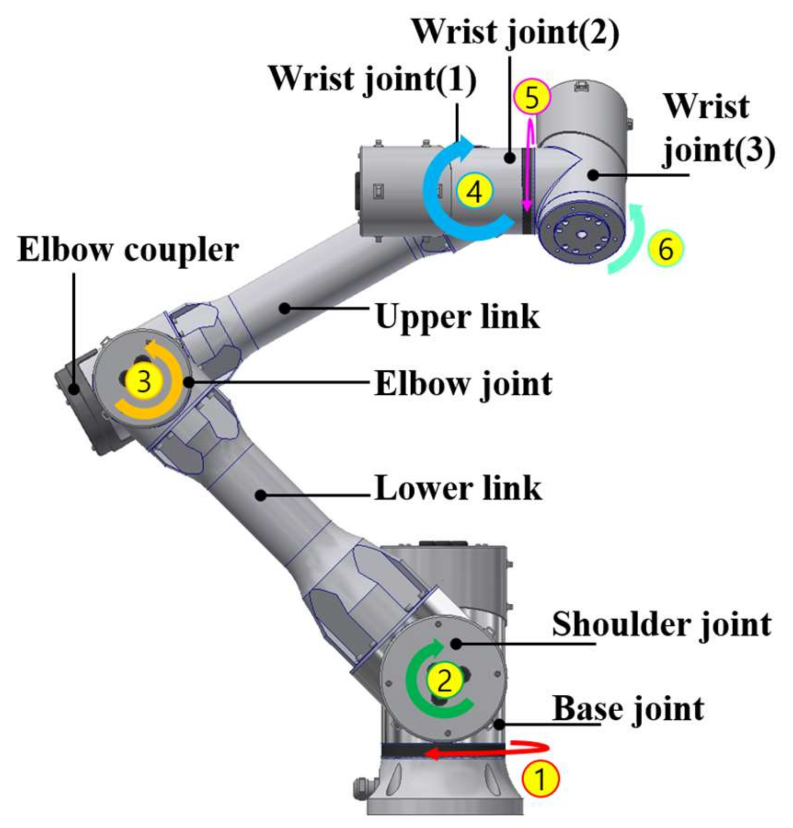
In this study, a six-degrees-of-freedom (6-DOF) articulated robot was considered to be the target robot as shown Figure 1. The designed joint motor and smart actuator were applied to this target robot. The robot has two links and six smart actuators, which act as the base, shoulder, elbow and three wrist joints.

Table 1. Robot Design Specifications.

Parameter	Unit	Value
Weight	kg	20
Payload	kg	5
Reach	mm	860
Joint ranges	deg	+/−360
Rated Joint Speed	deg/s	118.8
Rated Joint Acceleration	deg/s2	118.8
Degrees of freedom	-	6

summarizes the robot system specifications.

2.2. Joint Torque Calculation Method

The torque of each joint of the robot system was calculated through kinematics and dynamics analyses. First, the position, velocity, and acceleration profiles of each joint to the specified motion were generated through kinematic analysis. Then, based on the kinematic information, a rigid body dynamics analysis was performed to calculate the torque required for the smart actuator. For rigid body dynamics, the model is regarded a rigid body, and dynamic deformation is not considered. In general, to improve the position and control precision, the structure of an articulated robot hardly allows any structural deformation. In the structure of a robot, the most vulnerable part is the link connecting two joints. If the links in a robot system are sufficiently stiff, the system can be assumed a rigid body.

Therefore, we performed a stress analysis of the links of the robot, which are the most vulnerable to structural deformation. This analysis is described in this section. We show that the robot model can be assumed to be a rigid body. Then, modeling process of the robot system for kinematics and rigid body dynamics analyses too are explained.

2.2.1. Stress Analysis of Robot Links

As shown in Figure 1, the robot has two links. One is the lower link that connects the shoulder and elbow joints, and the other is the upper link that connects the elbow and wrist joints. The static deflection of the link was calculated by performing a three-dimensional finite element analysis (3D-FEA) for the actual link shape used in the robot to be developed. Static structural module of ANSYS Workbench software was used, and the general properties of aluminum 6061-T6 were applied as the material properties of the links.

As a constraint condition on stress analysis, one end of the link was fixed, and a static load was applied to the free end. The static load composed of the force and moment due to the weight of each component of robot, and payload [8,9]. The maximum static load that each link should support was calculated, and loads of 133.2 N and 48.75 Nm were applied to the lower link and 96.7 N and 10.95 to the upper link. Figure 2 shows how the mesh of the FEA model for each link and the calculated load conditions are applied to the FEA model.

Table 2. Results of Links Stress Analysis.

	Parameter	Unit	Value
Lower link	Deflection (δ) Equivalent stress (σ) Slope (δ/L)	mm MPa -	0.083 18.07 2.9 × 10−4
Upper link	Deflection (δ) Equivalent stress (σ) Slope (δ/L)	mm MPa -	0.045 8.30 1.7 × 10−4

lists the results of stress analysis. Figure 3 shows the contours of static deflection and Von-Mises equivalent stress for each link.

As an evaluation index of the static deflection $\left(\mathsf{\delta }\right)$ of the link, the deflection ratio $\left(\mathsf{\delta }/\mathrm{L}\right)$ for length $\left(\mathrm{L}\right)$ of each link was calculated. This ratio is the deflection slope. Since the deflection slope of the link converges to almost 0, it can be assumed that the model is a sufficiently rigid body. The stiffness of each link is also sufficient, as the analyzed maximum equivalent stress is significantly lower than the yield strength (276 MPa) of the link material aluminum 6061-T6.

2.2.2. Kinematics Analysis Model

When each joint is operated at the rated speed and rated acceleration, the motion that requires the maximum torque is analyzed first to estimate the maximum torque required for the joint. The joint torque was calculated from the moment of gravity force acting on the parts that move when the joint rotates and the driving acceleration of the joint [10].

The maximum torque is required when the center of gravity of the rotating body is the position at which the moment caused by gravity is the maximum, and the direction of driving acceleration is opposite to the moment caused by gravity. A free body diagram (FBD) of such a movement in the case of the shoulder joint is shown in Figure 4. Based on the FBD, the maximum torque required for the joint can be expressed using the moment equilibrium equation as shown in (1):

$$\begin{gathered} {\mathsf{\tau }}_j=I_o\times \alpha +M_g \\ {M}_g=F_g\times l=m_R\times g\times l \end{gathered}$$

(1)

where ${\mathsf{\tau }}_j$ is the torque of the joint; $I_o$ is the inertial moment for the center of rotation of the rotating body; $\alpha$ is the angular acceleration; $M_g$ is the moment of gravity force; $F_g$ is the gravity force; $l$ is the length from the center of rotation to the center of gravity; $m_R$ is the total mass of the rotating body; and $g$ is the gravitational acceleration.

Only three of the six actuators were selected for analysis. Joints were selected based on the consideration that whether or not the gravity acting on the rotating body supported by each joint acts as the load moment of the joint. The joints that satisfy this requirement can be any joint depending on the posture of the robot. However, in the case of the wrist joints, the wrist (1) subjected to the maximum load moment to support the wrist (2), wrist (3), payload all. Therefore, from among wrist joints, we considered only wrist (1) that requires the most torque.

To calculate the maximum torque for the three selected joints, we considered the motion shown in Figure 5.

The position where all the joints of the robot were placed perpendicular to the ground was set as the initial position ($0°$), and the planar motion was set such that the joints to be analyzed repeatedly moved in the $-90°$ and $90°$ sections.

2.2.3. Rigid Body Dynamics Analysis Model

A rigid body dynamics analysis was performed using Altair-Inspire software. The solver solves a generalized equation of motion in the form of differential algebraic equations such as (2) for multibody systems using the state-space method for given input variables [11]:

$$M\ddot{q}+{\Phi }_q^T=f\left(q,\dot{q}\right)$$

(2)

where $M$ is the mass inertia matrix of the system; $q,\dot{q},\ddot{q}$ are the displacement, velocity, and acceleration vectors, respectively, for the generalized coordinates of the system; ${\Phi }_q^T$ is the Jacobian matrix for the kinematic constraints; $\lambda$ is a Lagrange multiplier vector representing the kinematic constraint force; and $f\left(q,\dot{q}\right)$ is the generalized force vector.

To define the rigid body dynamics analysis model of the robot system to be developed, we considered a previous version of the robot system with similar specifications, i.e., the mass of each part was assumed to be in proportion to the mass of the robot parts of the previous version based on the expected dimensions and target total weight. The center of gravity was calculated based on the expected positions of the stator core of the joint motor and the reducer, which have relatively large weight among the components of the smart actuator. The moment of inertia of the smart actuator and the link was calculated by considering the shape of the parts as a solid or hollow cylinder. The kinematic constraints are the revolute joints defined for each joint. Figure 6 shows the shape of the simplified 3D analysis model and the mass table calculated for each part.

2.2.4. Kinematics Analysis Result

Figure 7 shows the results of the kinematic analysis of the shoulder, elbow, and wrist (1) joints selected for analysis. It shows the speed and position profiles of each joint when driving the trajectory of planar motion at the rated speed and the rated acceleration. This profile is the same for all joints because the operating conditions of each joint are the same.

2.2.5. Rigid Body Dynamics Analysis Result

A rigid body dynamics analysis was performed using the speed profile shown in Figure 7 as the input conditions for the shoulder, elbow, and wrist joints.

Figure 8 and Figure 9 show the torque and power, respectively, required for each joint as by the analysis.

Table 3. Calculated Torque and Power for Smart Actuators in Each Joint.

Joint	Parameter	Unit	Value
Shoulder	Torque	N∙m	111.5
	Power	W	151.4
Elbow	Torque	N∙m	45.8
	Power	W	61.2
Wrist(1)	Torque	N∙m	6.7
	Power	W	8.8

lists the maximum required torque and power of the smart actuator derived by rigid body dynamics analysis. However, these are ideal specifications. This is because these specifications do not reflect the effects of lubrication and the viscosity and Coulomb friction effects caused by the contact between the mechanical parts or between the gear teeth of the reducer. Therefore, when determining the specifications of the joint motor, it is necessary to introduce a margin considering the friction effect and reducer loss.

3. Design of the Joint Motor

3.1. Joint Motor Design Specifications

The main design requirements of the joint motor used in the joint robot with the 5-kg payload are listed in

Table 4. Design Requirements of Joint Motors.

Items	Unit	Wrist Joint Motors	Elbow Joint Motor	Base-Shoulder Joint Motors
		Type-I	Type-II	Type-III
Rated Power	W	60	120	300
Rated Torque	Nm	0.29	0.58	1.44
Rated Speed	rpm	2000
Outer Diameter	mm	58	58	75.5
Input Voltage	V	48
Cooling Type	-	Natural Cooling
Temperature Constraint	°C	100 (Winding)
Magnet Material		Nd-Fe-B
Core Material		35PN440

. Based on the torque and power calculated by the rigid body dynamics analysis, we determined the power requirement specifications of the joint motor considering the mechanical losses, margin, and the efficiency of the reducer. The joint motors to be used for the smart actuators of the wrist, elbow, and shoulder joints were defined as Type-I, Type-II, and Type-III, respectively.

Considering the limited space of the smart actuator, the outer diameter for each joint motor was fixed. The motor axial length should be minimized to obtain the smallest possible system. Moreover, the temperature of the winding should be less than 100 °C to ensure the safety and reliability of the joint motor. These dimensions and temperature conditions were considered to be the design constraints.

3.2. Electromagnetic Design

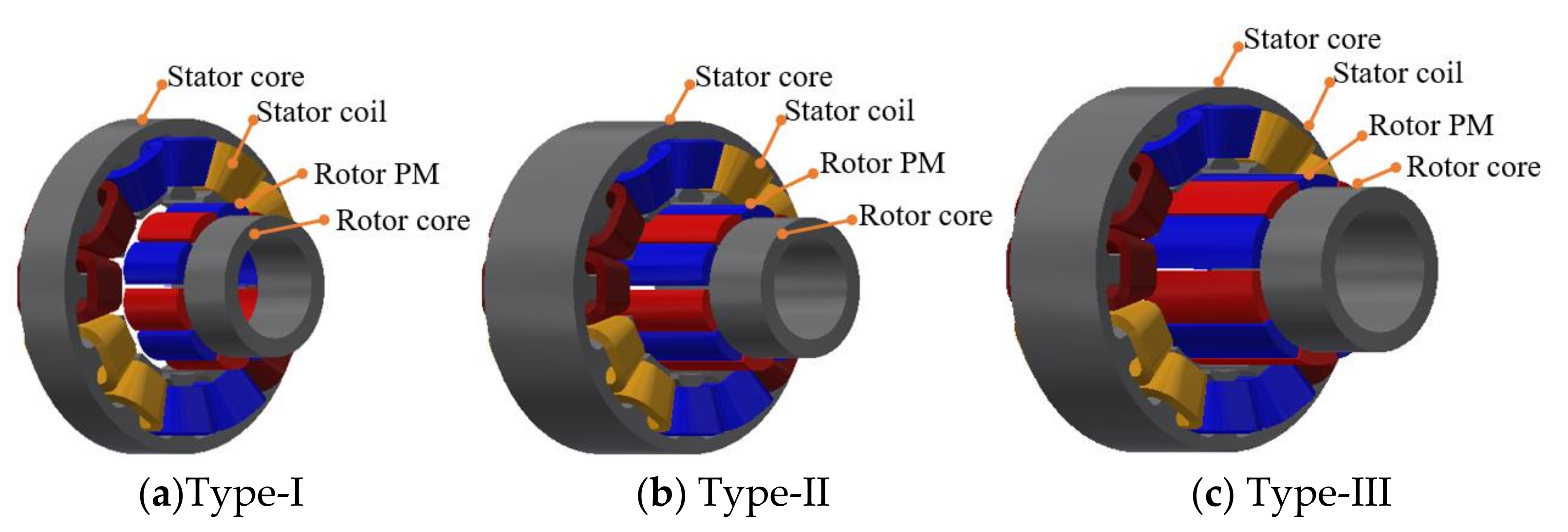
Figure 10 shows the overall design process for the joint motors. In the preliminary design step, the stacking length, air-gap length, and fill factor were determined considering the design requirements and constraints. Several slot and pole combinations were compared considering the electromagnetic and mechanical characteristics to choose the best-suited model for this robot application. To ensure a fair comparison of these slot and pole combination models, we used identical conditions such as the rotor and stator inner/outer diameters, motor axial length, and magnet volume for all models.

The winding specifications were designed specifically to obtain the required torque and satisfy the voltage constraints. We selected with 10-pole-12-slot specifications with a high winding factor, high cogging torque frequency, and high torque constant.

To reduce the cogging torque of motors further, we chose the magnet arc and slot opening as the design variables in the optimum design step using the response surface methodology combined with two-dimensional finite element analysis (2D-FEA) [12,13,14]. However, the output torque also decreased accordingly. To compensate for the reduced torque and to operate the Hall IC sensor, we used the magnet overhang.

The electromagnetic characteristics of the designed motors were analyzed through 2D-FEA using Maxwell software tool. The overhang effect was considered in the 2D simulation by compensating the permanent magnetic flux density of magnetic materials using the overhang ratio [15,16,17]. The configurations of the final models are shown in Figure 11. As given in

Table 5. Performance of the Designed Joint Motors.

Items	Unit	Type-I	Type-II	Type-III
Rated Output Power	W	60	120	300
Stator Axial Length	mm	11	22	25
Rotor Axial Length	mm	13	26	32
Back-EMF at 2000 rpm	Vline-rms	18.4	19.7	20.6
Torque Density	Nm/kg	1.6	1.8	2.3
Cogging Torque	%	0.49	0.46	0.14
Efficiency	%	85.1	88.2	91.4

, the cogging torque of all models is less than 1% of the rated torque, and the back-electromotive force (back-EMF) value is smaller than the input voltage within the maximum operating speed range. Therefore, the electromagnetic design requirements are met.

3.3. Thermal Analysis

The copper and iron losses as seen from the 2D-FEA for each type are listed in

Table 6. Loss Data of the Designed Joint Motors.

Items	Unit	Type-I	Type-II	Type-III
Input Current	A-rms	2.0	3.8	8.5
Resistance	Ω	0.8	0.4	0.1
Core Loss	W	1.0	2.0	4.7
Copper Loss	W	10.0	15.1	22.9

. The eddy current loss in the magnet is sufficiently small to be neglected in this study. These losses were considered to be heat sources in the thermal analysis using the lump-parameter-thermal-network method. The thermal network was constructed using the thermal resistances and power sources.

The thermal problem was solved by calculating a set of nonlinear equations at each node:

$$C\frac{dT}{dt}+\frac{T}{R}=P$$

(3)

where $C=\rho V{C}_P$ is the heat capacitance; $T$ is the temperature rise; $P$ is the power source; $R$ is the thermal resistance; $\rho$ is the density; $V$ is the volume of the component; and $C_P$ is the specific heat capacity of the material [18].

The thermal resistances were determined by considering the conduction, convection, and radiation heat transfer mechanisms. The heat transfer in the air gap was considered to be forced convection due to the rotor rotation and that between the housing and the surrounding air is considered to be natural convection. The calculation method of these convection coefficients was presented in detail in [19,20]. The reliability of the thermal analysis depends on not only the accuracy of the convection coefficient, but also the material properties. The thermal properties of the main materials used in this study are listed in

Table 7. Material Properties for Thermal Analysis.

Motor Part	Thermal Conductivity (W/m/°C)	Specific Heat (J/kg/°C)	Density (kg/m3)
Rotor and stator core	30	460	7600
Winding	401	385	8933
Magnet	7.6	460	7500
Housing	96	880	2800

.

By applying the loss calculated from FEA as heat sources and heat transfer coefficients for resistance calculation, we derived the estimated winding temperatures by solving the thermal network [21,22,23,24]. The detailed thermal equivalent circuit of the motor has been presented in [18].

Table 8. Analysis and test results of Winding temperature and Back-EMF line voltage.

Items	Unit	Type-I	Type-II	Type-III
Analysis Winding Temperature	℃	74.8	88.9	83.0
Test Winding Temperature	℃	62.2	89.1	88.9
Analysis Back-EMF @ 2000 rpm	Vline-rms	18.4	19.7	20.6
Test Back-EMF @ 2000 rpm	Vline-rms	17.5	18.6	20

lists the thermal analysis and test results of the joint motors, along with the back-EMF analysis and test results. The thermal test results and back-EMF results will be discussed in Section 4. The thermal analysis proves that all three designed motors satisfied the temperature constraint with maximum winding temperatures less than 100 °C.

4. Motor Performance Test

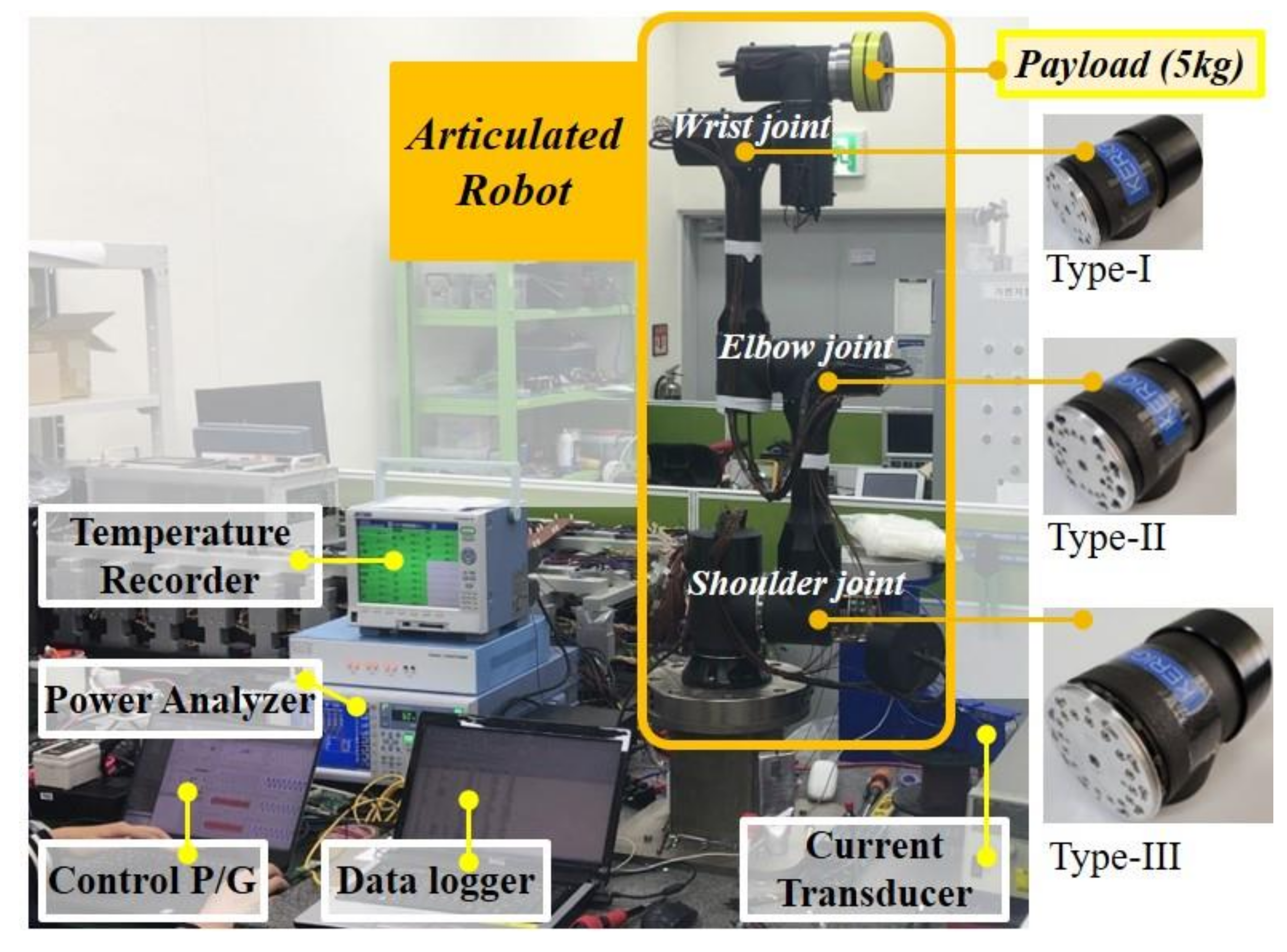
Three prototypes of joint motors were manufactured and tested based on the design specifications. The prototypes are shown in Figure 12.

Three types of performance tests were conducted, each with a different purpose. The first test was performed to check the manufacturing status of the prototypes by measuring the back-EMF and the mechanical loss under the no-load condition. The second was performed to confirm the output performance of the prototypes through a load fluctuation test according to the speed. Finally, the prototypes were continuously driven at the rated output state to measure the saturation temperature of the winding, and the thermal stability was confirmed by comparative analysis with the thermal analysis results.

4.1. No-Load Condition Test

Figure 13 shows the back-EMF and mechanical loss according to the speed as measured through the no-load test. The back-EMF increases linearly with speed, and there is no significant difference between the measured values of the prototypes and the analysis values of the design models (see Table 8). Therefore, all prototypes were regarded as designed and built within a range that does not significantly affect the output performance. The mechanical loss increased nonlinearly with speed, and at the rated speed, the mechanical loss accounted for about 4–7% of the rated power. This value was not considered a loss or heat source in the motor design process. This added value serves to reduce efficiency and increase the temperature.

4.2. Test under Loads

The input and output characteristics of each prototype were measured with variations in speed and load. The speed was measured up to 3000 rpm, and the load was measured up to the rated torque of each prototype. Figure 14 shows the input current map to obtain the load torque according to speed. The input current map shows that the relationship between the torque and current remains almost linear at all test points, including the operating points above the rated conditions.

4.3. Temperature Saturation Test

The temperature saturation test was conducted under continuous rated operating conditions until the temperature change of the coil was less than 1° for 30 min.

Figure 15 shows that all saturation temperatures are thermally stable because they are below the temperature limit of 100 °C, which was predicted in the thermal analysis (see Table 8). Table 8 compares the average value of the temperature distribution of the coil in the thermal analysis and the measured value at any point of the coil ad it shows that the analysis results are relatively correct.

Since the temperature distribution in the coil was non uniform even during saturation, all three models are regarded to have predicted the temperature well.

5. Articulated Robot System Performance Test

To apply the manufactured joint motor to an articulated robot system and test its performance, three types of smart actuators classified by capacity were manufactured. The smart actuator was manufactured by assembling a harmonic drive with a reduction ratio of 1:101 to a joint motor. Then, the manufactured smart actuators were assembled with the links to complete a 6-DOF articulated robot. Figure 16 shows a performance test system for a smart actuator as applied to an articulated robot system. A maximum payload of 5 kg was applied for comparative analysis with the results of the rigid body dynamics analysis. In addition, the motion, operating speed, and acceleration of each joint were set in the same manner as for the rigid body dynamics analysis. The tests were performed on the shoulder, elbow, and wrist (1) joints.

5.1. Joint Motor Torque Estimation

The manufactured smart actuator did not have a built-in sensor to measure torque and force. Therefore, the input current and the operating speed were measured, and the torque of the joint motor was estimated according to the relationship between the input current, the speed, and the torque, as shown in Figure 14. The torque of the smart actuator was estimated using the relational expression between the torque of the joint motor and the reduction ratio of the harmonic drive [25]. Figure 17 shows the phase input current and speed profiles as measured by the joint motors inside each smart actuator. To estimate the maximum torque of each joint motor, the torque value was obtained by associating the current at the maximum input current and the speed value at that time with reference to Figure 14.

With reference to panels (a) in Figure 17, the point where the input current of the joint motor is the maximum is near point $C$ when the robot starts accelerating in the direction opposite to that of the gravitational moment while being horizontal to the ground. Ideally, the input current at point $C$ should be the maximum, but in reality, a time delay is caused by the rise time until the required input current is reached. Therefore, the input current reached the maximum value at point $C^{\prime }$ a little later than at point $C$, and the maximum torque was estimated based on the input current and speed values at point $C^{\prime }$ for each joint motor.

Table 9. Estimated Torque of Joint Motors.

Joint	Parameter	Unit	Value
Shoulder (Type-III)	Input current	A-rms	11.63
	Speed	RPM	500
	Estimated torque	N∙m	1.55
Elbow (Type-II)	Input current	A-rms	4.82
	Speed	RPM	516
	Estimated torque	N∙m	0.7
Wrist (1) (Type-I)	Input current	A-rms	1.117
	Speed	RPM	1280
	Estimated torque	N∙m	0.179

lists the estimated maximum torque analysis results of the joint motors.

5.2. Smart Actuator Torque Estimation

To compare the test results with the results of rigid body dynamics analysis, the actual maximum torque of the smart actuator was estimated using the estimated maximum torque of the joint motor and using a relational expression such as that shown in (4).

$${\tau }_{act}={\tau }_m\times i_g\times {\eta }_g$$

(4)

where ${\tau }_{act}$ is the estimated torque of the smart actuator; ${\tau }_m$ is the estimated motor torque; $i_g$ is the reduction ratio of the harmonic drive; and ${\eta }_g$ is the efficiency of the harmonic drive. The reduction ratios of the harmonic drives used for each smart actuator were all 1:101, and the efficiency of the harmonic drives was the numerical value described in the data sheet provided by the manufacturer Nidec Co. Ltd., Japan.

A comparison of the experimentally estimated value and the analytically derived value for the maximum torque of each smart actuator showed that both values were approximately close for all joints as shown in Figure 18.

6. Conclusions

In this paper, we described the process of efficiently designing joint motors, which are the driving components of an articulated robot, for cooperative robots. The joint motors designed by the proposed design method were manufactured, and their performance were tested not only at the component level, but also at the system level to examine the usefulness of the proposed design method.

In conclusion, the analysis value and the experimentally estimated value for the output torque set as the standard of the output specification in the design process were similar. The shoulder joint to which the Type-III joint motor was applied and the elbow joint to which the Type-II joint motor was applied showed an error rate within 10%. In the case of the wrist joint(1) to which Type-I is applied, the required torque is numerically low. Therefore, although the numerical difference was small, the error rate was large compared to the other two joints.

The causes of the error may be mechanical friction and lubrication loss ignored according to the rigid body dynamics analysis theory, the difference in mass and inertia parameters between the analysis model and the manufacturing model, and the control error of the joint motor. Even if there is a cause of these errors, the level of the error is small, so the rigid body dynamics analysis method was sufficiently effective as a method for determining the basic specifications of the joint motor.

In addition, a margin was set in consideration of the efficiency of the reducer based on the derived basic specifications. The suitability of the margin was confirmed by performing multi-physical analysis. The reliability of the analysis was also verified by comparing the analysis values with the experimental values for the output characteristics and thermal performance of the joint motor.

Through this process, the usefulness of the proposed joint motor design process has been verified, and the series of processes provided in this article will be helpful for determining the appropriate specifications of the joint motors for the robot system.

References

- Wang, Y.; Li, K.; Zhou, H.; Deng, S.; Xu, J.; Liu, J. Dynamic Analysis and Co-Simulation ADAMS-SIMULINK for a Space Manipulator Joint. In Proceedings of the 2015 International Conference on Fluid Power and Mechatronics (FPM), Harbin, China, 5–7 August 2015; pp. 984–989. [Google Scholar]
- Yin, H.; Yu, Y.; Li, J. Optimization Design of a Motor Embedded in a Lightweight Robotic Joint. In Proceedings of the 2017 12th IEEE Conference on Industrial Electronics and Applications (ICIEA), Siem Reap, Cambodia, 18–20 June 2017; pp. 1630–1634. [Google Scholar]
- Seo, J.; Rhyu, S.; Kim, J.; Choi, J.; Jung, I. Design of Axial Flux Permanent Magnet Brushless DC Motor for Robot Joint Module. In Proceedings of the The 2010 International Power Electronics Conference-ECCE ASIA, Sapporo, Japan, 21–24 June 2010; pp. 1336–1340. [Google Scholar]
- Srinivas, G.L.; Javed, A. Topology Optimization of KUKA KR16 Industrial Robot Using Equivalent Static Load Method. In Proceedings of the 2021 IEEE International IOT, Electronics and Mechatronics Conference (IEMTRONICS), Toronto, ON, Canada, 21 April 2021; pp. 1–6. [Google Scholar]
- Lee, K.; Lee, J.; Woo, B.; Lee, J.; Lee, Y.; Ra, S. Modeling and Control of a Articulated Robot Arm with Embedded Joint Actuators. In Proceedings of the 2018 International Conference on Information and Communication Technology Robotics (ICT-ROBOT), Busan, Korea, 6−8 September 2018; pp. 1–4. [Google Scholar]
- Choi, W.-J.; Yoon, M.-K.; Bang, Y.-B.; Cho, H.-S. Design and Fabrication of High-Power Smart Actuator Module. In Proceedings of the 2011 IEEE/SICE International Symposium on System Integration (SII), Koyto, Japan, 20–22 December 2011; pp. 434–439. [Google Scholar]
- Park, C.; Kyung, J.H.; Choi, T. Design of a Human-Robot Cooperative Robot Manipulator Using SMART Actuators. In Proceedings of the 2011 11th International Conference on Control, Automation and Systems, Hokkaido, Japan, 6–9 October 2011; pp. 1868–1870. [Google Scholar]
- Yao; Zhou; Lin; Tang Light-Weight Topological Optimization for Upper Arm of an Industrial Welding Robot. Metals 2019, 9, 1020. [CrossRef] [Green Version]
- Bugday, M.; Karali, M. Design Optimization of Industrial Robot Arm to Minimize Redundant Weight. Eng. Sci. Technol. Int. J. 2019, 22, 346–352. [Google Scholar] [CrossRef]
- Tang, J.; Cheng, L.; Liu, J.; Wang, Y.; Liu, R. An Integrated Joint for Cooperative Robots. In Proceedings of the 2019 IEEE International Conference on Advanced Robotics and its Social Impacts (ARSO), Beijing, China, 31 October–2 November 2019; pp. 97–101. [Google Scholar]
- Parameters: Transient Solver. Available online: https://2020.help.altair.com/2020.1/hwsolvers/ms/topics/solvers/ms/xml-format_79.htm (accessed on 5 October 2021).
- He, C.; Wu, T. Analysis and Design of Surface Permanent Magnet Synchronous Motor and Generator. Trans. Electr. Mach. Syst. 2019, 3, 94–100. [Google Scholar] [CrossRef]
- Kim, H.-J.; Kim, D.-Y.; Hong, J.-P. Structure of Concentrated-Flux-Type Interior Permanent-Magnet Synchronous Motors Using Ferrite Permanent Magnets. IEEE Trans. Magn. 2014, 50, 1–4. [Google Scholar] [CrossRef]
- Lee, S.G.; Kim, K.-S.; Lee, J.; Kim, W.H. A Novel Methodology for the Demagnetization Analysis of Surface Permanent Magnet Synchronous Motors. IEEE Trans. Magn. 2016, 52, 1–4. [Google Scholar] [CrossRef]
- Kim, K.; Koo, D.; Lee, J. The Study on the Overhang Coefficient for Permanent Magnet Machine by Experimental Design Method. IEEE Trans. Magn. 2007, 43, 2483–2485. [Google Scholar] [CrossRef]
- Yeo, H.; Park, H.; Seo, J.; Jung, S.; Ro, J.; Jung, H. Electromagnetic and Thermal Analysis of a Surface-Mounted Permanent-Magnet Motor with Overhang Structure. IEEE Trans. Magn. 2017, 53, 1–4. [Google Scholar] [CrossRef]
- Song, J.; Lee, J.H.; Kim, Y.; Jung, S. Computational Method of Effective Remanence Flux Density to Consider PM Overhang Effect for Spoke-Type PM Motor With 2-D Analysis Using Magnetic Energy. IEEE Trans. Magn. 2016, 52, 1–4. [Google Scholar] [CrossRef]
- Zhao, N.; Liu, W. Loss Calculation and Thermal Analysis of Surface-Mounted PM Motor and Interior PM Motor. IEEE Trans. Magn. 2015, 51, 1–4. [Google Scholar] [CrossRef]
- Luu, P.T.; Lee, J.; Lee, J.; Park, J. Electromagnetic and Thermal Analysis of Permanent-Magnet Synchronous Motors for Cooperative Robot Applications. IEEE Trans. Magn. 2020, 56, 1–4. [Google Scholar] [CrossRef]
- Luu, P.T.; Lee, J.-Y.; Lee, J.-H.; Park, J.-W. Electromagnetic and Thermal Analysis of a Permanent Magnet Motor Considering the Effect of Articulated Robot Link. Energies 2020, 13, 3239. [Google Scholar] [CrossRef]
- Boglietti, A.; Cavagnino, A.; Staton, D.; Shanel, M.; Mueller, M.; Mejuto, C. Evolution and Modern Approaches for Thermal Analysis of Electrical Machines. IEEE Trans. Ind. Electron. 2009, 56, 871–882. [Google Scholar] [CrossRef] [Green Version]
- Qi, J.; Hua, W.; Zhang, H. Thermal Analysis of Modular-Spoke-Type Permanent-Magnet Machines Based on Thermal Network and FEA Method. IEEE Trans. Magn. 2019, 55, 1–5. [Google Scholar] [CrossRef]
- Yunkai Huang; Jianguo Zhu; Youguang Guo Thermal Analysis of High-Speed SMC Motor Based on Thermal Network and 3-D FEA With Rotational Core Loss Included. IEEE Trans. Magn. 2009, 45, 4680–4683. [CrossRef]
- Zhu, Z.; Zhang, W.; Li, Y.; Guo, J. Thermal Analysis of Axial Permanent Magnet Flywheel Machine Based on Equivalent Thermal Network Method. IEEE Access 2021, 9, 33181–33188. [Google Scholar] [CrossRef]
- Song, J.; Xu, F.; Zou, F.; Chen, S.; Zhao, B. Joint Torque Detection Based on Motor Current and Singular Perturbation Control for Cleaning Room Manipulator. In Proceedings of the 2017 IEEE 7th Annual International Conference on CYBER Technology in Automation, Control, and Intelligent Systems (CYBER), Honolulu, HI, USA, 31 July–4 August 2017; pp. 1609–1614. [Google Scholar]
Figure 1.
Conceptual diagram of joints and links of the target articulated robot.
Figure 2.
Meshes and load conditions for the FEA model of each link: (a) Upper link mesh; (b) upper link load conditions; (c) lower link mesh; and (d) lower link load conditions.
Figure 3.
Link stress analysis results: (a) Upper link deflection; (b) upper link equivalent stress; (c) lower link deflection; and (d) lower link equivalent stress.
Figure 4.
Free body diagram for situations where maximum torque is required for a joint.
Figure 5.
Motion schematic to analyze the maximum torque of each joint.
Figure 6.
Simplified 3D analytical model of robot.
Figure 7.
Speed and position profiles of the joint according to the set planar motion trajectory.
Figure 8.
Required torque for each joint.
Figure 9.
Required power for each joint.
Figure 10.
Joint motor design process.
Figure 11.
3D configuration of final model for each joint motor.
Figure 12.
Three types of joint motors and smart actuators.
Figure 13.
No-load test results: (a) Back-EMF, (b) Mechanical loss.
Figure 14.
Load test result: input current map for three types: (a) Type-I; (b) Type-II; and (c) Type-III.
Figure 15.
Thermal performance test result: Motor winding temperature.
Figure 16.
Performance test system for smart actuators applied to the robot.
Figure 17.
Input current and speed profile measured at the joint motor within each smart actuator: (a) Shoulder joint; (b) Elbow joint; and (c) Wrist joint(1).
Figure 18.
Comparison of the estimated and analytical values of the maximum torque for each smart actuator.